Identifying the Distribution of Treatment Effects
under Support Restrictions

Abstract

The distribution of treatment effects (DTE) is often of interest in the context of welfare policy evaluation. In this paper, I consider partial identification of the DTE under known marginal distributions and support restrictions on the potential outcomes. Examples of such support restrictions include monotone treatment response, concave treatment response, convex treatment response, and the Roy model of self-selection. To establish informative bounds on the DTE, I formulate the problem as an optimal transportation linear program and develop a new dual representation to characterize the identification region with respect to the known marginal distributions. I use this result to derive informative bounds for concrete economic examples. I also propose an estimation procedure and illustrate the usefulness of my approach in the context of an empirical analysis of the effects of smoking on infant birth weight. The empirical results show that monotone treatment response has a substantial identifying power for the DTE when the marginal distributions of the potential outcomes are given.

1 Introduction

In this paper, I study partial identification of the distribution of treatment effects (DTE) under a broad class of restrictions on potential outcomes. The DTE is defined as follows: for any fixed $\delta\in$ $\mathbb{R},$

$$F_{\Delta}\left(\delta\right)=\Pr\left(\Delta\leq\delta\right),$$

with the treatment effect $\Delta=Y_{1}-Y_{0}$ where $Y_{0}$ and $Y_{1}$ denote the potential outcomes without and with some treatment, respectively. The question that I am interested in is how treatment effects or program benefits are distributed across the population.

In the context of welfare policy evaluation, distributional aspects of the effects are often of interest, e.g. ”which individuals are severely affected by the program?” or ”how are those benefits distributed across the population?”. As Heckman et al. (1997) pointed out, the DTE is particularly important when treatments produce nontransferable and nonredistributable benefits such as outcomes in health interventions, academic achievement in educational programs, and occupational skills in job training programs or when some individuals experience severe welfare changes at the tails of the impact distribution.

Although most empirical research on program evaluation has focused on average treatment effects (ATE) or marginal distributions of potential outcomes, these parameters are limited in their ability to capture heterogeneity of the treatment effects at the individual level. For example, consider two projects with the same average benefits, one of which concentrates benefits among a small group of people, while the other distributes benefits evenly across the population. ATE cannot differentiate between the two projects because it shows only the central tendency of treatment effects as a location parameter, whereas the DTE captures information about the entire distribution. Marginal distributions of $Y_{0}$ and $Y_{1}$ are also uninformative about parameters on the individual specific heterogeneity in treatment effects including the fraction of the population that benefits from a program $\Pr\left(Y_{1}\geq Y_{0}\right),$ the fraction of the population that has gains or losses in a specific range $\Pr\left(\delta^{L}\leq Y_{1}-Y_{0}\leq\delta^{U}\right)$, the $q$-quantile of the impact distribution $\inf\left\{\delta:F_{\Delta}\left(\delta\right)>q\right\}$, etc. See, e.g. Heckman et al. (1997), Abbring and Heckman (2007), and Firpo and Ridder (2008), among others for more details.

Despite the importance of these parameters in economics, related empirical research has been hampered by difficulties associated with identifying the entire distribution of effects. The central challenge arises from a missing data problem: under mutually exclusive treatment participation, econometricians can observe either a treated outcome or an untreated outcome, but both potential outcomes $Y_{0}$ and $Y_{1}$ are never simultaneously observed for each agent. Therefore, the joint distribution of $Y_{0}$ and $Y_{1}$ is not typically exactly identified, which complicates identification of the DTE, which is point-identified only under strong assumptions about each individual’s rank across the treatment status or specifications on the joint distribution of $Y_{0}$ and $Y_{1}$, which are often not justified by economic theory or plausible priors.

This paper relies on partial identification to avoid strong assumptions and remain cautious of assumption-driven conclusions. In the related literature, Manski (1997) established bounds on the DTE under monotone treatment response (MTR), which assumes that the treatment effects are nonnegative. Fan and Park (2009, 2010) and Fan and Wu (2010) adopted results from copula theory to establish bounds on the DTE, given marginal distributions. Unfortunately, both approaches deliver bounds that are often too wide to be informative in practice. Since these two conditions are often plausible in practice, a natural way to tighten the bounds is considering both MTR and given marginal distributions of potential outcomes. However, methods of establishing informative bounds on the DTE under these two restrictions have remained unanswered. Specifically, in the existing copula approach it is technically challenging to find out the particular joint distributions that achieve the best possible bounds on the DTE under the two restrictions.

In this paper, I propose a novel approach to circumvent these difficulties associated with identifying the DTE under these two restrictions. Methodologically, my approach involves formulating the problem as an optimal transportation linear program and embedding support restrictions on the potential outcomes including MTR into the cost function. A key feature of the optimal transportation approach is that it admits a dual formulation. This makes it possible to derive the best possible bounds from the optimization problem with respect to given marginal distributions but not the joint distribution, which is an advantage over the copula approach. Specifically, the linearity of support restrictions in the entire joint distribution allows for the penalty formulation. Since support restrictions hold with probability one, the corresponding multiplier on those constraints should be infinite. To the best of my knowledge, the dual representation of such an optimization problem with an infinite Lagrange multiplier has not been derived in the literature. In this paper, I develop a dual representation for $\{0,1,\infty\}$-valued costs by extending the existing result on duality for $\{0,1\}$-valued costs.

My approach applies to general support restrictions on the potential outcomes as well as MTR. Such support restrictions encompass shape restrictions on the treatment response function that can be written as $g\left(Y_{0},Y_{1}\right)\leq 0$ with probability one for any continuous function $g:\mathbb{R}\rightarrow\mathbb{R}$, including MTR, concave treatment response, and convex treatment response. Moreover, considering support restrictions opens the way to identify the DTE in the Roy model of self-selection and the DTE conditional on some sets of potential outcomes.

Numerous examples in applied economics fit into this setting because marginal distributions are point or partially identified under weak conditions and support restrictions are often implied by economic theory and plausible priors. The marginal distributions of the potential outcomes are point-identified in randomized experiments or under unconfoundedness. Even if selection depends on unobservables, they are point-identified for compliers under the local average treatment effects assumptions (Imbens and Rubin (1997), Abadie (2002)) and are partially identified in the presence of instrumental variables (Kitagawa (2009)). Also, MTR has been defended as a plausible restriction in empirical studies of returns to education (Manski and Pepper (2000)), the effect of funds for low-ability pupils (Haan (2012)), the impact of the National School Lunch Program on children’s health (Gundersen et al. (2011)), and various medical treatments (Bhattacharya et al. (2005, 2012)). Researchers sometimes have plausible information on the shape of treatment response functions from economic theory or from empirical results in previous studies. For example, based on diminishing marginal returns to production, one may find it plausible to assume that the marginal effect of improved maize seed adoption on productivity diminishes as the level of adoption increases, holding other inputs fixed. Also, one may want to assume that the marginal adverse effect of an additional cigarette on infant birth weight diminishes as the number of cigarettes increases as shown in Hoderlein and Sasaki (2013). In the empirical literature, concave treatment response has been assumed for returns to schooling (Okumura (2010)) and convex treatment response for the effect of education on smoking (Boes (2010)).

A considerable amount of the literature has used the Roy model to describe people’s self-selection ranging from immigration to the U.S. (Borjas (1987)) to college entrance (Heckman et al. (2011)). Also, heterogeneity in treatment effects for unobservable subgroups defined by particular sets of potential outcomes has been of central interest in various empirical studies. Heterogeneous peer effects and tracking impacts (Duflo et al. (2011)) and heterogeneous class size effects (Ding and Lehrer (2008)) by the level of students’ performance, and the heterogeneity in smoking effects by potential infant’s birth weight (Hoderlein and Sasaki (2013)) have also been discussed in the literature focusing on heterogeneous average effects.

I apply my method to an empirical analysis of the effects of smoking on infant birth weight. I propose an estimation procedure and illustrate the usefulness of my approach by showing that MTR has a substantial identifying power for the distribution of smoking effects given marginal distributions. As a support restriction, I assume that smoking has nonpositive effects on infant birth weight. Smoking not only has a direct impact on infant birth weight, but is also associated with unobservable factors that affect infant birth weight. To overcome the endogenous selection problem, I make use of the tax increase in Massachusetts in January 1993 as a source of exogenous variation. I point-identify marginal distributions of potential infant birth weight with and without smoking for compliers, which indicate pregnant women who changed their smoking status from smoking to nonsmoking in response to this tax shock. To estimate the marginal distributions of potential infant birth weight, I use the instrumental variables (IV) method presented in Abadie et al. (2002). Furthermore, I estimate the DTE bounds using plug-in estimators based on the estimates of marginal distribution functions. As a by-product, I find that the average adverse effect of smoking is more severe for women with a higher tendency to smoke and that smoking women with some college and college graduates are less likely to give births to low birth weight infants than other smoking women.

In the next section, I give a formal description of the basic setup, notation, terms and assumptions throughout this paper and present concrete examples of support restrictions. I review the existing method of identifying the DTE given marginal distributions without support restrictions to demonstrate its limits in the presence of support restrictions. I also briefly discuss the optimal transportation approach to describe the key idea of my identification strategy. Section 3 formally characterizes the identification region of the DTE under general support restrictions and derives informative bounds for economic examples from the characterization. Section 4 provides numerical examples to assess the informativeness of my new bounds and analyzes sources of identification gains. Section 5 illustrates the usefulness of these bounds by applying DTE bounds derived in Section 3 to an empirical analysis of the impact distribution of smoking on infant birth weight. Section 6 concludes and discusses interesting extensions.

2 Basic Setup, DTE Bounds and Optimal Transportation Approach

In this section, I present the potential outcomes setup that this study is based on, the notation, and the assumptions used throughout this study. I demonstrate that the bounds on the DTE established without support restrictions are not the best possible bounds in the presence of support restrictions. Then I propose a new method to derive sharp bounds on the DTE based on the optimal transportation framework.

2.1 Basic Setup

The setup that I consider is as follows: the econometrician observes a realized outcome variable $Y$ and a treatment participation indicator $D$ for each individual, where $D=1$ indicates treatment participation while $D=0$ nonparticipation. An observed outcome $Y$ can be written as $Y=DY_{1}+(1-D)Y_{0}$. Only $Y_{1}$ is observed for the individual who takes the treatment while only $Y_{0}$ is observed for the individual who does not take the treatment, where $Y_{0}$ and$\ Y_{1}$ are the potential outcome without and with treatment, respectively. Treatment effects $\Delta$ are defined as $\Delta=Y_{1}-Y_{0}$ the difference of potential outcomes. The objective of this study is to identify the distribution function of treatment effects $F_{\Delta}\left(\delta\right)=\Pr\left(Y_{1}-Y_{0}\leq\delta\right)$ from observed pairs $\left(Y,D\right)$ for fixed $\delta\in\mathbb{R}$ .

To avoid notational confusion, I differentiate between the distribution and the distribution function. Let $\mu_{0}$, $\mu_{1}$ and $\pi$ denote marginal distributions of $Y_{0}$ and $Y_{1}$, and their joint distribution, respectively. That is, for any measurable set $A_{d}$ in $\mathbb{R}$, $\mu_{d}\left(A_{d}\right)=\Pr\left\{Y_{d}\in A_{d}\right\}$ for $d\in\left\{0,1\right\}$ and $\pi\left(A\right)=\Pr\left\{\left(Y_{0},Y_{1}\right)\in A\right\}$ for any measurable set $A$ in $\mathbb{R}^{2}$. In addition, let $F_{0},$ $F_{1}$ and $F$ denote marginal distribution functions of $Y_{0}$ and $Y_{1},$ and their joint distribution function, respectively. That is, $F_{d}\left(y_{d}\right)=\mu_{d}\left((-\infty,y_{d}]\right)$ and $F\left(y_{0},y_{1}\right)=\pi\left((-\infty,y_{0}]\times(-\infty,y_{1}]\right)$ for any $y_{d}\in\mathbb{R}$ and $d\in\left\{0,1\right\}$. Let $\mathcal{Y}_{0}$ and $\mathcal{Y}_{1}$ denote the support of $Y_{0}$ and $Y_{1}$, respectively.

In this paper, the identification region of $F_{\Delta}\left(\delta\right)$ is obtained for fixed marginal distributions. When marginal distributions are only partially identified, DTE bounds are obtained by taking the union of the bounds over all possible pairs of marginal distributions. Marginal distributions of potential outcomes are point-identified in randomized experiments or under selection on observables. Furthermore, previous studies have shown that even if the selection is endogenous, marginal distributions of potential outcomes are point or partially identified under relatively weak conditions. Imbens and Rubin (1997) and Abadie (2002) showed that marginal distributions for compliers are point-identified under the local average treatment effects (LATE) assumptions, and Kitagawa (2009) obtained the identification region of marginal distributions under IV conditions.

I impose the following assumption on the fixed marginal distribution functions throughout this paper:

Assumption 1

The marginal distribution functions $F_{0}$ and $F_{1}$ are both absolutely continuous with respect to the Lebesgue measure on $\mathbb{R}$.

In this paper, I obtain sharp bounds on the DTE. Sharp bounds are defined as the best possible bounds on the collection of DTE values that are compatible with the observations $(Y,D)$ and given restrictions. Let $F_{\Delta}^{L}(\delta)$ and $F_{\Delta}^{U}(\delta)$ denote the lower and upper bounds on the DTE $F_{\Delta}(\delta)$:

$$F_{\Delta}^{L}(\delta)\leq F_{\Delta}(\delta)\leq F_{\Delta}^{U}(\delta).$$

If there exists an underlying joint distribution function $F$ that has fixed marginal distribution functions $F_{0}$ and $F_{1}$ and generates $F_{\Delta}(\delta)=F_{\Delta}^{L}(\delta)$ for fixed $\delta\in\mathbb{R},$ then $F_{\Delta}^{L}(\delta)$ is called the sharp lower bound. The sharp upper bound can be also defined in the same way. Note that throughout this study, sharp bounds indicate pointwise sharp bounds in the sense that the underlying joint distribution function $F$ achieving sharp bounds is allowed to vary with the value of $\delta.$

To identify the DTE, I consider support restrictions, which can be written as

$$\Pr\left(\left(Y_{0},Y_{1}\right)\in C\right)=1,$$

for some closed set $C$ in $\mathbb{R}^{2}$. This class of restrictions encompasses any restriction that can be written as

$$g\left(Y_{0},Y_{1}\right)\leq 0\text{ with probability one},$$ (1)

for any continuous function $g:\mathbb{R}\times\mathbb{R}\rightarrow\mathbb{R}.$ For example, shape restrictions on the treatment response function such as MTR, concave response, and convex response can be written in the form (1). Furthermore, identifying the DTE under support restrictions opens the way to identify other parameters such as the DTE conditional on the treated and the untreated in the Roy model, and the DTE conditional on potential outcomes.

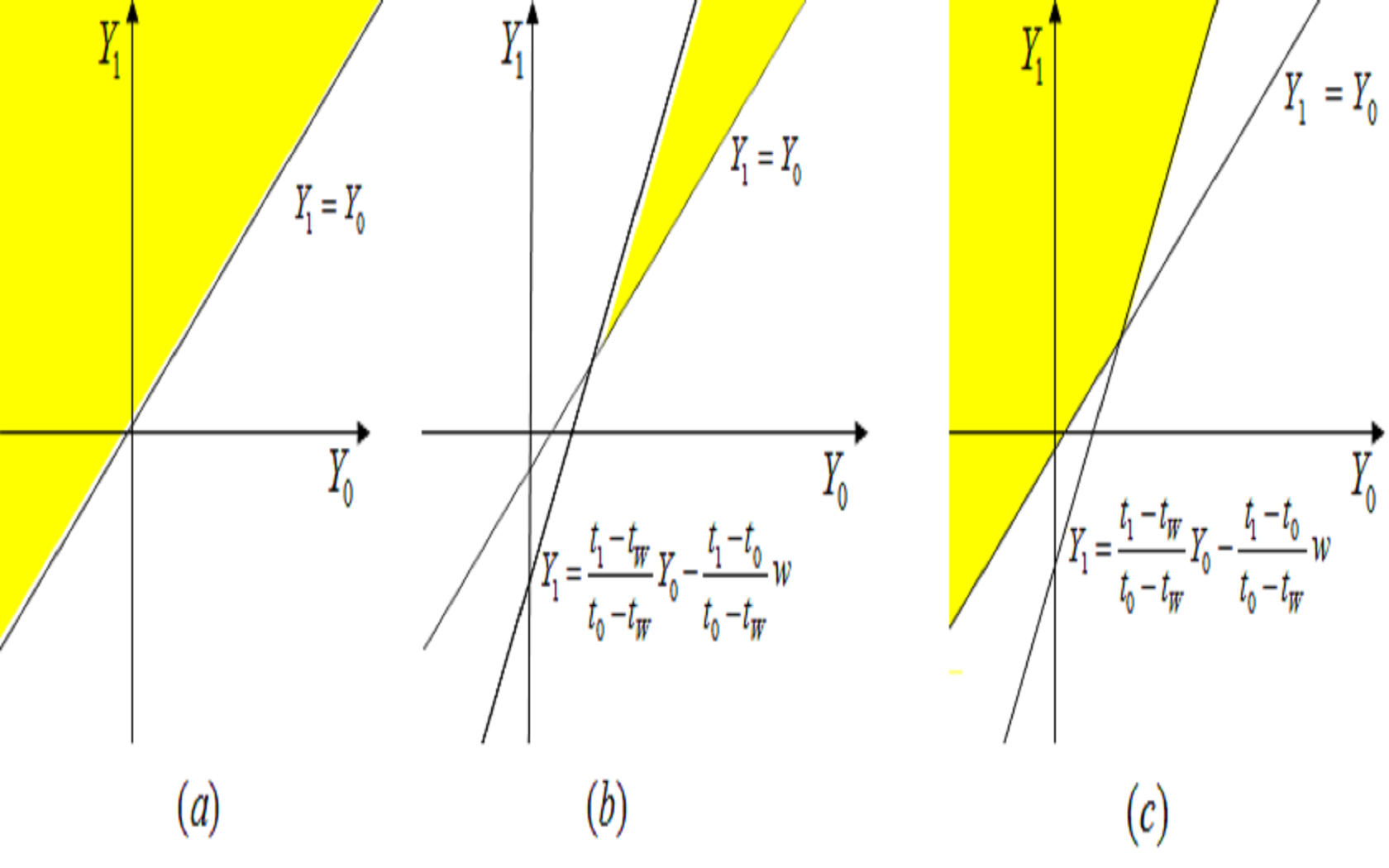
Figure 1: (a) MTR, (b) concave treatment response, (c) convex treatment response

Example 1

(Monotone Treatment Response) MTR only requires that the potential outcomes be weakly monotone in treatment with probability one:

$$\Pr\left(Y_{1}\geq Y_{0}\right)=1.$$

MTR restricts the support of $(Y_{0},Y_{1})$ to the region above the straight line $Y_{1}=Y_{0},$ as shown in Figure 1(a).

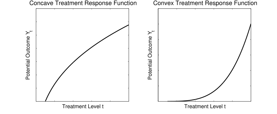
Figure 2: Concave treatment response and convex treatment response

Example 2

(Concave/Convex Treatment Response) Consider panel data where the outcome without treatment and an outcome either with the low-intensity treatment or with the high-intensity treatment is observed for each individual. Let $W$ denote the observed outcome without treatment, while $Y_{0}$ and $Y_{1}$ denote potential outcomes under low-intensity treatment and high-intensity treatment, respectively. Suppose that the treatment response function is nondecreasing and that either $\left(W,Y_{0}\right)$ or $\left(W,Y_{1}\right)$ is observed for each individual. Concavity and convexity of the treatment response function imply $\Pr\left(\frac{Y_{0}-W}{t_{0}-t_{W}}\geq\frac{Y_{1}-Y_{0}}{t_{1}-t_{0}},Y_{1}\geq Y_{0}\geq W\right)=1$ and $\Pr\left(\frac{Y_{0}-W}{t_{0}-t_{W}}\geq\frac{Y_{1}-Y_{0}}{t_{1}-t_{0}},Y_{1}\geq Y_{0}\geq W\right)=1$, respectively, where $t_{d}$ is a level of input for each treatment status $d\in\left\{0,1\right\}$ while $t_{W}$ is a level of input without the treatment and $t_{W}<t_{0}<t_{1}$.  Given $W=w,$ concavity and convexity of the treatment response function restrict the support of $(Y_{0},Y_{1})$ to the region below the straight line $Y_{1}=\frac{t_{1}-t_{W}}{t_{0}-t_{W}}Y_{0}-\frac{t_{1}-t_{0}}{t_{0}-t_{W}}w$ and above the straight line $Y_{1}=Y_{0}$, and to the region above two straight lines $Y_{1}=\frac{t_{1}-t_{W}}{t_{0}-t_{W}}Y_{0}-\frac{t_{1}-t_{0}}{t_{0}-t_{W}}w$ and $Y_{1}=Y_{0},$ respectively, as shown in Figures 1(b) and (c).

Example 3

(Roy Model) In the Roy model, individuals self-select into treatment when their benefits from the treatment are greater than nonpecuniary costs for treatment participation. The extended Roy model assumes that the nonpecuniary cost is deterministic with the following selection equation:

$$D=\boldsymbol{1}\left\{Y_{1}-Y_{0}\geq\mu_{C}\left(Z\right)\right\},$$

where $\mu_{C}\left(Z\right)$ represents nonpecuniary costs with a vector of observables $Z$. Then treated $(D=1)$ and untreated people $(D=0)$ are the observed groups satisfying support restrictions $\left\{Y_{1}-Y_{0}\geq\mu_{C}\left(Z\right)\right\}$ and $\left\{Y_{1}-Y_{0}<\mu_{C}\left(Z\right)\right\}$, respectively.

Example 4

(DTE conditional on Potential Outcomes) The conditional DTE for the unobservable subgroup whose potential outcomes belong to a certain set $C$ is written as

$$\Pr\left\{Y_{1}-Y_{0}\leq\delta|\left(Y_{0},Y_{1}\right)\in C\right\}.$$

For example, the distribution of the college premium for people whose potential wage without college degrees is less than or equal to $\theta$ can be written as

$$\Pr\left\{Y_{1}-Y_{0}\leq\delta|Y_{0}\leq\theta\right\},$$

where $Y_{0}$ and $Y_{1}$ denote the potential wage without and with college degrees, respectively.

2.2 DTE Bounds without Support Restrictions

Prior to considering support restrictions, I briefly discuss bounds on the DTE given marginal distributions without those restrictions.

Lemma 1

(Makarov (1981)) Let

$$F_{\Delta}^{L}\left(\delta\right) =\sup_{y}\max\left(F_{1}\left(y\right)-F_{0}\left(y-\delta\right),0\right),$$

$$F_{\Delta}^{U}\left(\delta\right) =1+\inf_{y}\min\left(F_{1}\left(y\right)-F_{0}\left(y-\delta\right),0\right).$$

Then for any $\delta\in\mathbb{R},$

$$F_{\Delta}^{L}\left(\delta\right)\leq F_{\Delta}\left(\delta\right)\leq F_{\Delta}^{U}\left(\delta\right),$$

and both $F_{\Delta}^{L}\left(\delta\right)$ and $F_{\Delta}^{U}\left(\delta\right)$ are sharp.

Henceforth, I call these bounds Makarov bounds. One way to bound the DTE is to use joint distribution bounds since the DTE can be obtained from the joint distribution. When the marginal distributions of $Y_{0}$ and $Y_{1}$ are given, Fréchet inequalities provide some information on their unknown joint distribution as follows: for any measurable sets $A_{0}$ and $A_{1}$ in $\mathbb{R}$,

$$\max\left\{\mu_{0}\left(A_{0}\right)+\mu_{1}\left(A_{1}\right)-1,0\right\}\leq\pi\left(A_{0}\times A_{1}\right)\leq\min\left\{\mu_{0}\left(A_{0}\right),\mu_{1}\left(A_{1}\right)\right\}.$$

Consider the event $\left\{Y_{0}\in A_{0},Y_{1}\in A_{1}\right\}$ for any interval $A_{d}=[a_{d},b_{d}]$ with $a_{d}<b_{d}$  and $d\in\left\{0,1\right\}.$ In  Figure 3, $\pi\left(A_{0}\times A_{1}\right)$ corresponds to the probability of the shaded rectangular region in the support space of $\left(Y_{0},Y_{1}\right).$ Note that since marginal distributions are defined in the one dimensional space, they are informative on the joint distribution for rectangular regions in the two-dimensional support space of $\left(Y_{0},Y_{1}\right)$, as illustrated in Figure 3.

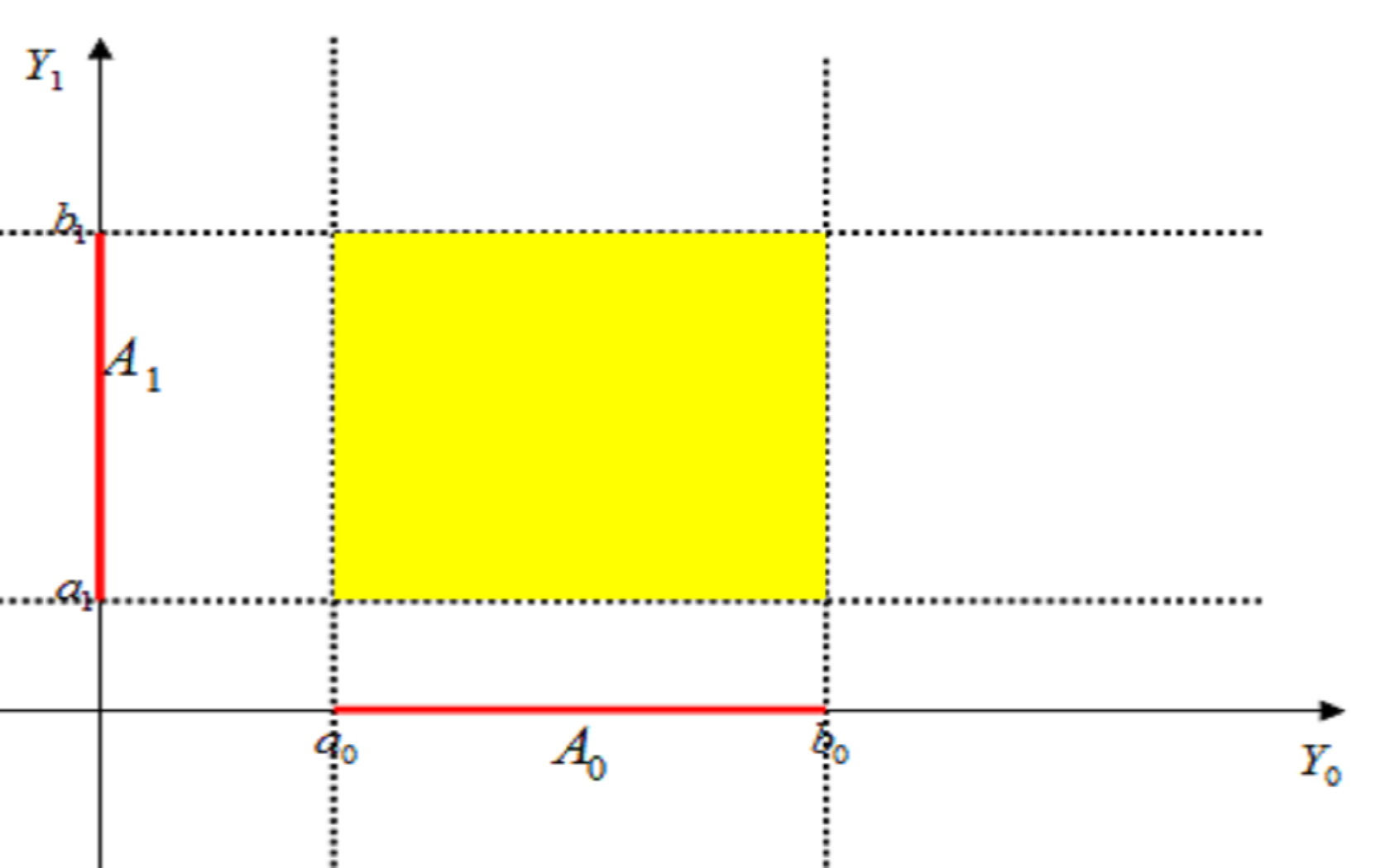
Figure 3: $\{Y_{0}\in A_{0},Y_{1}\in A_{1}\}$

Graphically, the DTE corresponds to the region below the straight line $Y_{1}=Y_{0}+\delta$ in the support space as shown in Figure 4. Since the given marginal distributions are informative on the joint distribution for rectangular regions in the support space, one can bound the DTE by considering two rectangles $\left\{Y_{0}\geq y-\delta,Y_{1}\leq y\right\}$ and $\left\{Y_{0}<y^{\prime}-\delta,Y_{1}>y^{\prime}\right\}$ for any $\left(y,y^{\prime}\right)\in\mathbb{R}^{2}.$ Although the probability of each rectangle is not point-identified, it can be bounded by Fréchet inequalities. Since the DTE is bounded from below by the Fréchet lower bound on $\Pr\left\{Y_{0}\geq y-\delta,Y_{1}\leq y\right\}$ for any $y\in\mathbb{R},$ the lower bound on the DTE is obtained as follows:

$$\underset{y}{\sup}\max\left(F_{1}\left(y\right)-F_{0}\left(y-\delta\right),0\right)\leq F_{\Delta}\left(\delta\right).$$

Similarly, the DTE is bounded from above by $1-\Pr\left\{Y_{0}<y^{\prime}-\delta,Y_{1}>y^{\prime}\right\}$ for any $y^{\prime}\in\mathbb{R}$. Therefore, the upper bound on the DTE is obtained by the Fréchet lower bound on $\Pr\left\{Y_{0}<y^{\prime}-\delta,Y_{1}>y^{\prime}\right\}$ as follows:

$$F_{\Delta}\left(\delta\right)\leq 1-\sup_{y}\max\left(F_{0}\left(y-\delta\right)-F_{1}\left(y\right),0\right).$$

Makarov (1981) proved that those lower and upper bounds are sharp.

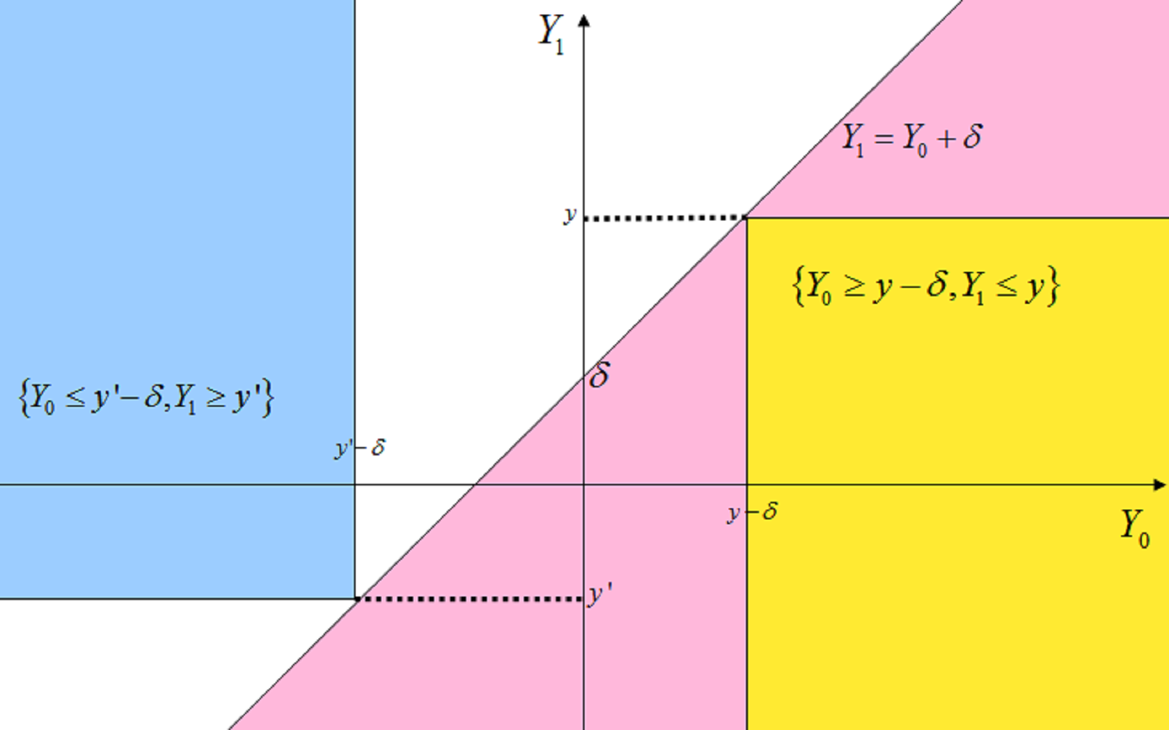
Figure 4: Makarov bounds

If the marginal distributions of $Y_{0}$ and $Y_{1}$ are both absolutely continuous with respect to the Lebesgue measure on $\mathbb{R}$, then the Makarov upper bound and lower bound are achieved when $F\left(y_{0},y_{1}\right)=C_{s}^{L}\left(F_{0}\left(y_{0}\right),F_{1}\left(y_{1}\right)\right)$ and when $F\left(y_{0},y_{1}\right)=C_{t}^{U}\left(F_{0}\left(y_{0}\right),F_{1}\left(y_{1}\right)\right)$ respectively, where

$$s =F_{\Delta}^{U}\left(\delta\right)\text{ and }t=F_{\Delta}^{L}\left(\delta^{-}\right),$$

$$C_{s}^{U}\left(u,v\right) =\left\{\begin{array}[c]{ll}\min\left(u+s-1,v\right),&\text{ }1-s\leq u\leq 1,0\leq v\leq s,\\ \max\left(u+v-1,0\right),&\text{ elsewhere,}\end{array}\right.$$

$$C_{t}^{L}\left(u,v\right) =\left\{\begin{tabular}[c]{ll}$\min\left(u,v-t\right),$&$0\leq u\leq 1-t,t\leq v\leq 1,$\\ $\max\left(u+v-1,0\right),$&elsewhere.\end{tabular}\right.$$

Note that both $C_{s}^{U}\left(u,v\right)$ and $C_{t}^{L}\left(u,v\right)$ depend on $\delta$, through $s$ and $t$, respectively. Since the joint distribution achieving Makarov bounds varies with $\delta,$ Makarov bounds are only pointwise sharp, not uniformly. To address this issue, Firpo and Ridder (2008) proposed joint bounds on the DTE for multiple values of $\delta$, which are tighter than Makarov bounds. However, their improved bounds are not sharp and sharp bounds on the functional $F_{\Delta}$ are an open question. For details, see Frank et al. (1997), Nelsen (2006) and Firpo and Ridder (2008).

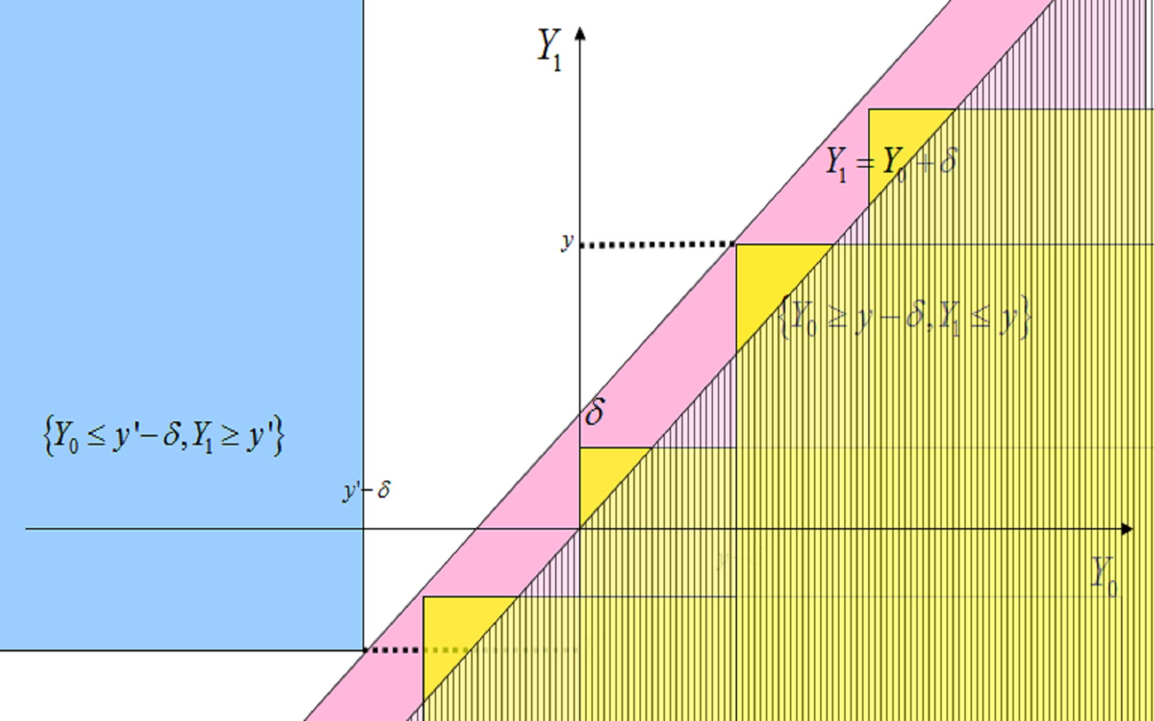
Figure 5: Makarov bounds are not best possible under MTR

Although Makarov bounds are sharp when no other restrictions are imposed, they are often too wide to be informative in practice and not sharp in the presence of additional restrictions on the set of possible pairs of potential outcomes. Figure 5 illustrates that if the support is restricted to the region above the straight line $Y_{1}=Y_{0}$ by MTR, the Makarov lower bound is not the best possible anymore. The lower bound can be improved under MTR because MTR allows multiple mutually exclusive rectangles to be placed below the straight line $Y_{1}=Y_{0}+\delta$.

Methods of establishing sharp bounds under this class of restrictions and fixed marginal distributions have remained unanswered in the literature. The central difficulty lies in finding out the particular joint distributions achieving sharp bounds among all joint distributions that have the given marginal distributions and satisfy support restrictions. The next subsection shows that an optimal transportation approach circumvents this difficulty through its dual formulation.

2.3 Optimal Transportation Approach

An optimal transportation problem was first formulated by Monge (1781) who studied the most efficient way to move a given distribution of mass to another distribution in a different location. Much later Monge’s problem was rediscovered and developed by Kantorovich. The optimal transportation problem of Monge-Kantorovich type is posed as follows. Let $c\left(y_{0},y_{1}\right)$ be a nonnegative lower semicontinuous function on $\mathbb{R}^{2}$ and define $\Pi\left(\mu_{0},\mu_{1}\right)$ to be the set of joint distributions on $\mathbb{R}^{2}$ that have $\mu_{0}$ and $\mu_{1}$ as marginal distributions. The optimal transportation problem solves

$$\underset{\pi\in\Pi\left(\mu_{0},\mu_{1}\right)}{\inf}\int c\left(y_{0},y_{1}\right)d\pi.$$ (2)

The objective function in the minimization problem is linear in the joint distribution $\pi$ and the constraint is that the joint distribution $\pi$ should have fixed marginal distributions $\mu_{0}$ and $\mu_{1}$. $c\left(y_{0},y_{1}\right)$ and $\int c\left(y_{0},y_{1}\right)d\pi$ are called the cost function and the total cost, respectively. Kantorovich (1942) developed a dual formulation for the problem (2), which is a key feature of the optimal transportation approach.

Lemma 2

(Kantorovich duality) Let $c:\mathbb{R}\times\mathbb{R}\rightarrow\left[0,\infty\right]$ be a lower semicontinuous function and $\Phi_{c}$ the set of all functions $\left(\varphi,\psi\right)\in L^{1}\left(d\mu_{0}\right)$ $\times L^{1}\left(d\mu_{1}\right)$ with

$$\varphi\left(y_{0}\right)+\psi\left(y_{1}\right)\leq c\left(y_{0},y_{1}\right)$$ (3)

Then,

$$\underset{\pi\in\Pi\left(\mu_{0},\mu_{1}\right)}{\inf}\int c\left(y_{0},y_{1}\right)d\pi=\underset{\left(\varphi,\psi\right)\in\Phi_{c}}{\sup}\left(\int\varphi\left(y_{0}\right)d\mu_{0}+\int\psi\left(y_{1}\right)d\mu_{1}\right).$$ (4)

Also, the infimum in the left-hand side of (4) and the supremum in the right-hand side of (4) are both attainable, and the value of the supremum in the right-hand side does not change if one restricts $\left(\varphi,\psi\right)$ to be bounded and continuous.

Remark 1

Note that the cost function $c\left(y_{0},y_{1}\right)$ may be infinite for some $\left(y_{0},y_{1}\right)\in\mathbb{R}^{2}.$ Since $c$ is a nonnegative function, the integral $\int c\left(y_{0},y_{1}\right)d\pi\in\left[0,\infty\right]$ is well-defined.

This dual formulation provides a key to solve the optimization problem (2); I can overcome the difficulty associated with picking the maximizer joint distribution in the set $\Pi\left(\mu_{0},\mu_{1}\right)$ by solving optimization with respect to given marginal distributions. The dual functions $\varphi\left(y_{0}\right)$ and $\psi\left(y_{1}\right)$ are Lagrange multipliers corresponding to the constraints $\pi\left(y_{0}\times\mathbb{R}\right)=\mu_{0}\left(y_{0}\right)$ and $\pi\left(\mathbb{R}\times y_{1}\right)=\mu_{1}\left(y_{1}\right),$ respectively, for each $y_{0}$ and $y_{1}$ in $\mathcal{Y}_{0}$ and $\mathcal{Y}_{1}$. Henceforth they are both assumed to be bounded and continuous without loss of generality. By the condition (3), each pair $\left(\varphi,\psi\right)$ in $\Phi_{c}$ satisfies

$$\varphi\left(y_{0}\right) \leq\underset{y_{1}\in\mathbb{R}}{\inf}\left\{c\left(y_{0},y_{1}\right)-\psi\left(y_{1}\right)\right\},$$ (5)

$$\psi\left(y_{1}\right) \leq\underset{y_{0}\in\mathbb{R}}{\inf}\left\{c\left(y_{0},y_{1}\right)-\varphi\left(y_{0}\right)\right\}.$$

At the optimum for $\left(y_{0},y_{1}\right)$ in the support of the optimal joint distribution, the inequality in (3) holds with equality and there exists a pair of dual functions $\left(\varphi,\psi\right)$ that satisfies both inequalities in (5) with equalities.

In recent years, this dual formulation has turned out to be powerful and useful for various problems related to the equilibrium and decentralization in economics. See Ekeland (2005, 2010), Carlier (2010), Chiappori et al. (2010), Chernozhukov et al. (2010), and Galichon and Salanié (2012). In econometrics, Galichon and Henry (2009) and Ekeland et al. (2010) showed that the dual formulation yields a test statistic for a set of theoretical restrictions in partially identified economic models. They set the cost function as an indicator for incompatibility of the structure with the data and derived a  Kolmogorov Smirnov type test statistic from a well known dual representation theorem; see Lemma 3 below. Similarly, Galichon and Henry (2011) showed that the identified set of structural parameters in game theoretic models with pure strategy equilibria can be formulated as an optimal transportation problem using the $\{0,1\}$-valued cost function.

Establishing sharp bounds on the DTE is also an optimal transportation problem with an indicator function as the cost function. The DTE can be written as the integration of an indicator function with respect to the joint distribution $\pi$ as follows:

$$F_{\Delta}\left(\delta\right)=\Pr\left(Y_{1}-Y_{0}<\delta\right)=\int\boldsymbol{1}\left\{y_{1}-y_{0}<\delta\right\}d\pi.$$

Since marginal distributions of potential outcomes are given as $\mu_{0}$ and $\mu_{1},$ establishing sharp bounds reduces to picking a particular joint distribution maximizing or minimizing the DTE from all possible joint distributions having $\mu_{0}$ and $\mu_{1}$ as their marginal distributions. Then the DTE is bounded as follows:

$$\underset{\pi\in\Pi\left(\mu_{0},\mu_{1}\right)}{\inf}\int\boldsymbol{1}\left\{y_{1}-y_{0}<\delta\right\}d\pi\leq F_{\Delta}\left(\delta\right)\leq\underset{\pi\in\Pi\left(\mu_{0},\mu_{1}\right)}{\sup}\int\boldsymbol{1}\left\{y_{1}-y_{0}\leq\delta\right\}d\pi,$$

where $\Pi\left(\mu_{0},\mu_{1}\right)$ is the set of joint distributions that have $\mu_{0}$ and $\mu_{1}$ as marginal distributions. For the indicator function, the Kantorovich duality lemma for $\{0,1\}-$valued costs in Villani (2003) can be applied as follows:

Lemma 3

(Kantorovich duality for $\{0,1\}$-valued costs) The sharp lower bound on the DTE has the following dual representation:

$$\underset{\pi\in\Pi\left(\mu_{0},\mu_{1}\right)}{\inf}\int\boldsymbol{1}\left\{y_{1}-y_{0}<\delta\right\}d\pi$$ (6)

$$=\sup_{A\subset\mathbb{R}}\left\{\mu_{0}\left(A\right)-\mu_{1}\left(A^{D}\right);\text{ }A\text{ is closed}\right\}$$

where

$$A^{D}=\left\{y_{1}\in\mathbb{R}|\exists y_{0}\in A\text{ s.t. }y_{1}-y_{0}\geq\delta\right\}.$$

Similarly, the sharp upper bound on the DTE can be written as follows:

$$\underset{\pi\in\Pi\left(\mu_{0},\mu_{1}\right)}{\sup}\int\boldsymbol{1}\left\{y_{1}-y_{0}\leq\delta\right\}d\pi$$

$$=1-\underset{F\in\Pi\left(F_{0},F_{1}\right)}{\inf}\int\boldsymbol{1}\left\{y_{1}-y_{0}>\delta\right\}d\pi$$

$$=1-\sup_{A\subset\mathbb{R}}\left\{\mu_{0}\left(A\right)-\mu_{1}\left(A^{E}\right);\text{ }A\text{ is closed}\right\}$$

where

$$A^{E}=\left\{y_{1}\in\mathbb{R}|\exists y_{0}\in A\text{ s.t. }y_{1}-y_{0}\leq\delta\right\}.$$

Proof. See pp. $44-46$ of Villani (2003).   

In the following discussion, I focus on the lower bound on the DTE since the procedure to obtain the upper bound is similar.

Remark 2

In the proof of Lemma 3, Villani (2003) showed that at the optimum, $A=\left\{x\in\mathbb{R}|\varphi\left(x\right)\geq s\right\}$ for some $s\in\left[0,1\right]$. Since the function $\varphi$ is continuous, if $\varphi$ is nondecreasing then $A=[a,\infty)$ for some $a\in\left[\mathbb{-\infty},\mathbb{\infty}\right]$ where $A=\phi$ if $a=\mathbb{\infty}.$ In contrast, if $\varphi$ is nonincreasing, then $A=(-\infty,a]$ where $A=\phi$ if $a=-\mathbb{\infty}$

Remember that for any $\left(y_{0},y_{1}\right)$ in the support of the optimal joint distribution, $\varphi$ and $\psi$ satisfy

$$\varphi\left(y_{0}\right)=\underset{y_{1}\in\mathbb{R}}{\inf}\left\{\boldsymbol{1}\left\{y_{1}-y_{0}<\delta\right\}-\psi\left(y_{1}\right)\right\}.$$ (7)

Pick $\left(y_{0}^{\prime},y_{1}^{\prime}\right)$ and $\left(y_{0}^{\prime\prime},y_{1}^{\prime\prime}\right)$ with $y_{0}^{\prime\prime}>y_{0}^{\prime}$ in the support of the optimal joint distribution. Then,

$$\varphi\left(y_{0}^{\prime}\right) =\boldsymbol{1}\left\{y_{1}^{\prime}-y_{0}^{\prime}<\delta\right\}-\psi\left(y_{1}^{\prime}\right)$$ (8)

$$\leq\boldsymbol{1}\left\{y_{1}^{\prime\prime}-y_{0}^{\prime}<\delta\right\}-\psi\left(y_{1}^{\prime\prime}\right)$$

$$\leq\boldsymbol{1}\left\{y_{1}^{\prime\prime}-y_{0}^{\prime\prime}<\delta\right\}-\psi\left(y_{1}^{\prime\prime}\right)$$

$$=\varphi\left(y_{0}^{\prime\prime}\right).$$

The inequality in the second line of (8) is obvious from (7) and the inequality in the third line of (8) holds because $\boldsymbol{1}\left\{y_{1}-y_{0}<\delta\right\}$ is nondecreasing in $y_{0}$. Since $\varphi$ is nondecreasing on the set $\left\{y_{0}\in\mathcal{Y}_{0}|\exists y_{1}\in\mathcal{Y}_{1}\text{ s.t. }\left(y_{0},y_{1}\right)\in Supp\left(\pi\right)\right\}$, by Remark 2 $A$ can be written as $[a,\infty)$ for some $a\in\left[\mathbb{-\infty},\mathbb{\infty}\right].$

Figure 6: $A^{D}$ for $A=[a,\infty)$

As shown in Figure 6, $A^{D}=\phi$ for $A=\phi,$ and $A^{D}=[a+\delta,\infty)$ for $A=[a,\infty)$ with $a\in\left(-\infty,\infty\right)$. Then, $\mu_{0}\left(A\right)-\mu_{1}\left(A^{D}\right)=0$ for $A=\phi$, while $\mu_{0}\left(A\right)-\mu_{1}\left(A^{D}\right)=F_{1}\left(a+\delta\right)-F_{0}\left(a\right)$ for $A=[a,\infty).$ Therefore, the RHS in (6) reduces to

$$\underset{a\in\mathbb{R}}{\sup}\max\left[F_{1}\left(a+\delta\right)-F_{0}\left(a\right),0\right],$$

which is equal to the Makarov lower bound. One can derive the Makarov upper bound in the same way.

Now consider the support restriction $\Pr\left(\left(Y_{0},Y_{1}\right)\in C\right)=1$. Note that this restriction is linear in the entire joint distribution $\pi,$ since it can be rewritten as $\int\boldsymbol{1}_{C}\left(y_{0},y_{1}\right)d\pi=1$. The linearity makes it possible to handle this restriction with penalty. In particular, since support restrictions hold with probability one, the corresponding penalty is infinite. Therefore, one can embed $1-\boldsymbol{1}_{C}\left(y_{0},y_{1}\right)$ into the cost function with an infinite multiplier $\lambda=\infty$ as follows:

$$\underset{\pi\in\Pi\left(\mu_{0},\mu_{1}\right)}{\inf}\int\left\{\boldsymbol{1}\left\{y_{1}-y_{0}<\delta\right\}+\lambda\left(1-\boldsymbol{1}_{C}\left(y_{0},y_{1}\right)\right)\right\}d\pi$$ (9)

The minimization problem (9) is well defined with $\lambda=\infty$ as noted in Remark 1. Note that for $\lambda=\infty,$ any joint distribution which violates the restriction $\Pr\left(\left(Y_{0},Y_{1}\right)\in C\right)=1$ would cause infinite total costs in (9) and it is obviously excluded from the potential optimal joint distribution candidates. The optimal joint distribution should thus satisfy the restriction $\Pr\left(\left(Y_{0},Y_{1}\right)\in C\right)=1$ to avoid infinite costs by not permitting any positive probability density for the region outside of the set $C$. Similarly, the upper bound on the DTE is written as

$$\underset{\pi\in\Pi\left(\mu_{0},\mu_{1}\right)}{\sup}\int\left\{\boldsymbol{1}\left\{y_{1}-y_{0}\leq\delta\right\}-\lambda\left(1-\boldsymbol{1}_{C}\left(y_{0},y_{1}\right)\right)\right\}d\pi$$ (10)

$$=1-\underset{\pi\in\Pi\left(\mu_{0},\mu_{1}\right)}{\inf}\int\left\{\boldsymbol{1}\left\{y_{1}-y_{0}>\delta\right\}+\lambda\left(1-\boldsymbol{1}_{C}\left(y_{0},y_{1}\right)\right)\right\}d\pi.$$

To the best of my knowledge, this is the first paper that allows for $\left\{0,1,\infty\right\}$-valued costs. Although the econometrics literature based on the optimal transportation approach has used Lemma 3 for $\{0,1\}-$valued costs, the problem (9) cannot be solved using Lemma 3. In the next section, I develop a dual representation for (9) in order to characterize sharp bounds on the DTE.

3 Main Results

This section characterizes sharp DTE bounds under general support restrictions by developing a dual representation for problems (9) and (10). I use this characterization to derive sharp DTE bounds for various economic examples. Also, I provide intuition regarding improvement of the identification region via graphical illustrations.

3.1 Characterization

The following theorem is the main result of the paper.

Theorem 1

The sharp lower and upper bounds on the DTE under $\Pr\left(\left(Y_{0},Y_{1}\right)\in C\right)=1$ are characterized as follows: for any $\delta\in\mathbb{R},$

$$F_{\Delta}^{L}\left(\delta\right)\leq F_{\Delta}\left(\delta\right)\leq F_{\Delta}^{U}\left(\delta\right),$$

where

$$F_{\Delta}^{L}\left(\delta\right) =\underset{\left\{A_{k}\right\}_{k=-\infty}^{\infty}}{\sup}\sum\limits_{k=-\infty}^{\infty}\max\left\{\mu_{0}\left(A_{k}\right)-\mu_{1}\left(A_{k}^{C}\right),0\right\},$$ (11)

$$F_{\Delta}^{U}\left(\delta\right) =1-\underset{\left\{B_{k}\right\}_{k=-\infty}^{\infty}}{\sup}\sum\limits_{k=-\infty}^{\infty}\max\left\{\mu_{0}\left(B_{k}\right)-\mu_{1}\left(B_{k}^{C}\right),0\right\},$$

where

$$\left\{A_{k}\right\}_{k=-\infty}^{\infty}\text{ and }\left\{B_{k}\right\}_{k=-\infty}^{\infty}\text{ are both monotonically decreasing sequences of open sets,}$$

$$A_{k}^{C} =\begin{tabular}[c]{l}$\left\{y_{1}\in\mathbb{R}|\exists y_{0}\in A_{k}\text{ s.t. }y_{1}-y_{0}\geq\delta\text{ and }\left(y_{0},y_{1}\right)\in C\right\}$\\ $\cup\left\{y_{1}\in\mathbb{R}|\exists y_{0}\in A_{k+1}\text{ s.t. }y_{1}-y_{0}<\delta\text{ and }\left(y_{0},y_{1}\right)\in C\right\}$,\end{tabular}$$

$$B_{k}^{C} =\begin{tabular}[c]{l}$\left\{y_{1}\in\mathbb{R}|\exists y_{0}\in B_{k}\text{ s.t. }y_{1}-y_{0}\leq\delta\text{ and }\left(y_{0},y_{1}\right)\in C\right\}$\\ $\cup\left\{y_{1}\in\mathbb{R}|\exists y_{0}\in B_{k+1}\text{ s.t. }y_{1}-y_{0}>\delta\text{ and }\left(y_{0},y_{1}\right)\in C\right\}\text{ for any integer }k.$\end{tabular}$$

Proof. See Appendix A.   

Theorem 1 is obtained by applying Kantorovich duality in Lemma 2 to the optimal transportation problems (9) and (10). Note that the sharpness of the bounds is also confirmed by Lemma 2. Since characterization of the upper bound is similar to that of the lower bound, I maintain the focus of the discussion on the lower bound. The minimization problem (9) can be written in the dual formulation as follows: for $\lambda=\infty,$

$$\underset{\pi\in\Pi\left(\mu_{0},\mu_{1}\right)}{\inf}\int\left\{\boldsymbol{1}\left\{y_{1}-y_{0}<\delta\right\}+\lambda\left(1-\boldsymbol{1}_{C}\left(y_{0},y_{1}\right)\right)\right\}d\pi$$

$$=\underset{\left(\varphi,\psi\right)\in\Phi_{c}}{\sup}\left(\int\varphi\left(y_{0}\right)d\mu_{0}+\int\psi\left(y_{1}\right)d\mu_{1}\right),$$

where

$$\Phi_{c}=\left\{\left(\varphi,\psi\right);\text{ }\varphi\left(y_{0}\right)+\psi\left(y_{1}\right)\leq\boldsymbol{1}\left\{y_{1}-y_{0}<\delta\right\}+\lambda\left(1-\boldsymbol{1}_{C}\left(y_{0},y_{1}\right)\right)\text{ with }\lambda=\infty\right\}.$$

Note that at the optimum $\varphi\left(y_{0}\right)+\psi\left(y_{1}\right)=\boldsymbol{1}\left\{y_{1}-y_{0}<\delta\right\}$ for any $\left(y_{0},y_{1}\right)$ in the support of the optimal joint distribution. Therefore, dual functions $\varphi$ and $\psi$ can be written as follows: for any $\left(y_{0},y_{1}\right)$ in the support of the optimal joint distribution,

$$\varphi\left(y_{0}\right)=\underset{y_{1}:\left(y_{0},y_{1}\right)\in C}{\inf}\left\{\boldsymbol{1}\left\{y_{1}-y_{0}<\delta\right\}-\psi\left(y_{1}\right)\right\}.$$

In my proof of Theorem 1, $A_{k}$ is defined as $A_{k}=\left\{x\in\mathbb{R}:\varphi(x)>s+k\right\}$ for the function $\varphi$, some $s\in[0,1],$ and each integer $k.$ Since the dual function $\varphi$ is continuous, if $\varphi$ is nondecreasing then $A_{k}$ $=(a_{k},\infty)$ for some $a_{k}\in\left[-\infty,\infty\right].$ Note that $A_{k}=\phi$ for $a_{k}=\infty.$ Also, since $\left\{A_{k}\right\}_{k=-\infty}^{\infty}$ is a monotonically decreasing sequence of open sets, $a_{k}\leq a_{k+1}$ for every integer $k.$ In contrast, if $\varphi$ is nonincreasing at the optimum then $A_{k}=(-\infty,a_{k})$ for $a_{k}\in\left[-\infty,\infty\right]$ and $a_{k+1}\leq a_{k}$ for each integer $k$. Note that $A_{k}=\phi$ for $a_{k}=-\infty$. In the next subsection, I will show that the function $\varphi$ is monotone for economic examples considered in this paper and that sharp DTE bounds in each example are readily derived from monotonicity of $\varphi$.

Remark 3

(Robustness of the sharp bounds) My sharp DTE bounds are robust for support restrictions in the sense that they do not rely too heavily on the small deviation of the restriction. I can verify this by showing that sharp bounds under $\Pr\left(\left(Y_{0},Y_{1}\right)\in C\right)\geq p$ converge to those under $\Pr\left(\left(Y_{0},Y_{1}\right)\in C\right)=1,$ as $p$ goes to one. The sharp lower bound under $\Pr\left(\left(Y_{0},Y_{1}\right)\in C\right)\geq p$ can be obtained with a multiplier $\widetilde{\lambda}_{p}\geq 0$ as follows:

$$F_{\Delta}^{L}\left(\delta\right)=\underset{\pi\in\Pi\left(\mu_{0},\mu_{1}\right)}{\inf}\int\left\{\boldsymbol{1}\left\{y_{1}-y_{0}<\delta\right\}+\widetilde{\lambda}_{p}\left(1-\boldsymbol{1}_{C}\left(y_{0},y_{1}\right)\right)\right\}d\pi.$$ (12)

Obviously, $\widetilde{\lambda}_{0}=0$. Furthermore, $\widetilde{\lambda}_{p}\leq\widetilde{\lambda}_{q}$ for $0\leq p<q\leq 1$ since $F_{\Delta}^{L}\left(\delta\right)$ is nondecreasing in $p.$ The proof of Theorem 1 can be easily adapted to the more general case in which the multiplier is given as a positive integer. If $\widetilde{\lambda}_{p}=2K$ in (12) for some positive integer $K$, then the dual representation reduces to

$$\underset{\left\{A_{k}\right\}_{k=-\infty}^{\infty}}{\sup}\sum\limits_{-\left(K-1\right)}^{K}\max\left\{\mu_{0}\left(A_{k}\right)-\mu_{1}\left(A_{k}^{C}\right),0\right\},$$

where $\left\{A_{k}\right\}_{k=-\left(K-1\right)}^{K}$ is monotonically decreasing. As $K$ goes to infinity, this obviously converges to the dual representation for the infinite Lagrange multiplier, which is given in (11).

3.2 Economic Examples

In this subsection, I derive sharp bounds on the DTE for concrete economic examples from the general characterization in Theorem 1.  As economic examples, MTR, concave treatment response, convex treatment response, and the Roy model of self-selection are discussed.

3.2.1 Monotone Treatment Response

Since the seminal work of Manski (1997), it has been widely recognized that MTR has an interesting identifying power for treatment effects parameters. MTR only requires that the potential outcomes be weakly monotone in treatment with probability one:

$$\Pr\left(Y_{1}\geq Y_{0}\right)=1.$$

His bounds on the DTE under MTR are obtained as follows: for $\delta<0,$ $F_{\Delta}\left(\delta\right)=0,$ and for $\delta\geq 0,$

$$\Pr\left(Y-y_{0}^{L}\leq\delta|D=1\right)p+\Pr\left(y_{1}^{U}-Y\leq\delta|D=0\right)\left(1-p\right)\leq F_{\Delta}\left(\delta\right)\leq 1,$$

where $p=\Pr\left(D=1\right),$ and $y_{0}^{L}$  is the support infimum of $Y_{0}$ while $y_{1}^{U}$  is the support supremum of $Y_{1}.$ He did not impose any other condition such as given marginal distributions of $Y_{0}$ and $Y_{1}$. Note that MTR has no identifying power on the DTE in the binary treatment setting without additional information. Since MTR restricts only the lowest possible value of $Y_{1}-Y_{0}$ as zero, the upper bound is trivially obtained as one for any $\delta\geq 0$. Similarly, MTR is uninformative for the lower bound, since MTR does not restrict the highest possible value of $Y_{1}-Y_{0}$. Furthermore, when the support of each potential outcome is given as $\mathbb{R}$, they yield completely uninformative upper and lower bounds $\left[0,1\right].$

However, I show that given marginal distribution functions $F_{0}$ and $F_{1}$, MTR has substantial identifying power for the lower bound on the DTE.

Corollary 1

Suppose that $\Pr\left(Y_{1}=Y_{0}\right)=0$. Under MTR, sharp bounds on the DTE are given as follows: for any $\delta\in\mathbb{R},$

$$F_{\Delta}^{L}\left(\delta\right)\leq F_{\Delta}\left(\delta\right)\leq F_{\Delta}^{U}\left(\delta\right),$$

where

$$F_{\Delta}^{U}\left(\delta\right) =\left\{\begin{array}[c]{cc}1+\underset{y\in\mathbb{R}}{\inf}\left\{\min\left(F_{1}\left(y\right)-F_{0}\left(y-\delta\right)\right),0\right\},&\text{for }\delta\geq 0,\\ 0,&\text{for }\delta<0.\end{array}\right.,$$

$$F_{\Delta}^{L}\left(\delta\right) =\left\{\begin{array}[c]{cc}\underset{\left\{a_{k}\right\}_{k=-\infty}^{\infty}\in\mathcal{A}_{\delta}}{\sup}\sum\limits_{k=-\infty}^{\infty}\max\left\{F_{1}\left(a_{k+1}\right)-F_{0}\left(a_{k}\right),0\right\},&\text{for }\delta\geq 0,\\ 0,&\text{for }\delta<0,\end{array}\right.,$$

$$\text{where }\mathcal{A}_{\delta} =\left\{\left\{a_{k}\right\}_{k=-\infty}^{\infty};0\leq a_{k+1}-a_{k}\leq\delta\text{ for each integer }k\right\}.$$

Proof. See Appendix A.   

The identifying power of MTR on the lower bound has an interesting graphical interpretation. As shown in Figure 7(a), the DTE under MTR corresponds to the probability of the region between two straight lines $Y_{1}=Y_{0}$ and $Y_{1}=Y_{0}+\delta$. Given marginal distributions, the Makarov lower bound is obtained by picking $y^{\ast}\in\mathbb{R}$ such that a rectangle $[y^{\ast}-\delta,\infty)\times(-\infty,y^{\ast}]$ yields the maximum Fréchet lower bound among all rectangles below the straight line $Y_{1}=Y_{0}+\delta.$ As shown in Figure 7(b), under MTR the probability of any rectangle $[y-\delta,\infty)\times(-\infty,y]$ below the straight line $Y_{1}=Y_{0}+\delta$ is equal to that of the triangle between two straight lines $Y_{1}=Y_{0}+\delta$ and $Y_{1}=Y_{0}.$ Now one can draw multiple mutually disjoint triangles between two straight lines $Y_{1}=Y_{0}$ and $Y_{1}=Y_{0}+\delta$ as in Figure 7(c). Since the probability of each triangle is equal to the probability of the rectangle extended to the right and bottom sides, the lower bound on each triangle is obtained by applying the Fréchet lower bound to the extended rectangle. Then the improved lower bound is obtained by summing the Fréchet  lower bounds on the triangles.

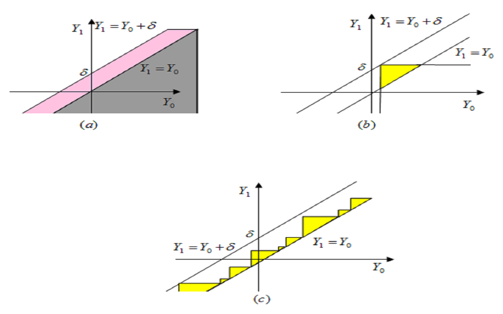
Figure 7: Improved lower bound under MTR

One of the key benefits of my characterization based on the optimal transportation approach is that it guarantees sharpness of the bounds. To show sharpness of given bounds in a copula approach, one should show what dependence structures achieve the bounds under fixed marginal distributions. This is technically difficult under MTR. However, the optimal transportation approach gets around this challenge by focusing on a dual representation involving given marginal distributions only.

Now I provide a sketch of the procedure to derive the lower bound under MTR from Theorem 1. The proof of deriving the lower bound from Theorem 1 proceeds in two stpng.

The first step is to show that the dual function $\varphi$ is nondecreasing so that one can put $A_{k}=(a_{k},\infty)$ for $a_{k}\in\left[-\infty,\infty\right]$ at the optimum. For any $\left(y_{0},y_{1}\right)$ in the support of the optimal joint distribution, the dual function $\varphi$ for the lower bound is written as

$$\varphi\left(y_{0}\right)=\underset{y_{1}\geq y_{0}}{\inf}\left\{\boldsymbol{1}\left\{y_{1}-y_{0}<\delta\right\}-\psi\left(y_{1}\right)\right\}.$$

For any $\left(y_{0}^{\prime},y_{1}^{\prime}\right)$ and $\left(y_{0}^{\prime\prime},y_{1}^{\prime\prime}\right)$ with $y_{0}^{\prime\prime}>y_{0}^{\prime}$ in the support of the optimal joint distribution,

$$\varphi\left(y_{0}^{\prime}\right) =\boldsymbol{1}\left\{y_{1}^{\prime}-y_{0}^{\prime}<\delta\right\}-\psi\left(y_{1}^{\prime}\right)$$

$$\leq\boldsymbol{1}\left\{y_{1}^{\prime\prime}-y_{0}^{\prime}<\delta\right\}-\psi\left(y_{1}^{\prime\prime}\right)$$

$$\leq\boldsymbol{1}\left\{y_{1}^{\prime\prime}-y_{0}^{\prime\prime}<\delta\right\}-\psi\left(y_{1}^{\prime\prime}\right)$$

$$=\varphi\left(y_{0}^{\prime\prime}\right).$$

The first inequality in the second line follows from $y_{1}^{\prime\prime}\geq y_{0}^{\prime\prime}>y_{0}^{\prime}$ The second inequality in the third line is satisfied because $\boldsymbol{1}\left\{y_{1}-y_{0}<\delta\right\}$ is nondecreasing in $y_{0}.$ Consequently, $\varphi$ is nondecreasing and thus $A_{k}=(a_{k},\infty)$ for $a_{k}\in[-\infty,\infty]$ at the optimum.

$A_{k}^{D}$ is obtained from $A_{k}$ as follows: for $\delta>0$ and $A_{k}=(a_{k},\infty)$ and $A_{k+1}=(a_{k+1},\infty),$

$$A_{k}^{D} =\left\{y_{1}\in\mathbb{R}|\exists y_{0}>a_{k}\text{ s.t. }\delta\leq y_{1}-y_{0}\right\}\cup\left\{y_{1}\in\mathbb{R}|\exists y_{0}>a_{k+1}\text{ s.t. }0\leq y_{1}-y_{0}<\delta\right\}$$

$$=\left(a_{k}+\delta,\infty\right)\cup\left(a_{k+1},\infty\right)$$

$$=\left(\min\left\{a_{k}+\delta,a_{k+1}\right\},\infty\right).$$

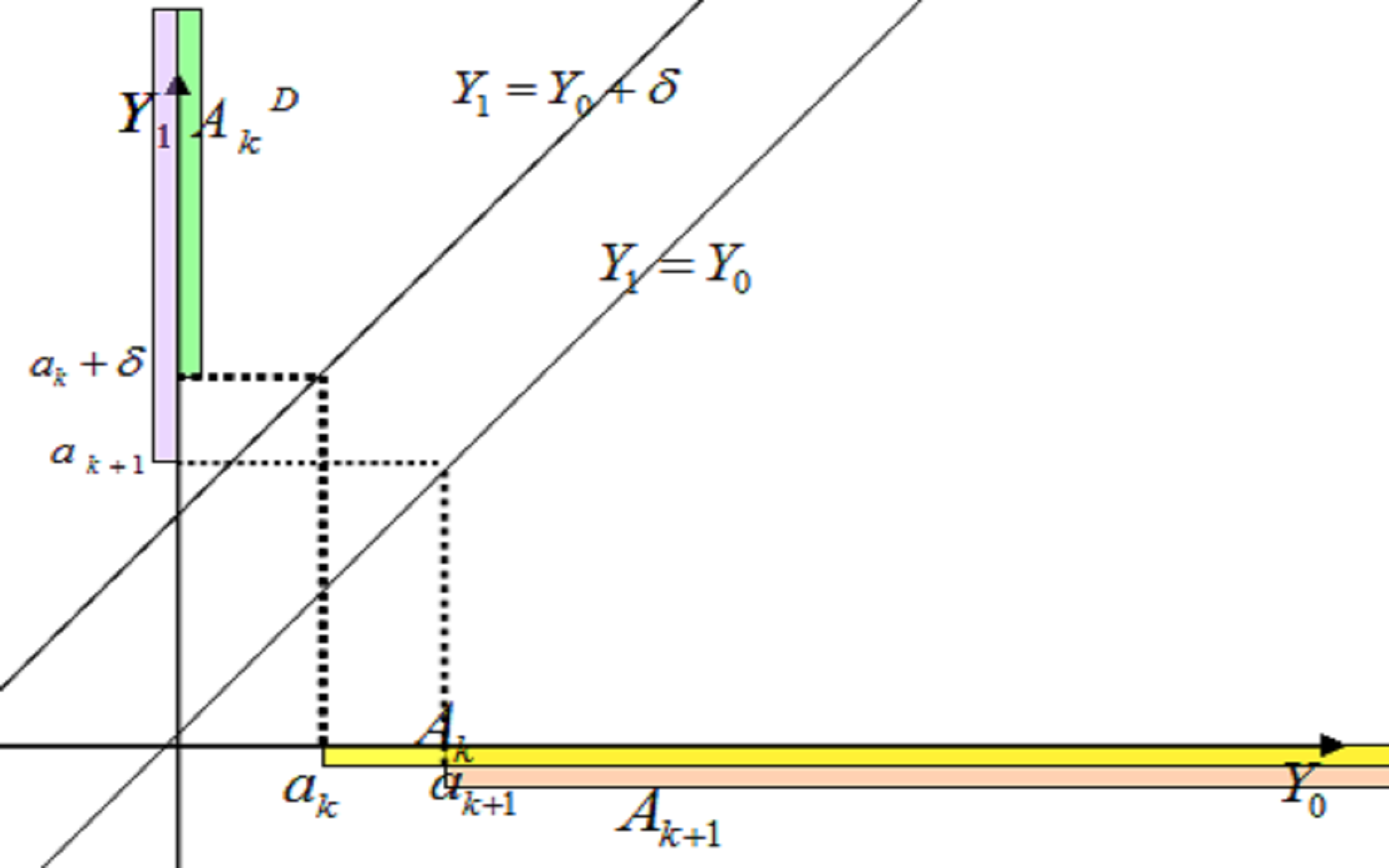
Figure 8: $A_{k}^{D}$ for $A_{k}=\left(a_{k},\infty\right)$ and $A_{k+1}=\left(a_{k+1},\infty\right).$

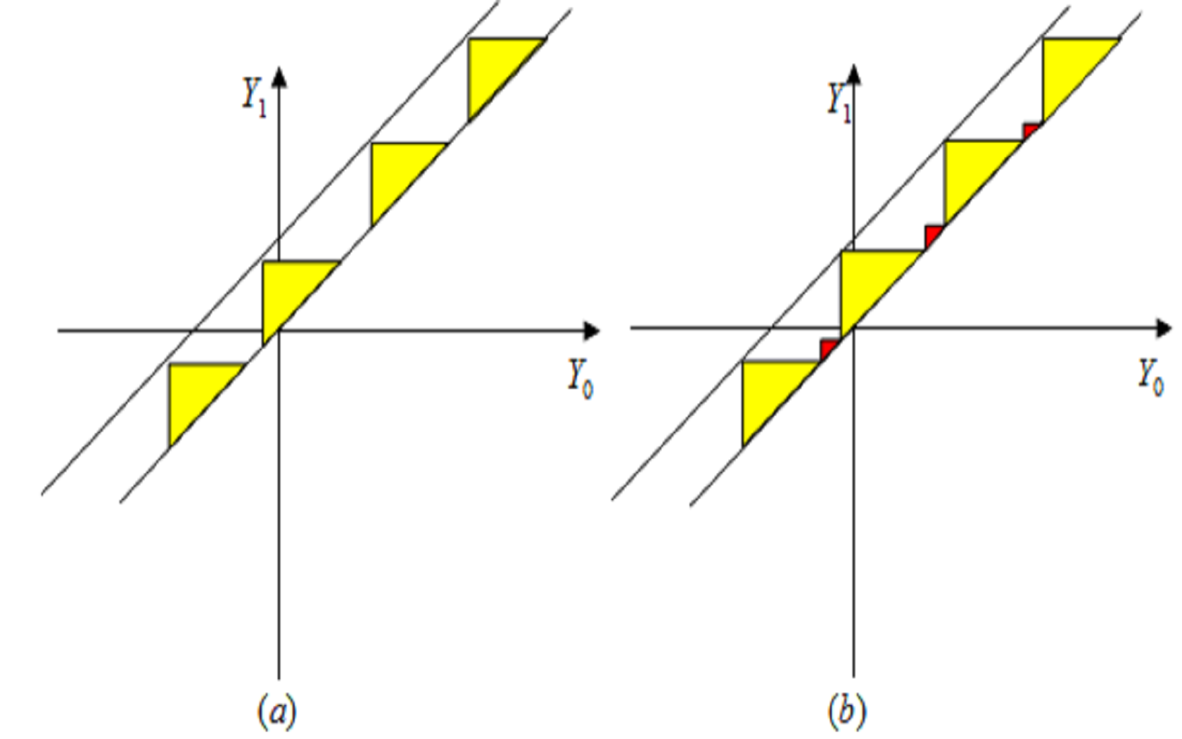
Figure 9: $a_{k+1}\leq a_{k}+\delta$ at the optimum

At the optimum, $\left\{a_{k}\right\}_{k=-\infty}^{\infty}$ should satisfy $a_{k+1}\leq a_{k}+\delta$ for each integer $k$. The rigorous proof is provided in Appendix A. I demonstrate this graphically here. As shown in Figure 7(c), my improved lower bound represents the sum of Fréchet lower bounds on the probability of a sequence of disjoint triangles. Suppose that $a_{k+1}>a_{k}+\delta$ for some integer $k$. This implies that triangles in the region between two straight lines $Y_{1}=Y_{0}+\delta$ and $Y_{1}=Y_{0}$ lie sparsely as shown in Figure 9(a). Then by adding extra triangles that fill the empty region between two sparse triangles as shown in Figure 9(b), one can always construct a sequence of mutually exclusive triangles that yield the identical or improved lower bound. Therefore, without loss of generality, one can assume $a_{k+1}\leq a_{k}+\delta$ for every integer $k$.

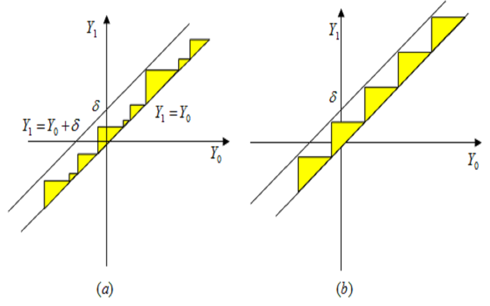
Figure 10: $a_{k+1}\leq a_{k}+\delta$ v.s. $a_{k+1}=a_{k}+\delta$

On the other hand, ones cannot exclude the case where $a_{k+1}<a_{k}+\delta$ for some integer $k$ at the optimum. This implies that for some $k,$ the triangle is not large enough to fit in the region corresponding to the DTE under MTR as shown in Figure 10(b). It depends on the underlying joint distribution which sequence of triangles would yield the tighter lower bound, and it is possible that $a_{k+1}<a_{k}+\delta$ for some integer $k$ at the optimum. Therefore,

$$A_{k}^{D} =\left(a_{k}+\delta,\infty\right)\cup\left(a_{k+1},\infty\right)$$

$$=\left(\min\left\{a_{k}+\delta,a_{k+1}\right\},\infty\right)$$

$$=\left(a_{k+1},\infty\right).$$

Consequently, for $\delta\geq 0,$

$$F_{\Delta}^{L}\left(\delta\right) =\underset{\left\{A_{k}\right\}_{k=-\infty}^{\infty}}{\sup}\sum\limits_{k=-\infty}^{\infty}\max\left\{\mu_{0}\left(A_{k}\right)-\mu_{1}\left(A_{k}^{D}\right),0\right\}$$

$$=\underset{\left\{a_{k}\right\}_{k=-\infty}^{\infty}}{\sup}\sum\limits_{k=-\infty}^{\infty}\max\left\{F_{1}\left(a_{k+1}\right)-F_{0}\left(a_{k}\right),0\right\}$$

where $0\leq a_{k+1}-a_{k}\leq\delta.$

3.2.2 Concave/Convex Treatment Response

Recall the setting of Example 2 in Subsection 2.1. Let $W$ denote the outcome without treatment and let $Y_{0}$ and $Y_{1}$ denote the potential outcomes with treatment at low-intensity, and with treatment at high-intensity, respectively. Let $t_{d}$ denote the level of input for each treatment status for $d=0,1,$ while $t_{W}$ is a level of input without the treatment with $t_{W}<t_{0}<t_{1}$. Either $\left(W,Y_{0}\right)$ or $\left(X,Y_{1}\right)$ is observed for each individual, but not $(W,Y_{0},Y_{1})$. Given $W=w,$ the distribution of $Y_{1}-Y_{0}$ under concave treatment response corresponds to the probability of the intersection of $\left\{Y_{1}-Y_{0}\leq\delta\right\}$, $\left\{\frac{Y_{0}-w}{t_{0}-t_{W}}\geq\frac{Y_{1}-Y_{0}}{t_{1}-t_{0}}\right\},$ and $\left\{Y_{1}\geq Y_{0}\geq w\right\}$ in the support space of $(Y_{0},Y_{1})$. Similarly, given $W=w,$ the distribution of $Y_{1}-Y_{0}$ under convex treatment response corresponds to the probability of the intersection of $\left\{Y_{1}-Y_{0}\leq\delta\right\}$, $\left\{\frac{Y_{1}-Y_{0}}{t_{1}-t_{0}}\geq\frac{Y_{0}-w}{t_{0}-t_{W}}\right\},$ and $\left\{Y_{1}\geq Y_{0}\geq w\right\}$ in the support space of $(Y_{0},Y_{1})$. Note that $\left\{\frac{Y_{0}-w}{t_{0}-t_{W}}\geq\frac{Y_{1}-Y_{0}}{t_{1}-t_{0}}\right\}$ and $\left\{\frac{Y_{1}-Y_{0}}{t_{1}-t_{0}}\geq\frac{Y_{0}-w}{t_{0}-t_{W}}\right\}$ correspond to the regions below and above the straight line $Y_{1}=$ $\frac{t_{1}-t_{W}}{t_{0}-t_{W}}Y_{0}-\frac{t_{1}-t_{0}}{t_{0}-t_{W}}w$, respectively.

Figure 11: The DTE under concave/convex treatment response

Corollary 2 derives sharp bounds under concave treatment response and convex treatment response from Theorem 1.

Corollary 2

Take any $w$ in the support of $W$ such that the conditional marginal distributions of $Y_{1}$ and $Y_{0}$ given $W=w$ are both absolutely continuous with respect to the Lebesgue measure on $\mathbb{R}$.  Let $F_{0,W}\left(\cdot|w\right)$ and $F_{1,W}\left(\cdot|w\right)$ be conditional distribution functions of $Y_{0}$ and $Y_{1}$ given $W=w$, respectively.
(i) Under concave treatment response, sharp bounds on the DTE are given as follows: for any $\delta\in\mathbb{R},$

$$F_{\Delta}^{L}\left(\delta\right)\leq F_{\Delta}\left(\delta\right)\leq F_{\Delta}^{U}\left(\delta\right)$$

where

$$F_{\Delta}^{L}\left(\delta\right) =\underset{\left\{a_{k}\right\}_{k=-\infty}^{\infty}}{\sup}\sum\limits_{k=-\infty}^{\infty}\int\max\left\{F_{1,W}\left(a_{k+1}|w\right)-F_{0,W}\left(a_{k}|w\right),0\right\}dF_{W},$$

$$F_{\Delta}^{U}\left(\delta\right) =1+\int\underset{\left\{b_{k}\right\}_{k=-\infty}^{\infty}}{\inf}\sum\limits_{k=-\infty}^{\infty}\left\{\min\left(F_{1,W}\left(\frac{1}{T_{0}}b_{k+1}-\frac{T_{1}}{T_{0}}w\ |w\right)-F_{0,W}\left(b_{k}\ |w\right)\right),0\right\}dF_{W},$$

with

$$0 \leq a_{k+1}-a_{k}\leq\delta,$$

$$T_{0}\left(b_{k}+\delta\right)+T_{1} \leq b_{k+1}\leq b_{k},$$

$$\text{where \ }T_{1} =\frac{t_{1}-t_{0}}{t_{1}-t_{W}},$$

$$T_{0} =1-T_{1}.\newline$$

(ii) Under convex treatment response,

$$F_{\Delta}^{L}\left(\delta\right) =\int\underset{\left\{a_{k}\right\}_{k=-\infty}^{\infty}}{\sup}\sum\limits_{k=-\infty}^{\infty}\max\left\{F_{1,W}\left(S_{1}a_{k+1}+\left(1-S_{1}\right)w|w\right)-F_{0,W}\left(a_{k}|w\right),0\right\}dF_{W},$$

$$F_{\Delta}^{U}\left(\delta\right) =1+\int\underset{y\in\mathbb{R}}{\inf}\left\{\min\left(F_{1,W}\left(y|w\right)-F_{0,W}\left(y-\delta|w\right)\right),0\right\}dF_{W}.$$

with

$$a_{k} \leq a_{k+1}\leq\frac{1}{S_{1}}\left\{\left(a_{k}+\delta\right)+\frac{1}{S_{0}}w\right\},$$

$$S_{1} =\frac{t_{1}-t_{W}}{t_{0}-t_{W}},$$

$$S_{0} =\frac{t_{0}-t_{W}}{t_{1}-t_{0}}.$$

Proof. See Appendix A.   

3.2.3 Roy Model

Establishing sharp DTE bounds under support restrictions allows us to derive sharp DTE bounds in the Roy model. In the Roy model, each agent selects into treatment when the net benefit from doing so is positive. The Roy model is often divided into three versions according to the form of its selection equation: the original Roy model, the extended Roy model, and the generalized Roy model. Most of the recent literature considers the extended or generalized Roy model that accounts for nonpecuniary costs of selection.

Consider the generalized Roy model in Heckman et al. (2011) and French and Taber (2011):

$$Y =\mu\left(D,X\right)+U_{D},$$

$$D =\boldsymbol{1}\left\{Y_{1}-Y_{0}\geq m_{C}\left(Z\right)+U_{C}\right\},$$

where $X$ is a vector of observed covariates while $\left(U_{1},U_{0}\right)$ are unobserved gains in the equation of potential outcomes. In the selection equation, $Z$ is a vector of observed cost shifters while $U_{C}$ is an unobserved scalar cost. The main assumption in this model is

$$\left(U_{1},U_{0},U_{c}\right)\perp\!\!\!\perp(X,Z).$$

As two special cases of the generalized Roy model, the original Roy model assumes that $\mu_{C}\left(Z\right)=U_{C}=0$ and the extended Roy model assumes that each agent’s cost is deterministic with $U_{C}=0$. My result provides DTE bounds in the extended Roy model:

$$Y =m\left(D,X\right)+U_{D},$$

$$D =\boldsymbol{1}\left\{Y_{1}-Y_{0}\geq m_{C}\left(Z\right)\right\}.$$

The DTE in the extended Roy model is written as follows:

$$F_{\Delta}\left(\delta\right) =E\left[\Pr\left(Y_{1}-Y_{0}\leq\delta|X\right)\right]$$

$$=E\left[\Pr\left(Y_{1}-Y_{0}\leq\delta|X,z\right)\right]$$

$$=E\left[F_{\Delta}\left(\delta|1,X,z\right)\right]p\left(z\right)+E\left[F_{\Delta}\left(\delta|0,X,z\right)\right]\left(1-p\left(z\right)\right),$$

where $p\left(z\right)=\Pr\left(D=1|Z=z\right)$, $F_{\Delta}\left(\delta|d,,X,z\right)=\Pr\left(Y_{1}-Y_{0}\leq\delta|D=d,X,Z=z\right)$ for $d\in\left\{0,1\right\}.$ French and Taber (2011) listed sufficient conditions under which the marginal distributions of potential outcomes are point-identified in the generalized Roy model. Those assumptions also apply to the extended Roy model since it is a special case of the generalized Roy model. Under their conditions, conditional marginal distributions of $Y_{0}$ and $Y_{1}$ on the treated $(D=1)$ and untreated $(D=0)$ are also all point-identified. Note that given $Z=z$, the treated and untreated groups correspond to the regions $\left\{Y_{1}-Y_{0}\geq m_{C}\left(z\right)\right\}$ and $\left\{Y_{1}-Y_{0}<m_{C}\left(z\right)\right\}$ respectively. Let $F_{d_{1}}\left(y|d_{2},z\right)=\Pr\left(Y_{d_{1}}\leq y|D=d_{2},Z=z\right).$ Bounds on the DTE are obtained based on the identified marginal distributions on the treated and untreated as follows: for $d\in\left\{0,1\right\},$

$$F_{\Delta}^{L}\left(\delta|d,z\right)\leq F_{\Delta}\left(\delta|d,z\right)\leq F_{\Delta}^{U}\left(\delta|d,z\right),$$

where

$$F_{\Delta}^{L}\left(\delta|1,z\right)=\left\{\begin{array}[c]{cc}\underset{\left\{a_{k}\right\}_{k=-\infty}^{\infty}}{\sup}\sum\limits_{k=-\infty}^{\infty}\max\left\{\begin{array}[c]{c}F_{1}\left(a_{k+1}+m_{C}\left(z\right)|1,z\right)-F_{0}\left(a_{k}|1,z\right),\\ 0\end{array}\right\},&\text{for }\delta\geq m_{C}\left(z\right),\\ 0,&\text{for }\delta<m_{C}\left(z\right),\end{array}\right.$$

with

$$a_{k}\leq a_{k+1}\leq a_{k}+\delta-m_{C}\left(z\right),$$

and

$$F_{\Delta}^{U}\left(\delta|1,z\right) =\left\{\begin{array}[c]{cc}1+\underset{y\in\mathbb{R}}{\inf}\left\{\min\left(F_{1}\left(y|1,z\right)-F_{0}\left(y-\delta|1,z\right)\right),0\right\},&\text{for }\delta\geq m_{C}\left(z\right),\\ 0,&\text{for }\delta<m_{C}\left(z\right),\end{array}\right.$$

$$F_{\Delta}^{L}\left(\delta|0,z\right) =\left\{\begin{array}[c]{cc}1,&\text{for }\delta\geq m_{C}\left(z\right),\\ \underset{y\in\mathbb{R}}{\sup}\max\left\{F_{1}\left(y\right)-F_{0}\left(y-\delta\right),0\right\},&\text{for }\delta<m_{C}\left(z\right),\end{array}\right.$$

$$F_{\Delta}^{U}\left(\delta|0,z\right) =\left\{\begin{array}[c]{cc}1,&\text{for }\delta\geq m_{C}\left(z\right),\\ 1+\underset{\left\{b_{k}\right\}_{k=-\infty}^{\infty}}{\inf}\left\{\min\left(F_{1}\left(b_{k+1}+m_{C}\left(z\right)\right)-F_{0}\left(b_{k}\right)\right),0\right\},&\text{for }\delta<m_{C}\left(z\right),\end{array}\right.$$

with

$$b_{k}+\delta-m_{C}\left(z\right)\leq b_{k+1}\leq b_{k}.$$

Based on the bounds on $F_{\Delta}\left(\delta|d,z\right)$, the identification region of the DTE can be obtained by intersection bounds as presented in Chernozhukov et al. (2013).

Corollary 3

The DTE in the extended Roy model is bounded as follows:

$$F_{\Delta}^{L}\left(\delta\right)\leq F_{\Delta}\left(\delta\right)\leq F_{\Delta}^{U}\left(\delta\right),$$

where

$$F_{\Delta}^{L}\left(\delta\right) =\sup_{z}\left[F_{\Delta}^{L}\left(\delta|1,z\right)p\left(z\right)+F_{\Delta}^{L}\left(\delta|0,z\right)\left(1-p\left(z\right)\right)\right],$$

$$F_{\Delta}^{U}\left(\delta\right) =\inf_{z}\left[F_{\Delta}^{U}\left(\delta|1,z\right)p\left(z\right)+F_{\Delta}^{U}\left(\delta|0,z\right)\left(1-p\left(z\right)\right)\right].$$

4 Numerical Illustration

This section provides numerical illustration to assess the informativeness of my new bounds. Since my sharp bounds on the DTE under support restrictions are written with respect to given marginal distribution functions $F_{0}$ and $F_{1}$, the tightness of the bounds is affected by the properties of these marginal distributions. I report the results of numerical examples to clarify the association between the identifying power of my bounds and the marginal distribution functions $F_{0}$ and $F_{1}.$ I focus on MTR, which is one of the most widely applicable support restrictions in economics.

My numerical examples use the following data generating process for the potential outcomes equation: for $d\in\left\{0,1\right\},$

$$Y_{d}=\beta d+\varepsilon,$$

where $\beta\sim\chi^{2}\left(k_{1}\right),$ $\varepsilon\sim N\left(0,k_{2}\right)$, and $\beta\perp\!\!\!\perp\varepsilon.$ Obviously, treatment effects $\Delta=$ $\beta\sim\chi^{2}\left(k_{1}\right)$ satisfy MTR and marginal distribution functions $F_{0}$ and $F_{1}$ are given as

$$F_{1}\left(y\right) =\int\limits_{-\infty}^{\infty}G\left(y-x;k_{1}\right)\phi\left(\frac{x}{\sqrt{k_{2}}}\right)dx,$$

$$F_{0}\left(y\right) =\Phi\left(\frac{y}{\sqrt{k_{2}}}\right),$$

where $G\left(\cdot;k_{1}\right)$ is the distribution function of a $\chi^{2}\left(k_{1}\right)$ and $\Phi\left(\cdot\right)$ are the standard normal probability density function and its distribution function, respectively.

Recall that the sharp upper bound under MTR is identical to the Makarov upper boun, and the sharp lower bound on the DTE under MTR is given as follows: for $\delta\geq 0$,

$$\underset{\left\{a_{k}\right\}_{k=-\infty}^{\infty}\in\mathcal{A}_{\delta}}{\sup}\sum\limits_{k=-\infty}^{\infty}\max\left\{F_{1}\left(a_{k+1}\right)-F_{0}\left(a_{k}\right),0\right\},$$ (13)

where $\mathcal{A}_{\delta}=\left\{\left\{a_{k}\right\}_{k=-\infty}^{\infty};0\leq a_{k+1}-a_{k}\leq\delta\text{ for each integer }k\right\}.$ The lower bound requires computing the optimal sequence of $a_{k}$. The specific computation procedure is described in Appendix B.

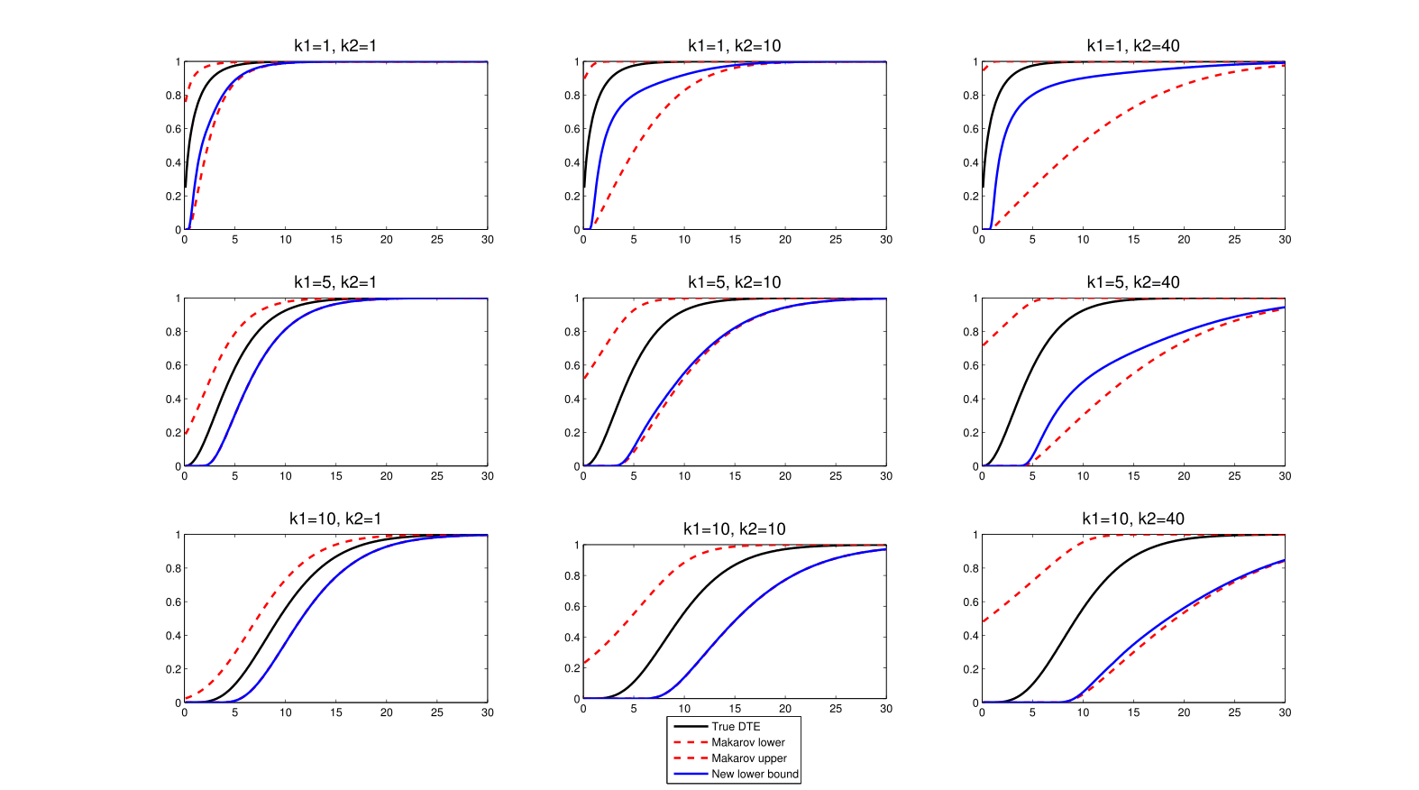
Figure 12: New bounds v.s. Makarov bounds

Figure 12 shows the true DTE as well as Makarov bounds and the improved lower bound under MTR for $k_{1}=1,5,10$ and $k_{2}=1,10,40.$ To see the effect of marginal distributions for the fixed true DTE $\Delta\sim\chi^{2}\left(k_{1}\right),$ I focus on how the DTE bounds change for different values of $k_{2}$ and fixed $k_{1}$.

Figure 12 shows that Makarov bounds and my new lower bound become less informative as $k_{2}$ increases. My data generating process assumes $Y_{1}-Y_{0}\sim\chi^{2}\left(k_{1}\right)$, $Y_{0}\sim N\left(0,k_{2}\right)$ and $Y_{1}-Y_{0}\perp\!\!\!\perp Y_{0}.$  When the true DTE is fixed with a given value of $k_{1},$ both Makarov bounds and my new bounds move further away from the true DTE as the randomness in the potential outcomes $Y_{0}$ and $Y_{1}$ increases with higher $k_{2}$. If $k_{2}=0$ as an extreme case, in which $Y_{0}$ has a degenerate distribution, obviously Makarov bounds as well as my new bounds point-identify the DTE.

Interestingly, as $k_{2}$ increases, my new lower bound moves further away from the true DTE much more slowly than the Makarov lower bound. Therefore, the information gain from MTR, which is represented by the distance between my new lower bound and the Makarov lower bound, increases as $k_{2}$ increases. This shows that under MTR, my new lower bound gets additional information from the larger variation of marginal distributions.

To develop intuition, recall Figure 7(c). Under MTR, the larger variation in marginal distributions $F_{0}$ and $F_{1}$ over the support causes more triangles having positive probability lower bounds, which leads the improvement of my new lower bound. On the other hand, the Makarov lower bound gets no such informational gain because it uses only one triangle while my new lower bound takes advantage of multiple triangles.

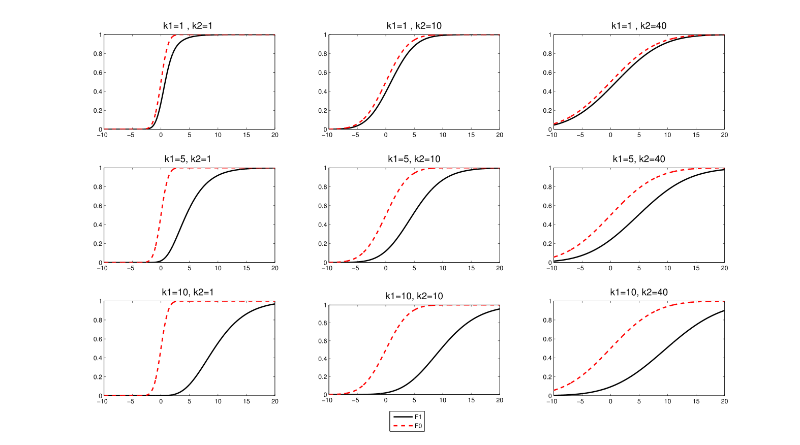
Figure 13: Marginal distributions of potential outcomes

5 Application to the Distribution of Effects of Smoking on Birth Weight

In this section, I apply the results presented in Section 3 to an empirical analysis of the distribution of smoking effects on infant birth weight. Smoking not only has a direct impact on infant birth weight, but is also associated with unobservable factors that affect infant birth weight. I identify marginal distributions of potential infant birth weight with and without smoking by making use of a state cigarette tax hike in Massachusetts (MA) in January 1993 as a source of exogenous variation. I focus on pregnant women who change their smoking behavior from smoking to nonsmoking in response to the tax increase. To identify the distribution of smoking effects, I impose a MTR restriction that smoking has nonpositive effects on infant birth weight with probability one. I propose an estimation procedure and report estimates of the DTE bounds. I compare my new bounds to Makarov bounds to demonstrate the informativeness and usefulness of my methodology.

5.1 Background

Birth weight has been widely used as an indicator of infant health and welfare in economic research. Researchers have investigated social costs associated with low birth weight (LBW), which is defined as birth weight less than 2500 grams, to understand the short term and long term effects of children’s endowments. For example, Almond et al. (2005) estimated the effects of birth weight on medical costs, other health outcomes, and mortality rate, and Currie and Hyson (1999) and Currie and Moretti (2007) evaluated the effects of low birth weight on educational attainment and long term labor market outcomes. Almond and Currie (2011) provide a survey of this literature.

Smoking has been acknowledged as the most significant and preventable cause of LBW, and thus various efforts have been made to reduce the number of women smoking during pregnancy. As one of these efforts, increases in cigarette taxes have been widely used as a policy instrument between 1980 and 2009 in the U. S. Tax rates on cigarettes have increased by approximately $\$0.80$ each year on average across all states, and more than $80$ tax increases of $\$0.25$  have been implemented in the past $15$ years (Simon (2012) and Orzechowski and Walker (2011)).

In the literature, there have been various attempts to clarify the causal effects of smoking on infant birth weight. Most previous empirical studies have evaluated the average effects of smoking or effects on the marginal distribution of potential infant birth weight focusing on the methods to overcome the endogeneity of smoking behavior.

My analysis pays particular attention to the distribution of smoking effects on infant birth weight. The DTE conveys the information on the targets of anti-smoking policy, which is particularly important for this study, because the DTE can answer the following questions: ”how many births are significantly vulnerable to smoking ?” and ”who should the interventions intensively target?”.

I make use of the cigarette tax increase in MA in January of 1993, which increased the state excise tax from $\$0.26$ to $\$0.51$ per pack, as an instrument to identify marginal distributions of potential birth weight acknowledging the presence of endogeneity in smoking behavior. In November 1992, MA voters passed a ballot referendum to raise the tax on tobacco products, and in 1993 the Massachusetts Tobacco Control Program was established with a portion of the funds raised through this referendum. The Massachusetts Tobacco Control Program initiated activities to promote smoking cessation such as media campaigns, smoking cessation counselling, enforcement of local antismoking laws, and educational programs targeted primarily at teenagers and pregnant women.

The IV framework developed by Abadie, Angrist and Imbens (2002) is used to identify and estimate marginal distributions of potential infant birth weight for pregnant women who change their smoking status from smoking to nonsmoking in response to the tax increase. Henceforth, I call this group of people compliers. Based on the estimated marginal distributions, I establish sharp bounds on the smoking effects under the MTR assumption that smoking has adverse effects on infant birth weight.

5.2 Related Literature

The related literature can be divided into three strands by their empirical strategy to overcome the endogenous selection problem. The first strand of the literature, including Almond et al. (2005), assumes that smoking behavior is exogenous conditional on observables such as mother’s and father’s characteristics, prenatal care information, and maternal medical risk factors. However, Caetano (2012) found strong evidence that smoking behavior is still endogenous after controlling for the most complete covariate specification in the literature. The second strand of the literature, including Permutt and Hebel (1989), Evans and Ringel (1999), Lien and Evans (2005), and Hoderlein and Sasaki (2011) takes an IV strategy. Permutt and Hebel (1989) made use of randomized counselling as an exogenous variation, while Evans and Ringel (1999), Hoderlein and Sasaki (2013) took advantage of cigarette tax rates or tax increases. The last strand takes a panel data approach. This approach isolates the effects of unobservables using data on mothers with multiple births and identifies the effect of smoking from the change in their smoking status from one pregnancy to another. To do this, Abrevaya (2006) constructed the panel data set with novel matching algorithms between women having multiple births and children on federal natality data. The panel data set constructed by Abrevaya (2006) has been used in other recent studies such as Arellano and Bonhomme (2011) and Jun et al. (2013). Jun et al. (2013) tested stochastic dominance between two marginal distributions of potential birth weight with and without smoking. Arellano and Bonhomme (2011) identified the distribution of smoking effects using the random coefficient panel data model.

To the best of my knowledge, the only existing study that examines the distribution of smoking effects is Arellano and Bonhomme (2012). While they point-identify the distribution of smoking effects, their approach presumes access to the panel data with individuals who changed their smoking status within their multiple births. Specifically, they use the following panel data model with random coefficients:

$$Y_{it}=\alpha_{i}+\beta_{i}D_{it}+X_{it}^{\prime}\gamma+\varepsilon_{it}$$

where $Y_{it}$ is infant birth weight and $D_{it}$  is an indicator for woman $i$ smoking before she had her $t$-th baby. Extending Kotlarski’s deconvolution idea, they identify the distribution of $\beta_{i}=E\left[Y_{it}|D_{it}=1,\alpha_{i},\beta_{i}\right]-E\left[Y_{it}|D_{it}=0,\alpha_{i},\beta_{i}\right]$, which indicates the distribution of smoking effects in this example. For the identification, they assume strict exogeneity that mothers do not change their smoking behavior from their previous babies’ birth weight. Furthermore, their estimation result is somewhat implausible. It is interpreted that smoking has a positive effect on infant birth weight for approximately 30% mothers. They conjecture that this might result from a misspecification problem such as the strict exogeneity condition, i.i.d. idiosyncratic shock, etc.

Table 1: Data used in the recent literature

	Data	# of obs.
Evans and Ringel (1999)	NCHS (1989-1992)	${10.5}$  million
Almond et al. (2005)	NCHS(1989-1991, PA only)	${491,139}$
Abrevaya (2006)	matched panel constructed from NCHS (1989-1998)	${296,218}$
Arellano and Bonhomme (2011)	matched panel #3 in Abrevaya (2006)	${1,445}$
Jun et al. (2013)	matched panel #3 in Abrevaya (2006)	${2,113}$
Hoderlein and Sasaki (2013)	random sample from NCHS (1989-1999)	${100,000}$

Most existing studies used the Natality Data by the National Center for Health Statistics (NCHS) for its large sample size and a wealth of information on covariates. The birth data is based on birth records from every live birth in the U.S. and contains detailed information on birth outcomes, maternal prenatal behavior and medical status, and demographic attributes. Table 1 describes the data used in the recent literature.

While some studies such as Hoderlein and Sasaki (2011) and Caetano (2012) use the number of cigarettes per day as a continuous treatment variable, most applied research uses a binary variable for smoking. The literature, including Evans and Farrelly (1998), found that individuals, especially women, tend to underreport their cigarette consumption. On the other hand, smoking participation has shown to be more accurately reported among adults in the literature. Moreover, the literature has pointed out that the number of cigarettes may not be a good proxy for the level of nicotine intake. Previous studies, including Chaloupka and Warner (2000), Evans and Farrelly (1998), Farrelly et al. (2004), Adda and Cornaglia (2006), and Abrevaya and Puzzello (2012) discussed that although an increase in cigarette taxes leads to a lower percentage of smokers and less cigarettes consumed by smokers, it causes individuals to purchase cigarettes that contain more tar and nicotine as compensatory behavior.

Although many recent studies are based on the same NCHS data set, their estimates of average smoking effects are quite varied, ranging from -144 grams to -600 grams depending on their estimation methods and samples. Table 2 summarizes their estimates.

Table 2: Estimated average smoking effects on infant birth weight

	Estimate (g)
Evans and Ringel (1999)	-600 $-$ -360
Almond et al. (2005)	-203.2
Abrevaya (2006)	-144 $-$ -178
Arellano and Bonhomme (2011)	-161

5.3 Data

I use the NCHS Natality dataset. My sample consists of births to women who were in their first trimester during the period between two years before and two years after the tax increase. In other words, I consider births to women who conceived babies in MA between October 1990 and September 1994. I define the instrument as an indicator of whether the agent faces the high tax rate from the tax hike during the first trimester of pregnancy. Since the tax increase occurred in MA in January of 1993, the instrument $Z$ can be written as

$$Z=\left\{\begin{array}[c]{cl}1,&\text{if a baby is conceived in Oct. 1992 or later}\\ 0,&\text{if a baby is conceived before Oct. 1992}\end{array}\right.$$ (14)

The first trimester of pregnancy has received particular attention in the medical literature on the effects of smoking. Mainous and Hueston (1994) demonstrated that smokers who quit smoking within the first trimester showed reductions in the proportion of preterm deliveries and low birth weight infants, compared with those who smoked beyond the first trimester. Also, Fingerhut et al. (1990) showed that approximately 70% of women who quit smoking during pregnancy do so as soon as they are aware of their pregnancy, which is mostly the first trimester of pregnancy.

I take only singleton births into account and focus on births to mothers who are white, Hispanic or black, and whose age is between 15 and 44. The covariates that I use to control for observed characteristics include mothers’ race, education, age, martial status, birth year, sex of the baby, the ”Kessner” prenatal care index, pregnancy history, information on various diseases such as anemia, cardiac, diabete alcohol use, etc.

Descriptive statistics for this sample are reported in Table 3. After the tax increase, the smoking rate of pregnant women decreased from 23% to 16%. As expected, babies of nonsmokers are on average heavier than babies of smokers by 214 grams and furthermore, nonsmokers’ infant birth weight stochastically dominate smokers’ infant birth weight as shown in Figure 14. Also, smokers are on average 1.63 years younger, 1.27 years less educated than nonsmokers, and less likely to have adequate prenatal care in the Kessner index. Regarding race, black or Hispanic pregnant women are less likely to smoke than white women.

Table 3: Means and Standard Deviations

		Before/After Tax Increase			Smoking/Nonsmoking
	Entire sample	After	Before	Diff.	Smokers	Nonsmokers	Diff.
# of obs.	297,031	144,251	152,780		57,602	239,429
Smoking	0.19	0.16	0.23	-0.07
(proportion)	[0.40]	[0.36]	[0.42]	(-50.64)
Birth weight	3416.81	3416.73	3416.88	-0.15	3244.31	3458.30	-214.00
(grams)	[556.07]	[556.09]	[556.07]	(-0.07)	[561.28]	[546.75]	(-82.57)
Age	28.51	28.70	28.33	.37	27.19	28.82	-1.63
(years)	[5.70]	[5.75]	[5.65]	(17.58)	[5.67]	[5.66]	(-62.07)
Education	13.46	13.54	13.38	0.15	12.43	13.71	-1.27
	[2.50]	[2.49]	[2.52]	(16.48)	[2.16]	[2.52]	(-112.00)
Married	0.74	0.74	0.75	-0.004	0.58	0.78	-.20
	[0.43]	[0.74]	[.44]	(-2.64)	[.49]	[0.41]	(-90.41)
Black	0.10	0.10	0.10	-0.005	0.07	0.11	-0.03
	[0.30]	[0.29]	[.30]	(-4.22)	[0.26]	[0.31]	(-27.90)
Hispanic	0.10	0.10	0.10	0.002	0.06	0.11	-0.06
	[0.30]	[0.30]	[0.30]	(2.23)	[.24]	[0.32]	(-45.34)
Kessner=1	0.84	.84	0.83	0.01	0.78	0.85	-0.08
	[0.37]	[0.36]	[0.37]	(7.96)	[.42]	[0.35]	(-41.69)
Kessner=2	0.13	0.13	0.14	-0.01	0.18	0.12	0.05
	[0.34]	[0.34]	[0.34]	(-5.75)	[0.38]	[0.33]	(30.35)
Gestation	39.27	39.25	39.29	-0.04	39.14	39.30	-0.17
(weeks)	[2.04]	[2.01]	[2.07]	(-5.88)	[2.24]	[1.99]	(-16.29)

Note: The table reports means and standard deviations (in brackets) for the sample used in this study. The columns showing differences in means (by assignment or treatment status) report the t-statistic (in parentheses) for the null hypothesis of equality in means.

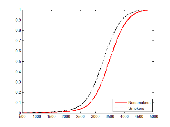
Figure 14: Distribution functions of infant birth weight of smokers and nonsmokers

5.4 Estimation

Using the earlier notation, let $Y$ be observed infant birth weight and $D$ the nonsmoking indicator defined as

$$D=\left\{\begin{tabular}[c]{ll}$1,$&for a nonsmoker\\ $0,$&for a smoker\end{tabular}\right.$$

In addition, let $D_{z}$ denote a potential nonsmoking indicator given $Z=z.$ Let $Y_{0}$ be the potential infant birth weight if the mother is a smoker, while $Y_{1}$ the potential infant birth weight if the mother is not a smoker. As defined in (14), $Z$ is a tax increase indicator during the first trimester. The $k\times 1$ vector $X$ of covariates consists of binary indicators for mother’s race, age, education, marital status, birth order, sex of the baby, ”Kessner” prenatal care index, drinking status, and medical risk factors. Since the treatment variable is nonsmoking here, the estimated effect is the benefit of smoking cessation, which is in turn equal to the absolute value of the adverse effect of smoking. To identify marginal distributions, I impose the standard LATE assumptions following Abadie et al. (2002):

Assumption 2

For almost all values of $X:$

(i) Independence: $\left(Y_{1},Y_{0},D_{1},D_{0}\right)$ is jointly independent of $Z$ given $X$.

(ii) Nontrivial Assignment: $\Pr\left(Z=1|X\right)\in\left(0,1\right).$

(iii) First-stage: $E\left[D_{1}|X\right]\neq E\left[D_{0}|X\right].$

(iv) Monotonicity: $\Pr\left(D_{1}\geq D_{0}|X\right)=1.$

Assumption 2(i) implies that the tax increase exogenously affects the smoking status conditional on observables and that any effect of the tax increase on infant birth weight must be via the change in smoking behavior. This is plausible in my application since the tax increase acts as an exogenous shock. Assumption 2(ii) and (iii) obviously hold in this sample. Assumption 2(iv) is plausible since an increase in cigarette tax rates would never encourage smoking for each individual.

5.4.1 The Marginal Treatment Effect and Local Average Treatment Effect

First, I estimate marginal effects of smoking cessation to see how the mean effect varies with the individual’s tendency to smoke. The marginal treatment effect (MTE) is defined as follows:

$$MTE(x,p)=E[Y_{1}-Y_{0}|X=x,P\left(Z,X\right)=p].$$

where $P\left(Z,X\right)=P(D=1|Z,X),$ which is the probability of not smoking conditional on $Z$ and $X.$ In Heckman and Vytlacil (2005), the MTE is recovered as follows:

$$MTE(x,p)=\frac{\partial}{\partial p}E\left[Y|X=x,P\left(Z,X\right)=p\right].$$

Since the propensity score $p\left(Z,X\right)=\Pr\left(D=1|Z,X\right)$ is unobserved for each agent, I estimate it using the probit specification:

$$p\left(Z,X\right)=\Phi\left(\alpha+\beta Z+X^{\prime}\gamma\right).$$ (15)

Then with the estimated propensity score $\widehat{p}\left(Z,X\right)$ in (15), I estimate the following outcome equation:

$$Y=\mu\left(\widehat{p}\left(Z,X\right),X\right)+u$$ (16)

I estimate the equation (16) using a series approximation. This method is especially convenient to estimate MTE $\frac{\partial\mu}{\partial p}.$ The estimation results for the regressions (15) and (16) are reported in Table C.1 and Table C.2, respectively, in Appendix C. Figure 15 shows estimated marginal treatment effects for each propensity to not smoke. It is observed that the positive effect of smoking cessation on infant birth weight increases as the tendency to smoke increases. That is, the benefit of quitting smoking on child health is larger for women who will still smoke despite facing higher tax rates. In turn, the adverse effect of smoking on infant birth weight is more severe for women with the higher tendency to smoke during pregnancy.

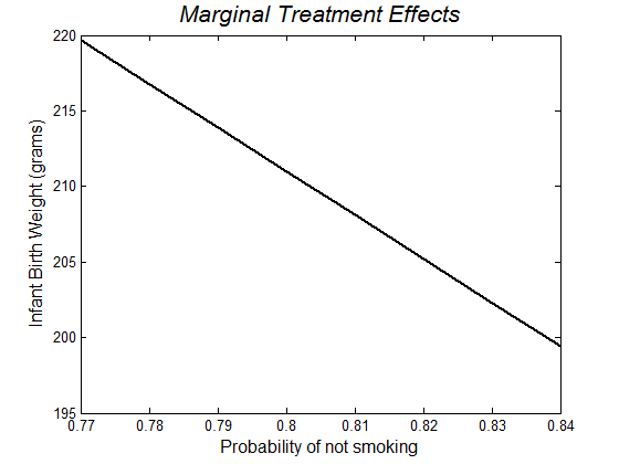
Figure 15: Marginal smoking effects

Next, I estimate LATE from the MTE. The LATE is interpreted as the benefit of smoking cessation for compliers, women who change their smoking status from smoker to nonsmoker in response to the tax increase. It is obtained from marginal treatment effects as follows: for $\overline{p}\left(x\right)=\Pr\left(D=1|Z=1,X=x\right)$ and $\underline{p}=\Pr\left(D=1|Z=0,X=x\right),$

$$E[Y_{1}-Y_{0}|X=x,D_{1}>D_{0}]=\frac{1}{\overline{p}\left(x\right)-\underline{p}\left(x\right)}\int_{\underline{p}\left(x\right)}^{\overline{p}\left(x\right)}MTE(x,p)dp.$$

Table 4 presents estimated LATE for the entire sample and three subgroups of white women, women aged 26-35, and women with some college or college graduates (SCCG). The estimated benefit of smoking cessation is noticeably small for SCCG women, compared to the entire sample and women whose age is between 26 and 35. These MTE and LATE estimates show that births to less educated women or women with a higher tendency to smoke are on average more vulnerable to smoking. The literature, such as Deaton (2003) and Park and Kang (2008), has found a positive association between smoking behavior and other unhealthy lifestyles, and between higher education and a healthier lifestyle. Given this association, my MTE and LATE estimates suggest that births to women with an unhealthier lifestyle on average are more vulnerable to smoking.

Table 4: Local Average Treatment Effects (grams)

Dep. var.: birth weight (grams)	LATE
The entire sample	209
White	133
Age26-35	183
Some college and college graduates (SCCG)	112

5.4.2 Quantile Treatment Effects for Compliers

In this subsection, I estimate the effect of smoking on quantiles of infant birth weight through the quantile treatment effect (QTE) parameter. $q$-QTE measures the difference in the $q$-quantile of $Y_{1}$ and $Y_{0}$, which is written as $Q_{q}\left(Y_{1}\right)-Q_{q}\left(Y_{0}\right)$ where $Q_{q}\left(Y_{d}\right)$ denotes the $q$-quantile of $Y_{d}$ for $d\in\left\{0,1\right\}$.

Lemma 4 forms a basis for causal inferences for compliers under Assumption 2.

Lemma 4 (Abadie et al. (2002))

Given Assumption 2(i),

$$\left(Y_{1},Y_{0}\right)\perp\!\!\!\perp D|X,D_{1}>D_{0}$$

Lemma 4 allows QTE to provide causal interpretations for compliers. Let $Q_{q}\left(Y|X,D,D_{1}>D_{0}\right)$ denote the $q$-quantile of $Y$ given $X$ and $D$ for compliers. Then by Lemma 4,

$$Q_{q}\left(Y|X,D=1,D_{1}>D_{0}\right)-Q_{q}\left(Y|X,D=0,D_{1}>D_{0}\right)$$

represents the causal effect of smoking cessation on the $q$-quantile infant birth weight for compliers. Now I estimate the quantile regression model based on the following specification for the $q$-quantile of $Y$ given $X$ and $D$ for compliers $:$ for $q\in\left(0,1\right),$

$$Q_{q}\left(Y|X,D,D_{1}>D_{0}\right)=\alpha_{q}+\beta_{q}\left(X\right)D+X^{\prime}\gamma_{q},$$ (17)

where $\beta_{q}\left(X\right)=\beta_{1q}+X^{\prime}\beta_{2q}$, $\beta_{q}=\left(\begin{array}[c]{c}\beta_{1q}\\ \beta_{2q}\end{array}\right)$, $\left(\alpha_{q},\beta_{1q}\right)\in\mathbb{R}\times\mathbb{R},$ $\beta_{2q}\in\mathbb{R}^{k}$ and $\gamma_{q}\in\mathbb{R}^{k}$.

I use Abadie et al. (2002)’s estimation procedure. They proposed an estimation method for moments involving $(Y,D,X)$ for compliers by using weighted moments. See Section 3 of Abadie et al. (2002) for details about the estimation procedure and asymptotic distribution of the estimator. Following their estimation strategy, I estimate the equation (17). The estimation results for the equation (17) are documented in Table C.3 in Appendix C.

Smoking is estimated to have significantly negative effects on all quantiles of birth weight. The estimated causal effect of smoking on the $q$-quantile of infant birth weight is $-195$ grams at $q=0.15$, $-214$ grams at $q=0.25$, and $-234$ grams at $q=0.50$. The effect significantly differs by women’s race, education, age, and the quality of prenatal care. This heterogeneity also varies across quantile levels of birth weight. For the low quantiles $q=0.15$ and $0.25$, the adverse effect of smoking is estimated to be the largest for births whose mothers are black and get inadequate prenatal care. In education, the adverse smoking effect is much less severe for college graduates compared to women with other education background. At $q=0.15$, as women’s age increases up to 35 years, the adverse effect of smoking becomes less severe, but it increases with women’s age for births to women who are older than 35 years old.

Controlling for the smoking status, compared to white women, black women bear lighter babies for all quantiles and Hispanic women bear similar weight babies at low quantiles $q=0.15,$ $0.25$ but lighter babies at higher $q>0.5.$ Also, at low quantiles $q=0.15$ and $0.25$, as mothers’ education level increases, the birth weight noticeably increases except for post graduate women. Married women are more likely to give births to heavier babies for low quantiles $q=0.15,$ $0.25,$ $0.50,$ but lighter babies at high quantiles $q=0.75,0.85$. One should be cautious about interpreting the results at high quantiles. At high quantiles, heavier babies do not necessarily mean healthier babies because high birth weight could be also problematic. The prenatal care seems to be associated with birth weight very differently at both ends of quantiles (at $q=0.15$ and at $q=0.85$). At $q=0.15$, women with better prenatal care tend to have lighter babies, while at $q=0.85$ women with better prenatal care are more likely to bear heavier infants. This suggests that women with higher medical risk factors are more likely to have more intense prenatal care.

Table 5: Quantiles of potential outcomes and quantile treatment effects (grams)

(grams)		${\small Q}_{0.15}$	${\small Q}_{0.25}$	${\small Q}_{0.5}$	${\small Q}_{0.75}$	${\small Q}_{0.85}$
Entire Sample	QTE	195	214	234	259	292
	${\small Q}\left(Y_{0}\right)$	2760	2927	3220	3515	3675
	${\small Q}\left(Y_{1}\right)$	2955	3141	3454	3774	3967
White	QTE	204	212	212	227	255
	${\small Q}\left(Y_{0}\right)$	2815	2974	3300	3589	3731
	${\small Q}\left(Y_{1}\right)$	3019	3186	3512	3816	3986
SCCG	QTE	109	165	187	244	194
	${\small Q}\left(Y_{0}\right)$	2908	3031	3316	3566	3798
	${\small Q}\left(Y_{1}\right)$	3017	3196	3503	3810	3992
Age 26-35	QTE	233	180	179	262	283
	${\small Q}\left(Y_{0}\right)$	2781	3008	3331	3557	3720
	${\small Q}\left(Y_{1}\right)$	3014	3188	3510	3818	4003

To estimate marginal distributions of $Y_{0}$ and $Y_{1,}$ I first estimate the model (17) for a fine grid of $q\$with $999$ points from $0.001$ to $0.999$ and obtain quantile curves of $Y_{0}$ and $Y_{1}$ on the fine grid. Note that fitted quantile curves are non-monotonic as shown in Figure 16(a). I sort the estimated values of the quantile curves in an increasing order as proposed by Chernozhukov et al. (2009). They showed that this procedure improves the estimates of quantile functions and distribution functions in finite samples. Figure 16(b) shows the monotonized quantile curves for $Y_{0}$ and $Y_{1}$, respectively. The marginal distribution functions of $Y_{0}$ and $Y_{1}$ are obtained by inverting the monotonized quantile curves.

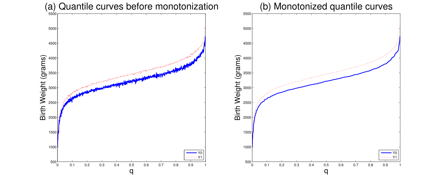
Figure 16: Estimated quantile curves

Table 5 presents estimates of quantiles for potential outcomes and QTE. One noticeable observation is that for SCCG women, low quantiles ($q<0.5$) of birth weight from smokers are remarkably higher compared to those for the entire sample or other subgroups, while their nonsmokers’ birth weight quantiles are similar to those in other groups. This leads to the lower quantile smoking effects for this college education group compared to other groups at low quantiles.

I also obtain the proportion of potential low birth weight infants to smokers and nonsmokers, $F_{0}\left(2,500\right)$ and $F_{1}\left(2,500\right)$, respectively. As shown in Table 6, 6.5% of babies to smokers would have low birth weight, while 4% babies to nonsmokers would have low birth weight. Similar results are obtained for white women and women aged 26-35. A surprising result is obtained for SCCG women. Only 3.5%  of babies to SCCG women who smoke would have low birth weight. This implies that SCCG women who smoke are less likely to have low birth weight infants than women with less education who smoke. One possible explanation for this is that women with higher education are more likely to have healthier lifestyles and this substantially lowers the risk of having low infant birth weight for smoking.

Table 6: The proportion of potential low birth weight infants

(%)	$F_{0}\left(2,500\right)$	$F_{1}\left(2,500\right)$
Entire Sample	6.5	4
White	7	3
SCCG	3.5	2.9
Age 26-35	5.7	3.2

Table 7: The proportion of potential low birth weight infants

(%)	$F_{0}\left(2,500\right)$	$F_{1}\left(2,500\right)$
Entire Sample	6.5	4
White	7	3
SCCG	3.5	2.9
Age 26-35	5.7	3.2

5.4.3 Bounds on the Distribution and Quantiles of Treatment Effects for Compliers

Recall the sharp lower bound under MTR: for $\delta\geq 0,$

$$F_{\Delta}^{L}\left(\delta\right)=\underset{\left\{a_{k}\right\}_{k=-\infty}^{\infty}}{\sup}\sum\limits_{k=-\infty}^{\infty}\max\left\{F_{1}\left(a_{k+1}\right)-F_{0}\left(a_{k}\right),0\right\},$$ (18)

where $0\leq a_{k+1}-a_{k}\leq\delta$ for each integer $k$. To compute the new sharp lower bound from the estimated marginal distribution functions, I plug in the estimates of marginal distribution functions $\widehat{F}_{0}$ and $\ \widehat{F}_{1}$ proposed in the previous subsection. I follow the same computation procedure as in the numerical example of Section 4. I discuss the procedure in Appendix B in detail.

I propose the following plug-in estimators of my new lower bound and Makarov bounds based on the estimators of marginal distributions $\widehat{F}_{0}$ and $\ \widehat{F}_{1}$ proposed in the previous subsection. Note that the infinite sum in the lower bound under MTR in Corollary 1 reduces to the finite sum for the bounded support. For any fixed $\delta>0,$ the consistency of my estimators is immediate.

In Figure 17, I plot my new lower bound and Makarov bounds for the entire sample. One can see substantial identification gains from the distance between my new lower bound and the Makarov lower bound. The most remarkable improvement arises around $q=0.5$ and the refinement gets smaller as $q$ approaches $0$ and $1,$ in turn as $\delta$ approaches $0$ and $2000$. This can be intuitively understood through Figure 7(c). As $\delta$ gets closer to $2000,$ the number of triangles, which is one source of identification gains, decreases to one in the bounded support of each potential outcome. This causes the new lower bound to converge to the Makarov lower bound as $\delta$ approaches $2000$. Also, as $\delta$ converges to $0,$ the identification gain generated by each triangle, which is written as max$\left\{F_{1}(y)-F_{0}(y-\delta),0\right\},$ converges to $0$ under MTR, which implies $F_{1}(y)\leq F_{0}(y)$ for each $y\in\mathbb{R}.$

Figure 17: Bounds on the effect of smoking on birth weight for the entire sample

The quantiles of smoking effects can be obtained by inverting these DTE bounds. Specifically, the upper and lower bounds on the quantile of treatment effects are obtained by inverting the lower bound and upper bound on the DTE, respectively. Note that quantiles of smoking effects show $q$-quantiles of the difference $(Y_{1}-Y_{0})$, while QTE gives the difference between the $q$-quantiles of $Y_{1}$ and those of $Y_{0}$. These two parameters typically have different values. Fan and Park (2009) pointed out that QTE is identical to the quantile of treatment effects under strong conditions. The bounds on the quantile of treatment effects are reported in Table 7 with comparison to QTE, already reported in Table 5. In the entire sample, my new bounds on the quantiles of the treatment effect show $33$% - $45$% refinement for $q=0.15$, $0.25$, $0.5$, $0.75$ compared to Makarov bounds. For the entire sample, my new bounds yield $[0,457]$ grams for the median of the benefit of smoking cessation on infant birth weight, while Makarov bounds yield $[0,843]$ grams. Compared to Makarov bounds, my new bounds are more informative and show that $(457,843]$ should be excluded from the identification region for the median of the effect.

It is worth noting that my new bounds on the quantile of the effects of smoking are much tighter for SCCG women, compared to the entire sample and other subsamples. For $q\leq 0.5$, the refinement rate ranges from 51% to 64% compared to Makarov bounds. For SCCG women, my new sharp bounds on the median are $[0,299]$ grams, while Makarov bounds on the median are $[0,764]$ grams. The higher identification gains result from relatively heavier potential nonsmokers’ infant birth weight, which leads to the shorter distance between two potential outcomes distributions as reported in Table 5. Note that the shorter distance between marginal distributions of potential outcomes improves both my new lower bound and the Makarov lower bound.

Table 7: QTE and bounds on the quantiles of smoking effects

Dep. var.= Birth weight (grams)		${\small Q}_{0.15}$	${\small Q}_{0.25}$	${\small Q}_{0.5}$	${\small Q}_{0.75}$	${\small Q}_{0.85}$
Entire Sample	QTE	195	214	234	259	292
	Makarov	[0,405]	[0,524]	[0,843]	[0,1317]	[80,1634]
	New	[0,265]	[0,304]	[0,457]	[0,882]	[80,1204]
White	QTE	204	212	212	227	255
	Makarov	[0,383]	[0,505]	[0,833]	[0,1274]	[65,1588]
	New	[0,265]	[0,308]	[0,450]	[0,891]	[65,1239]
SCCG	QTE	109	165	187	244	194
	Makarov	[0,311]	[0,428]	[0,764]	[0,1183]	[69,1453]
	New	[0,114]	[0,193]	[0,299]	[0,579]	[69,792]
Age 26-35	QTE	233	180	179	262	283
	Makarov	[0,336]	[0,458]	[0,807]	[0,1324]	[79,1621]
	New	[0,239]	[0,276]	[0,406]	[0,746]	[79,1204]

Although QTE is placed within the identification region for $q=0.15$ to $0.85$ and for all groups, at $q=0.15$, QTE is very close to the upper bound on the quantile of smoking effects for SCCG and age 26-35 subgroups. Furthermore, at $q=0.10$, QTE is placed outside of the improved identification region for SCCG group and age 26-35. This implies that QTE is not identical to the quantile of treatment effects in my example and so one should not interpret the value of QTE as a quantile of smoking effects.

Despite the large improvement of my bounds over Makarov bounds, the difference in the quantiles of the smoking effects between SCCG women and others is still inconclusive from my bounds. The sharp upper bound on the quantile of the effect for the SCCG group is quite lower than that for the entire sample while the sharp lower bound is $0$ for both groups; the identification region for the SCCG group is contained in that for the entire sample. Since the two identification regions overlap, one cannot conclude that the effect at each quantile level $q$ is smaller for the SCCG group. This can be further investigated by developing formal test procedures for the partially identified quantile of treatment effects or by establishing tighter bounds under additional plausible restrictions. I leave these issues for future research.

My empirical analysis shows that smoking is on average more dangerous for infants to women with a higher tendency to smoke. Also, women with SCCG are less likely to have low birth weight babies when they smoke. The estimated bounds on the median of the effect of smoking on infant birth weight are $[-457$,$0]$ grams and $[-299,0]$ grams for the entire sample and for women with SCCG, respectively.

Based on my observations, I suggest that policy makers pay particular attention to smoking women with low education in their antismoking policy design, since these women’s infants are more likely to have low weight. Considering the association between higher education and better personal health care as shown in Park and Kang (2008), it appears that smoking on average does less harm to infants to mothers with a healthier lifestyle. Based on this interpretation, healthy lifestyle campaigns need to be combined with antismoking campaigns to reduce the negative effect of smoking on infant birth weight.

5.5 Testability and Inference on the Bounds

5.5.1 Testability of MTR

My empirical analysis relies on the assumption that smoking of pregnant women has nonpositive effects on infant birth weight with probability one. This MTR assumption is not only plausible but also testable in my setup. While a formal econometric test procedure is beyond the scope of this paper, I briefly discuss testable implications. First, MTR implies stochastic dominance of $Y_{1}$ over $Y_{0}$. Since I point-identify their marginal distributions for compliers, stochastic dominance can be checked from the estimated marginal distribution functions. Except for very low $q$-quantiles with $q<0.006$ where the quantile curves estimates are imprecise as noted in subsection 5.4, my estimated marginal distribution functions satisfy the stochastic dominance for the entire sample and all subgroups. Second, under MTR my new lower bound should be lower than the Makarov upper bound. If MTR is not satisfied, then my new lower bound is not necessarily lower than the Makarov upper bound. In my estimation result, my new lower bound is lower than the Makarov upper bound for all $\delta>0$ and in all subgroups.

5.5.2 Inference and Bias Correction

Asymptotic properties of my estimators other than consistency have not been covered in this paper. The complete asymptotic theory for the estimators can be investigated by adopting arguments from Abadie et al. (2002), Koenker and Xiao (2002), Angrist et al. (2005), and Fan and Park (2010). Abadie et al. (2002) provided asymptotic properties for their weighted quantile regression coefficients for the fixed quantile level $q,$ while Koenker and Xiao (2002) and Angrist et al. (2005) focused on the standard quantile regression $\emph{process}.$ Fan and Park (2010) derived asymptotic properties for the plug-in estimators of Makarov bounds. Since they estimated marginal distribution functions using empirical distributions in the context of randomized experiments, their arguments follow standard empirical process theory. To investigate asymptotic properties of the bounds estimators and the estimated maximizer or minimizer for the bounds, I am currently extending the asymptotic analysis on the quantile regression process presented by Koenker and Xiao (2002) and Angrist et al. (2005) to the quantile curves which are obtained from the weighted quantile regression of Abadie et al. (2002).

Canonical bootstrap procedures may be invalid for inference in this setting. Fan and Park (2010) found that asymptotic distributions of their plug-in estimators for Makarov bounds discontinuously change around the boundary where the true lower and upper Makarov bounds reach zero and one, respectively. Specifically, they estimated the Makarov lower bound $\underset{y}{\sup}\max\left\{F_{1}\left(y\right)-F_{0}\left(y-\delta\right),0\right\}$ using empirical distribution functions $\widehat{F}_{0}$ and $\widehat{F}_{1}$. They found that the asymptotic distribution of their estimator of the Makarov lower bound is discontinuous on the boundary where $\sup_{y}\left\{F_{1}\left(y\right)-F_{0}\left(y-\delta\right)\right\}=0.$ Since my improved lower bound under MTR is written as the supremum of the sum of $\max\left\{F_{1}\left(a_{k}\right)-F_{0}\left(a_{k-1}\right),0\right\}$ over integers $k$, the asymptotic distribution of my plug-in estimator is likely to suffer discontinuities near multiple boundaries where $F_{1}\left(a_{k}\right)-F_{0}\left(a_{k-1}\right)=0$ for each integer $k$. To avoid the failure of the standard bootstrap, I recommend subsampling or the fewer than $n$ bootstrap procedure following Politis et al. (1999), Andrews (2000), Andrews and Han (2009).

Although the estimator $\widehat{F}_{\Delta}^{NL}$ is consistent, it may have a nonnegligible bias in small samples. I suggest that one use a bias-adjusted estimator based on subsampling when the sample size is small in practice. Let

$$\widehat{F}_{\Delta,n,b,j}^{NL}\left(\delta\right)=\underset{0\leq y\leq\delta}{\sup}\sum_{k=\left\lfloor\frac{500-y}{\delta}\right\rfloor}^{\left\lfloor\frac{5500-y}{\delta}\right\rfloor+1}\max\left(\widehat{F}_{1}^{n,b,j}\left(y+k\delta\right)-\widehat{F}_{0}^{n,b,j}\left(y+\left(k-1\right)\delta\right),0\right),$$

where for $d=0,1,$ $\widehat{F}_{d}^{n,b,j}$ is an estimator of $F_{d}$ from the $j$th subsample $\{\left(Y_{j_{1}},D_{j_{1}}\right),...,\left(Y_{j_{b}},D_{j_{b}}\right)\}$ with the subsample size $b$ out of $n$ observations s.t. $j_{1}\neq$ $j_{2}\neq\ldots\neq j_{b},$ $b<n$ and $j=1,...,\left(\begin{array}[c]{c}n\\ b\end{array}\right)$. Then the subsampling bias-adjusted estimator $\widetilde{F}_{\Delta}^{NL}\left(\delta\right)$ is

$$\widetilde{F}_{\Delta}^{NL}\left(\delta\right) =\widehat{F}_{\Delta}^{NL}\left(\delta\right)-\frac{1}{q_{n}}\sum\limits_{j=1}^{q_{n}}\left\{\widehat{F}_{\Delta,n,b,j}^{NL}\left(\delta\right)-\widehat{F}_{\Delta}^{NL}\left(\delta\right)\right\}$$

$$=2\widehat{F}_{\Delta}^{NL}\left(\delta\right)-\frac{1}{q_{n}}\sum\limits_{j=1}^{q_{n}}\widehat{F}_{\Delta,n,b,j}^{NL}\left(\delta\right),$$

where $q_{n}=\left(\begin{array}[c]{c}n\\ b\end{array}\right).$

6 Conclusion

In this paper, I have proposed a novel approach to identifying the DTE under general support restrictions on the potential outcomes. My approach involves formulating the problem as an optimal transportation linear program and embedding support restrictions into the cost function with an infinite Lagrange multiplier by taking advantage of their linearity in the entire joint distribution. I have developed the dual formulation for $\{0,1,\infty\}$-valued costs to overcome the technical challenges associated with optimization over the space of joint distributions. This contrasts sharply with the existing copula approach, which requires one to find out the joint distributions achieving sharp bounds given restrictions.

I have characterized the identification region under general support restrictions and derived sharp bounds on the DTE for economic examples. My identification result has been applied to the empirical analysis of the distribution of smoking effects on infant birth weight. I have proposed an estimation procedure for the bounds. The empirical results have shown that MTR has a substantial power to identify the distribution of smoking effects when the marginal distributions of the potential outcomes are given.

In some cases, information concerning the relationship between potential outcomes cannot be represented by support restrictions. Moreover, it is also sometimes the case that the joint distribution function itself is of interest. In a companion paper, I propose a method to identify the DTE and the joint distribution when weak stochastic dependence restrictions among unobservables are imposed in triangular systems, which consist of an outcome equation and a selection equation.

Appendix A

In Appendix A. I provide technical proofs for Theorem 1, Corollary 1 and Corollary 2. Throughout Appendix A, the function $\varphi$ is assumed to be bounded and continuous without loss of generality by Lemma 2.

Proof of Theorem 1

Since the proofs of characterization of $F_{\Delta}^{U}$ and $F_{\Delta}^{L}$ are very similar, I provide a proof for characterization of $F_{\Delta}^{L}$ only. Let

$$I\left[\pi\right] =\int\left\{\boldsymbol{1}\left\{y_{1}-y_{0}<\delta\right\}+\lambda\left(1-\boldsymbol{1}_{C}\left(y_{0},y_{1}\right)\right)\right\}d\pi,$$

$$J\left(\varphi,\psi\right) =\int\varphi d\mu_{0}+\int\psi d\mu_{1},$$

for $\lambda=\infty.$ To prove Theorem 1, I introduce Lemma A.1:

Lemma A.1

For any function $f:\mathbb{R}\rightarrow\mathbb{R},$ $s\in[0,1],$ and nonnegative integer $k,$ define $A_{k}^{+}$ and $A_{k}^{-}$ to be level sets of a function $f$ as follows:

$$A_{k}^{+}\left(f,s\right) =\left\{y\in\mathbb{R};f(y)>s+k\right\},$$

$$A_{k}^{-}\left(f,s\right) =\left\{y\in\mathbb{R};f(y)\leq-\left(s+k\right)\right\}.$$

Then for the following dual problems

$$\underset{\pi\in\Pi\left(\mu_{0},\mu_{1}\right)}{\inf}I\left[\pi\right]=\underset{\left(\varphi,\psi\right)\in\Phi_{c}}{\sup}J\left(\varphi,\psi\right),$$

each $\left(\varphi,\psi\right)\in\Phi_{c}$ can be represented as a continuous convex combination of a continuum of pairs of the form

$$\left(\sum\limits_{k=0}^{\infty}\boldsymbol{1}_{A_{k}^{+}\left(\varphi,s\right)}-\sum\limits_{k=0}^{\infty}\boldsymbol{1}_{A_{k}^{-}\left(\varphi,s\right)},\sum\limits_{k=0}^{\infty}\boldsymbol{1}_{A_{k}^{+}\left(\psi,s\right)}-\sum\limits_{k=0}^{\infty}\boldsymbol{1}_{A_{k}^{-}\left(\psi,s\right)}\right)\in\Phi_{c}$$

Proof of Lemma A.1

By Lemma 2,

$$\underset{\pi\in\Pi\left(\mu_{0},\mu_{1}\right)}{\inf}I\left[\pi\right]=\underset{\left(\varphi,\psi\right)\in\Phi_{c}}{\sup}J\left(\varphi,\psi\right),$$

where $\Phi_{c}$ is the set of all pairs $\left(\varphi,\psi\right)$ in $L^{1}\left(dF_{0}\right)$ $\times L^{1}\left(dF_{1}\right)$ such that

$$\varphi\left(y_{0}\right)+\psi\left(y_{1}\right)\leq\boldsymbol{1}\left\{y_{1}-y_{0}<\delta\right\}+\lambda\left(1-\boldsymbol{1}_{C}\left(y_{0},y_{1}\right)\right)\text{ for all }\left(y_{0},y_{1}\right).$$ (A.1)

Note that $\Phi_{c}$ is a convex set. From the definition of $A_{k}^{+}\left(f,s\right)$ and $A_{k}^{-}\left(f,s\right),$ for any function $f:\mathbb{R}\rightarrow\mathbb{R}$ and $s\in(0,1],$

$$\ldots\subseteq A_{1}^{+}\left(f,s\right)\subseteq A_{0}^{+}\left(f,s\right)\subseteq\left(A_{0}^{-}\left(f,s\right)\right)^{c}\subseteq\left(A_{1}^{-}\left(f,s\right)\right)^{c}\subseteq\ldots.,$$ (A.2)

as illustrated in Figure A.1.

$$\text{Figure A.1: Monotonicity of }\left\{A_{k}^{+}\left(f,s\right)\right\}_{k=0}^{\infty}\text{ and }\left\{A_{k}^{-}\left(f,s\right)\right\}_{k=0}^{\infty}$$

Let

$$\varphi_{+}\left(x\right) =\max\left\{\varphi(x),0\right\}\geq 0,$$

$$\varphi_{-}\left(x\right) =\min\left\{\varphi(x),0\right\}\leq 0.$$

By the layer cake representation theorem, $\varphi_{+}\left(x\right)$ can be written as

$$\varphi_{+}\left(x\right) =\int_{0}^{\varphi_{+}\left(x\right)}ds$$ (A.3)

$$=\int_{0}^{\infty}\boldsymbol{1}\left\{\varphi_{+}\left(x\right)>s\right\}ds$$

$$=\sum_{k=0}^{\infty}\int_{0}^{1}\boldsymbol{1}\left\{\varphi_{+}\left(x\right)>s+k\right\}ds$$

$$=\int_{0}^{1}\sum_{k=0}^{\infty}\boldsymbol{1}\left\{\varphi_{+}\left(x\right)>s+k\right\}ds$$

$$=\int_{0}^{1}\sum_{k=0}^{\infty}\boldsymbol{1}\left\{\varphi\left(x\right)>s+k\right\}ds$$

$$=\int_{0}^{1}\sum_{k=0}^{\infty}\boldsymbol{1}_{A_{k}^{+}\left(\varphi,s\right)}\left(x\right)ds,$$

where $A_{k}^{+}\left(f,s\right)=\left\{y\in\mathbb{R};f(y)>s+k\right\}$ for any function $f.$ The fourth equality in (A.3) follows from Fubini’s theorem. Similarly, the nonpositive function $\varphi_{-}\left(x\right)$ can be represented as

$$\varphi_{-}\left(x\right) =-\int_{0}^{\infty}\boldsymbol{1}\left\{\varphi_{-}\left(x\right)\leq-s\right\}ds$$

$$=-\sum_{k=0}^{\infty}\int_{0}^{1}\boldsymbol{1}\left\{\varphi_{-}\left(x\right)\leq-\left(s+k\right)\right\}ds$$

$$=-\int_{0}^{1}\sum_{k=0}^{\infty}\boldsymbol{1}\left\{\varphi_{-}\left(x\right)\leq-\left(s+k\right)\right\}ds$$

$$=-\int_{0}^{1}\sum_{k=0}^{\infty}\boldsymbol{1}\left\{\varphi\left(x\right)\leq-\left(s+k\right)\right\}ds$$

$$=-\int_{0}^{1}\sum_{k=0}^{\infty}\boldsymbol{1}_{A_{k}^{-}\left(\varphi,s\right)}\left(x\right)ds.$$

where $A_{k}^{-}\left(f,s\right)=\left\{y\in\mathbb{R};f(y)\leq-\left(s+k\right)\right\}$ for any function $f.$ Similarly, $\psi_{+}\left(x\right)$ and $\psi_{-}\left(x\right)$ are written as follows:

$$\psi_{+}\left(x\right) =\int_{0}^{1}\sum_{k=0}^{\infty}\boldsymbol{1}_{A_{k}^{+}\left(\psi,s\right)}\left(x\right)ds,$$

$$\psi_{-}\left(x\right) =-\int_{0}^{1}\sum_{k=0}^{\infty}\boldsymbol{1}_{A_{k}^{-}\left(\psi,s\right)}\left(x\right)ds.$$

For any $\left(\varphi,\psi\right)\in$ $\Phi_{c},$ one can write

$$\left(\varphi,\psi\right)$$

$$=\left(\varphi_{+}+\varphi_{-},\psi_{+}+\psi_{-}\right)$$

$$=\int_{0}^{1}\left(\sum_{k=0}^{\infty}\left(\boldsymbol{1}_{A_{k}^{+}\left(\varphi,s\right)}-\boldsymbol{1}_{A_{k}^{-}\left(\varphi,s\right)}\right)ds,\sum_{k=0}^{\infty}\left(\boldsymbol{1}_{A_{k}^{+}\left(\psi,s\right)}-\boldsymbol{1}_{A_{k}^{-}\left(\psi,s\right)}\right)\right)ds,$$

which is a continuous convex combination of a continuum of pairs of

$$\left(\sum_{k=0}^{\infty}\left(\boldsymbol{1}_{A_{k}^{+}\left(\varphi,s\right)}-\boldsymbol{1}_{A_{k}^{-}\left(\varphi,s\right)}\right),\sum_{k=0}^{\infty}\left(\boldsymbol{1}_{A_{k}^{+}\left(\psi,s\right)}-\boldsymbol{1}_{A_{k}^{-}\left(\psi,s\right)}\right)\right)_{s\in[0,1]}.$$

To see if $\left(\sum_{k=0}^{\infty}\left(\boldsymbol{1}_{A_{k}^{+}d\left(\varphi,s\right)}-\boldsymbol{1}_{A_{k}^{-}\left(\varphi,s\right)}\right),\sum_{k=0}^{\infty}\left(\boldsymbol{1}_{A_{k}^{+}\left(\psi,s\right)}-\boldsymbol{1}_{A_{k}^{-}\left(\psi,s\right)}\right)\right)\in\Phi_{c},$ check the following: for any $s\in[0,1]$ and $\lambda=\infty,$

$$\sum_{k=0}^{\infty}\left(\boldsymbol{1}_{A_{k}^{+}\left(\varphi,s\right)}\left(y_{0}\right)-\boldsymbol{1}_{A_{k}^{-}\left(\varphi,s\right)}\left(y_{0}\right)\right)+\sum_{k=0}^{\infty}\left(\boldsymbol{1}_{A_{k}^{+}\left(\psi,s\right)}\left(y_{1}\right)-\boldsymbol{1}_{A_{k}^{-}\left(\psi,s\right)}\left(y_{1}\right)\right)$$ (A.4)

$$\leq\boldsymbol{1}\left\{y_{1}-y_{0}<\delta\right\}+\lambda\left(1-\boldsymbol{1}_{C}\left(y_{0},y_{1}\right)\right)\text{.}$$

The nontrivial case to check is when the LHS in (A.4)  is positive. Consider the case where $s+t<\varphi\left(y_{0}\right)\leq s+t+1$ and $-\left(s+t\right)<\psi\left(y_{1}\right)\leq-\left(s+t-1\right)$ for some nonnegative integer $t$ and $s\in[0,1]$. Then,

$$\sum_{k=0}^{\infty}\left(\boldsymbol{1}_{A_{k}^{+}\left(\varphi,s\right)}\left(y_{0}\right)-\boldsymbol{1}_{A_{k}^{-}\left(\varphi,s\right)}\left(y_{0}\right)\right) =t+1,$$

$$\sum_{k=0}^{\infty}\left(\boldsymbol{1}_{A_{k}^{+}\left(\psi,s\right)}\left(y_{1}\right)-\boldsymbol{1}_{A_{k}^{-}\left(\psi,s\right)}\left(y_{1}\right)\right) =-t,$$

and so the LHS in (A.4) is $1$. Also, it follows from (A.1) that for $\left(y_{0},y_{1}\right)\in\mathbb{R}\times$ $\mathbb{R}$ s.t. $s+t\leq\varphi\left(y_{0}\right)<s+t+1$ and $-\left(s+t\right)<\psi\left(y_{1}\right),$

$$0<\varphi\left(y_{0}\right)+\psi\left(y_{1}\right)\leq\boldsymbol{1}\left\{y_{1}-y_{0}<\delta\right\}+\lambda\left(1-\boldsymbol{1}_{C}\left(y_{0},y_{1}\right)\right),$$

and thus (A.4) is satisfied in this case from the following:

$$\boldsymbol{1}\left\{y_{1}-y_{0}<\delta\right\}+\lambda\left(1-\boldsymbol{1}_{C}\left(y_{0},y_{1}\right)\right)\geq 1.$$

Consider another case where $s+t\leq\varphi\left(y_{0}\right)<s+t+1$ and $-\left(s+t-1\right)<\psi\left(y_{1}\right)\leq-\left(s+t-2\right)$ for some nonnegative integer $t$ and $s\in[0,1]$. Then the LHS in (A.4) is $2.$ Moreover, since $\varphi\left(y_{0}\right)+\psi\left(y_{1}\right)>1$, for $\left(y_{0},y_{1}\right)\in\mathbb{R}\times$ $\mathbb{R}$ s.t. $s+t\leq\varphi\left(y_{0}\right)<s+t+1$ and $-\left(s+t-1\right)<\psi\left(y_{1}\right),$ by (A.1)

$$1<\varphi\left(y_{0}\right)+\psi\left(y_{1}\right)\leq\boldsymbol{1}\left\{y_{1}-y_{0}<\delta\right\}+\lambda\left(1-\boldsymbol{1}_{C}\left(y_{0},y_{1}\right)\right),$$

and thus (A.4) is also satisfied from the following:

$$\boldsymbol{1}\left\{y_{1}-y_{0}<\delta\right\}+\lambda\left(1-\boldsymbol{1}_{C}\left(y_{0},y_{1}\right)\right)=\infty.$$

Similarly, it can be proven that (A.4) is also satisfied for other nontrivial cases. Therefore it concludes that each $\left(\varphi,\psi\right)\in\Phi_{c}$ can be written as a continuous convex combination of a continuum of pairs of the form

$$\left(\sum\limits_{k=0}^{\infty}\left(\boldsymbol{1}_{A_{k}^{+}\left(\varphi,s\right)}-\boldsymbol{1}_{A_{k}^{-}\left(\varphi,s\right)}\right),\sum\limits_{k=0}^{\infty}\left(\boldsymbol{1}_{A_{k}^{+}\left(\psi,s\right)}-\boldsymbol{1}_{A_{k}^{-}\left(\psi,s\right)}\right)\right).$$

${\small\blacksquare}$

Proof of Theorem 1

By Lemma A.1, $\left(\varphi,\psi\right)\in$ $\Phi_{c}$ can be represented as a continuous convex combination of a continuum of pairs of the form

$$\left(\sum\limits_{k=0}^{\infty}\left(\boldsymbol{1}_{A_{k}^{+}\left(\varphi,s\right)}-\boldsymbol{1}_{A_{k}^{-}\left(\varphi,s\right)}\right),\sum\limits_{k=0}^{\infty}\left(\boldsymbol{1}_{A_{k}^{+}\left(\psi,s\right)}-\boldsymbol{1}_{A_{k}^{-}\left(\psi,s\right)}\right)\right),$$

with

$$\text{ }\sum\limits_{k=0}^{\infty}\left(\boldsymbol{1}_{A_{k}^{+}\left(\varphi,s\right)}\left(y_{0}\right)-\boldsymbol{1}_{A_{k}^{-}\left(\varphi,s\right)}\left(y_{0}\right)\right)+\sum\limits_{k=0}^{\infty}\left(\boldsymbol{1}_{A_{k}^{+}\left(\psi,s\right)}\left(y_{1}\right)-\boldsymbol{1}_{A_{k}^{-}\left(\psi,s\right)}\left(y_{1}\right)\right)$$

$$\leq\boldsymbol{1}\left\{y_{1}-y_{0}<\delta\right\}+\lambda\left(1-\boldsymbol{1}_{C}\left(y_{0},y_{1}\right)\right).$$

Since $\Phi_{c}$ is a convex set and $J\left(\varphi,\psi\right)=\int\varphi dF_{0}+\int\psi dF_{1}$ is a linear functional, for all $\left(\varphi,\psi\right)\in$ $\Phi_{c}$, there exists $s\in(0,1]$ such that

$$J\left(\sum\limits_{k=0}^{\infty}\left(\boldsymbol{1}_{A_{k}^{+}\left(\varphi,s\right)}-\boldsymbol{1}_{A_{k}^{-}\left(\varphi,s\right)}\right),\sum\limits_{k=0}^{\infty}\left(\boldsymbol{1}_{A_{k}^{+}\left(\psi,s\right)}-\boldsymbol{1}_{A_{k}^{-}\left(\psi,s\right)}\right)\right)\geq J\left(\varphi,\psi\right).$$ (A.5)

Thus, the value of $\underset{\left(\varphi,\psi\right)\in\Phi_{c}}{\sup}J\left(\varphi,\psi\right)$ is unchanged even if one restricts the supremum to pairs of the form $\left(\sum\limits_{k=0}^{\infty}\left(\boldsymbol{1}_{A_{k}^{+}\left(\varphi,s\right)}-\boldsymbol{1}_{A_{k}^{-}\left(\varphi,s\right)}\right),\sum\limits_{k=0}^{\infty}\left(\boldsymbol{1}_{A_{k}^{+}\left(\psi,s\right)}-\boldsymbol{1}_{A_{k}^{-}\left(\psi,s\right)}\right)\right).$ Hence for all $\left(y_{0},y_{1}\right)\in\mathbb{R}^{2}$,

$$\sum\limits_{k=0}^{\infty}\left(\boldsymbol{1}_{A_{k}^{+}\left(\varphi,s\right)}\left(y_{0}\right)-\boldsymbol{1}_{A_{k}^{-}\left(\varphi,s\right)}\left(y_{0}\right)\right)+\sum\limits_{k=0}^{\infty}\left(\boldsymbol{1}_{A_{k}^{+}\left(\psi,s\right)}\left(y_{1}\right)-\boldsymbol{1}_{A_{k}^{-}\left(\psi,s\right)}\left(y_{1}\right)\right)$$

$$\leq\boldsymbol{1}\left\{y_{1}-y_{0}<\delta\right\}+\lambda\left(1-\boldsymbol{1}_{C}\left(y_{0},y_{1}\right)\right),$$

which implies that for each $y_{1}\in\mathbb{R},$

$$-\infty <\underset{y_{0}\in\mathbb{R}}{\sup}\left[\sum\limits_{k=0}^{\infty}\left(\boldsymbol{1}_{A_{k}^{+}\left(\varphi,s\right)}\left(y_{0}\right)-\boldsymbol{1}_{A_{k}^{-}\left(\varphi,s\right)}\left(y_{0}\right)\right)-\boldsymbol{1}\left(y_{1}-y_{0}<\delta\right)-\lambda\left(1-\boldsymbol{1}_{C}\left(y_{0},y_{1}\right)\right)\right]$$

$$\leq-\sum\limits_{k=0}^{\infty}\left(\boldsymbol{1}_{A_{k}^{+}\left(\psi,s\right)}\left(y_{1}\right)-\boldsymbol{1}_{A_{k}^{-}\left(\psi,s\right)}\left(y_{1}\right)\right).$$

Define $\left\{A_{k,D}^{+}\left(\varphi,s\right)\right\}_{k=0}^{\infty},$ $\left\{A_{k,D}^{-}\left(\varphi,s\right)\right\}_{k=0}^{\infty}$ as follows:

$$A_{k,D}^{+}\left(\varphi,s\right) =\begin{tabular}[c]{l}$\left\{y_{1}\in\mathbb{R}|\exists y_{0}\in A_{k}^{+}\left(\varphi,s\right)\text{ s.t. }y_{1}-y_{0}\geq\delta\text{ and }\left(y_{0},y_{1}\right)\in C\right\}$\\ $\cup\left\{y_{1}\in\mathbb{R}|\exists y_{0}\in A_{k+1}^{+}\left(\varphi,s\right)\text{ s.t. }y_{1}-y_{0}<\delta\text{ and }\left(y_{0},y_{1}\right)\in C\right\}$\\ $\text{for any integer }k\geq 0,$\end{tabular}$$ (A.9)

$$A_{0,D}^{-}\left(\varphi,s\right) =\begin{tabular}[c]{l}$\left\{y_{1}\in\mathbb{R}|\forall y_{0}\leq y_{1}-\delta\text{ s.t. }\left(y_{0},y_{1}\right)\in C,\text{ }y_{0}\in A_{0}^{-}\left(\varphi,s\right)\right\}$\\ $\cap\left\{y_{1}\in\mathbb{R}|\forall y_{0}>y_{1}-\delta\text{ s.t. }\left(y_{0},y_{1}\right)\in C,\text{ }y_{0}\in\left(A_{0}^{+}\left(\varphi,s\right)\right)^{c}\right\},$\end{tabular}$$ (A.12)

$$A_{k,D}^{-}\left(\varphi,s\right) =\begin{tabular}[c]{l}$\left\{y_{1}\in\mathbb{R}|\forall y_{0}\leq y_{1}-\delta\text{ s.t. }\left(y_{0},y_{1}\right)\in C,\text{ }y_{0}\in A_{k}^{-}\left(\varphi,s\right)\right\}$\\ $\cap\left\{y_{1}\in\mathbb{R}|\forall y_{0}>y_{1}-\delta\text{ s.t. }\left(y_{0},y_{1}\right)\in C,\text{ }y_{0}\in A_{k-1}^{-}\left(\varphi,s\right)\right\}\text{ }$\\ $\text{for any integer }k>0.$\end{tabular}$$ (A.16)

Also, according to the definitions above and Figure A.1, if $y_{1}\in A_{\rho,D}^{+}\left(\varphi,s\right)$ for some $\rho\geq 0,$ then

$$\underset{y_{0}\in\mathbb{R}}{\sup}\left[\sum\limits_{k=0}^{\infty}\left(\boldsymbol{1}_{A_{k}^{+}\left(\varphi,s\right)}\left(y_{0}\right)-\boldsymbol{1}_{A_{k}^{-}\left(\varphi,s\right)}\left(y_{0}\right)\right)-\boldsymbol{1}\left\{y_{1}-y_{0}<\delta\right\}-\lambda\left(1-\boldsymbol{1}_{C}\left(y_{0},y_{1}\right)\right)\right]$$

$$\geq\rho+1,$$

and if $y_{1}\in A_{\rho,D}^{-}\left(\varphi,s\right)$  for some $\rho\geq 0,$

$$\underset{y_{0}\in\mathbb{R}}{\sup}\left[\sum\limits_{k=0}^{\infty}\left(\boldsymbol{1}_{A_{k}^{+}\left(\varphi,s\right)}\left(y_{0}\right)-\boldsymbol{1}_{A_{k}^{-}\left(\varphi,s\right)}\left(y_{0}\right)\right)-\boldsymbol{1}\left\{y_{1}-y_{0}<\delta\right\}-\lambda\left(1-\boldsymbol{1}_{C}\left(y_{0},y_{1}\right)\right)\right]$$

$$\leq-\left(\rho+1\right).$$

Hence, if $y_{1}\in A_{\rho,D}^{+}\left(\varphi,s\right)-A_{\rho+1,D}^{+}\left(\varphi,s\right),$ then

$$\underset{y_{0}\in\mathbb{R}}{\sup}\left[\sum\limits_{k=0}^{\infty}\left(\boldsymbol{1}_{A_{k}^{+}\left(\varphi,s\right)}\left(y_{0}\right)-\boldsymbol{1}_{A_{k}^{-}\left(\varphi,s\right)}\left(y_{0}\right)\right)-\boldsymbol{1}\left\{y_{1}-y_{0}<\delta\right\}-\lambda\left(1-\boldsymbol{1}_{C}\left(y_{0},y_{1}\right)\right)\right]$$

$$=\rho+1,$$

and if $y_{1}\in A_{\rho,D}^{-}\left(\varphi,s\right)-A_{\rho+1,D}^{-}\left(\varphi,s\right),$ then

$$\underset{y_{0}\in\mathbb{R}}{\sup}\left[\sum\limits_{k=0}^{\infty}\left(\boldsymbol{1}_{A_{k}^{+}\left(\varphi,s\right)}\left(y_{0}\right)-\boldsymbol{1}_{A_{k}^{-}\left(\varphi,s\right)}\left(y_{0}\right)\right)-\boldsymbol{1}\left\{y_{1}-y_{0}<\delta\right\}-\lambda\left(1-\boldsymbol{1}_{C}\left(y_{0},y_{1}\right)\right)\right]$$

$$=-\left(\rho+1\right).$$

Hence,

$$\sum\limits_{k=0}^{\infty}\left(\boldsymbol{1}_{A_{k,D}^{+}\left(\varphi,s\right)}\left(y_{1}\right)-\boldsymbol{1}_{A_{k,D}^{-}\left(\varphi,s\right)}\left(y_{1}\right)\right)$$

$$=\underset{y_{0}\in\mathbb{R}}{\sup}\left[\sum\limits_{k=0}^{\infty}\left(\boldsymbol{1}_{A_{k}^{+}\left(\varphi,s\right)}\left(y_{0}\right)-\boldsymbol{1}_{A_{k}^{-}\left(\varphi,s\right)}\left(y_{0}\right)\right)-\boldsymbol{1}\left\{y_{1}-y_{0}<\delta\right\}-\lambda\left(1-\boldsymbol{1}_{C}\left(y_{0},y_{1}\right)\right)\right]$$

$$\leq-\sum\limits_{k=0}^{\infty}\left(\boldsymbol{1}_{A_{k}^{+}\left(\psi,s\right)}\left(y_{1}\right)-\boldsymbol{1}_{A_{k}^{-}\left(\psi,s\right)}\left(y_{1}\right)\right).$$

Now define

$$A_{k}\left(\varphi,s\right) =\left\{\begin{tabular}[c]{ll}$A_{k}^{+}\left(\varphi,s\right),$&if $k\geq 0,$\\ $\left(A_{-k-1}^{-}\left(\varphi,s\right)\right)^{c},$&if $k<0,$\end{tabular}\right.$$

$$A_{k}^{D}\left(\varphi,s\right) =\left\{\begin{tabular}[c]{ll}$A_{k,D}^{+}\left(\varphi,s\right),$&if $k\geq 0,$\\ $\left(A_{-k-1,D}^{-}\left(\varphi,s\right)\right)^{c},$&if $k<0.$\end{tabular}\right.$$

Then for all $\left(y_{0},y_{1}\right)\in\mathbb{R}^{2},$

$$\boldsymbol{1}\left\{y_{1}-y_{0}<\delta\right\}+\lambda\left(1-\boldsymbol{1}_{C}\left(y_{0},y_{1}\right)\right)$$ (A.17)

$$\geq\sum\limits_{k=0}^{\infty}\left(\boldsymbol{1}_{A_{k}^{+}\left(\varphi,s\right)}\left(y_{0}\right)-\boldsymbol{1}_{A_{k}^{-}\left(\varphi,s\right)}\left(y_{0}\right)\right)-\sum\limits_{k=0}^{\infty}\left(\boldsymbol{1}_{A_{k,D}^{+}\left(\varphi,s\right)}\left(y_{1}\right)-\boldsymbol{1}_{A_{k,D}^{-}\left(\varphi,s\right)}\left(y_{1}\right)\right)$$

$$=\sum\limits_{k=0}^{\infty}\left\{\left(\boldsymbol{1}_{A_{k}^{+}\left(\varphi,s\right)}\left(y_{0}\right)-\boldsymbol{1}_{A_{k}^{-}\left(\varphi,s\right)}\left(y_{0}\right)\right)-\left(\boldsymbol{1}_{A_{k,D}^{+}\left(\varphi,s\right)}\left(y_{1}\right)-\boldsymbol{1}_{A_{k,D}^{-}\left(\varphi,s\right)}\left(y_{1}\right)\right)\right\}$$

$$=\sum\limits_{k=0}^{\infty}\left\{\boldsymbol{1}_{A_{k}^{+}\left(\varphi,s\right)}\left(y_{0}\right)+\left(1-\boldsymbol{1}_{A_{k}^{-}\left(\varphi,s\right)}\left(y_{0}\right)\right)-\boldsymbol{1}_{A_{k,D}^{+}\left(\varphi,s\right)}\left(y_{1}\right)-\left(1-\boldsymbol{1}_{A_{k,D}^{-}\left(\varphi,s\right)}\left(y_{1}\right)\right)\right\}$$

$$=\sum\limits_{k=0}^{\infty}\left\{\left(\boldsymbol{1}_{A_{k}^{+}\left(\varphi,s\right)}\left(y_{0}\right)+\boldsymbol{1}_{\left(A_{k}^{-}\left(\varphi,s\right)\right)^{c}}\left(y_{0}\right)\right)-\left(\boldsymbol{1}_{A_{k,D}^{+}\left(\varphi,s\right)}\left(y_{1}\right)+\boldsymbol{1}_{\left(A_{k,D}^{-}\left(\varphi,s\right)\right)^{c}}\left(y_{1}\right)\right)\right\}$$

$$=\sum\limits_{k=0}^{\infty}\left(\boldsymbol{1}_{A_{k}^{+}\left(\varphi,s\right)}\left(y_{0}\right)-\boldsymbol{1}_{A_{k,D}^{+}\left(\varphi,s\right)}\left(y_{1}\right)\right)+\sum\limits_{k=0}^{\infty}\left(\boldsymbol{1}_{\left(A_{k}^{-}\left(\varphi,s\right)\right)^{c}}\left(y_{0}\right)-\boldsymbol{1}_{\left(A_{k,D}^{-}\left(\varphi,s\right)\right)^{c}}\left(y_{1}\right)\right)$$

$$=\sum\limits_{k=0}^{\infty}\left(\boldsymbol{1}_{A_{k}\left(\varphi,s\right)}\left(y_{0}\right)-\boldsymbol{1}_{A_{k}^{D}\left(\varphi,s\right)}\left(y_{1}\right)\right)+\sum\limits_{k=-\infty}^{-1}\left(\boldsymbol{1}_{A_{k}\left(\varphi,s\right)}\left(y_{0}\right)-\boldsymbol{1}_{A_{k}^{D}\left(\varphi,s\right)}\left(y_{1}\right)\right)$$

$$=\sum\limits_{k=-\infty}^{\infty}\left(\boldsymbol{1}_{A_{k}\left(\varphi,s\right)}\left(y_{0}\right)-\boldsymbol{1}_{A_{k}^{D}\left(\varphi,s\right)}\left(y_{1}\right)\right)$$

Equalities in the third and sixth lines of (A.7) are satisfied because $\varphi$ and $\psi$ are assumed to be bounded. To compress notation, refer to $A_{k}\left(\varphi,s\right)$ and $A_{k}^{D}\left(\varphi,s\right)$ merely as $A_{k}$ and $A_{k}^{D}.$ Then,

$$\boldsymbol{1}\left\{y_{1}-y_{0}<\delta\right\}+\lambda\left(1-\boldsymbol{1}_{C}\left(y_{0},y_{1}\right)\right)$$

$$\geq\sum\limits_{k=-\infty}^{\infty}\left(\boldsymbol{1}_{A_{k}}\left(y_{0}\right)-\boldsymbol{1}_{A_{k}^{D}}\left(y_{1}\right)\right).$$

By taking integrals with respect to $dF$ to both side, one obtains the following:

$$\int\left\{\boldsymbol{1}\left\{y_{1}-y_{0}<\delta\right\}-\lambda\left(1-\boldsymbol{1}_{C}\left(y_{0},y_{1}\right)\right)\right\}d\pi$$ (A.18)

$$\geq\int\sum\limits_{k=-\infty}^{\infty}\left(\boldsymbol{1}_{A_{k}}\left(y_{0}\right)-\boldsymbol{1}_{A_{k}^{D}}\left(y_{1}\right)\right)d\pi$$

$$=\sum\limits_{k=-\infty}^{\infty}\int\left(\boldsymbol{1}_{A_{k}}\left(y_{0}\right)-\boldsymbol{1}_{A_{k}^{D}}\left(y_{1}\right)\right)d\pi$$

$$=\sum\limits_{k=-\infty}^{\infty}\left\{\mu_{0}\left(A_{k}\right)-\mu_{1}\left(A_{k}^{D}\right)\right\}.$$

The third equality holds by Fubini’s theorem because $\sum\limits_{k=-\infty}^{\infty}\left|\boldsymbol{1}_{A_{k}}\left(y_{0}\right)-\boldsymbol{1}_{A_{k}^{D}}\left(y_{1}\right)\right|\leq\sum\limits_{k=-\infty}^{\infty}\boldsymbol{1}_{A_{k}}\left(y_{0}\right)+\sum\limits_{k=-\infty}^{\infty}\boldsymbol{1}_{A_{k}^{D}}\left(y_{1}\right)<\infty$ for bounded functions $\varphi$ and $\psi.$ Now, maximization of $\int\varphi\left(y_{0}\right)dF_{0}+\int\psi\left(y_{1}\right)dF_{1}$ over $\left(\varphi,\psi\right)\in\Phi_{c}$ is equivalent to the that of $\sum\limits_{k=-\infty}^{\infty}\left\{F_{0}\left(A_{k}\right)-F_{1}\left(A_{k}^{D}\right)\right\}$ over $\left\{A_{k}\right\}_{k=-\infty}^{\infty}$ with the following monotonicity condition:

$$\ldots\subseteq A_{k+1}\subseteq A_{k}\subseteq A_{k-1}\subseteq\ldots.$$

Therefore, it follows that

$$\inf_{F\in\Pi\left(\mu_{0},\mu_{1}\right)}I\left[F\right]=\underset{\left\{A_{k}\right\}_{k=-\infty}^{\infty}}{\sup}\sum\limits_{k=-\infty}^{\infty}\left(\mu_{0}\left(A_{k}\right)-\mu_{1}\left(A_{k}^{D}\right)\right),$$ (A.19)

where

$$\left\{A_{k}\right\}_{k=-\infty}^{\infty}\text{ is a monotonically decreasing sequence of open sets,}$$

$$A_{k}^{D} =\left\{y_{1}\in\mathbb{R}|\exists y_{0}\in A_{k}\text{ s.t. }y_{1}-y_{0}\geq\delta\text{ and }\left(y_{0},y_{1}\right)\in C\right\}$$

$$\cup\left\{y_{1}\in\mathbb{R}|\exists y_{0}\in A_{k+1}\text{ s.t. }y_{1}-y_{0}<\delta\text{ and }\left(y_{0},y_{1}\right)\in C\right\}\text{ for any integer }k.$$

Note that the expression (A.9) can be equivalently written as follows:

$$\inf_{\pi\in\Pi\left(\mu_{0},\mu_{1}\right)}I\left[F\right]=\underset{\left\{A_{k}\right\}_{k=-\infty}^{\infty}}{\sup}\sum\limits_{k=-\infty}^{\infty}\max\left\{\mu_{0}\left(A_{k}\right)-\mu_{1}\left(A_{k}^{D}\right),0\right\}.$$

That is,  $F_{0}\left(A_{k}\right)-F_{1}\left(A_{k}^{D}\right)\geq 0$ for each integer $k$ at the optimum in the expression (A.9). This is easily shown by proof by contradiction.

Suppose that there exists an integer $p$ s.t. $F_{0}\left(A_{p}\right)-F_{1}\left(A_{p}^{D}\right)<0$ at the optimum. If there exists an integer $q>p$ s.t. $F_{0}\left(A_{q}\right)-F_{1}\left(A_{q}^{D}\right)>0,$ then there exists another monotonically decreasing sequence of open sets $\left\{\widetilde{A}_{k}\right\}_{k=-\infty}^{\infty}$ s.t.

$$\sum\limits_{k=-\infty}^{\infty}\left\{\mu_{0}\left(\widetilde{A}_{k}\right)-\mu_{1}\left(\widetilde{A}_{k}^{D}\right)\right\}>\sum\limits_{k=-\infty}^{\infty}\left\{\mu_{0}\left(A_{k}\right)-\mu_{1}\left(A_{k}^{D}\right)\right\},$$

where $\widetilde{A}_{k}=A_{k}$ for $k<p$ and $\widetilde{A}_{k}=A_{k+1}$ for $k\geq p.$ If there is no integer $q>p$ s.t. $F_{0}\left(A_{q}\right)-F_{1}\left(A_{q}^{D}\right)>0,$ then also there exists a monotonically decreasing sequence of open sets $\left\{\widehat{A}_{k}\right\}_{k=-\infty}^{\infty}$ s.t.

$$\sum\limits_{k=-\infty}^{\infty}\left\{\mu_{0}\left(\widehat{A}_{k}\right)-\mu_{1}\left(\widehat{A}_{k}^{D}\right)\right\}>\left\{\mu_{0}\left(A_{k}\right)-\mu_{1}\left(A_{k}^{D}\right)\right\},$$

where $\widehat{A}_{k}=A_{k}$ for $k<p$ and $\widehat{A}_{k}=\phi$ for $k\geq p.$ This contradicts the optimality of $\left\{A_{k}\right\}_{k=-\infty}^{\infty}.$ ${\small\blacksquare}$

Proof of Corollary 1

The proof consists of two parts: (i) deriving the lower bound and (ii) deriving the upper bound.
Part 1. The sharp lower bound

First, I prove that in the dual representation

$$\inf_{F\in\Pi\left(F_{0},F_{1}\right)}\int\left\{\boldsymbol{1}\left\{y_{1}-y_{0}<\delta\right\}+\lambda\left(\boldsymbol{1}\left(y_{1}<y_{0}\right)\right)\right\}dF$$

$$=\underset{\left(\varphi,\psi\right)\in\Phi_{c}}{\sup}\int\varphi\left(y_{0}\right)d\mu_{0}+\int\psi\left(y_{1}\right)d\mu_{1},$$

the function $\varphi$ is nondecreasing.

Recall that

$$\varphi\left(y_{0}\right)=\underset{y_{1}\geq y_{0}}{\inf}\left\{\boldsymbol{1}\left\{y_{1}-y_{0}<\delta\right\}-\psi\left(y_{1}\right)\right\}.$$

Pick $\left(y_{0}^{\prime},y_{1}^{\prime}\right)$ and $\left(y_{0}^{\prime\prime},y_{1}^{\prime\prime}\right)$ with $y_{0}^{\prime\prime}>y_{0}^{\prime}$ in the support of the optimal joint distribution. Then,

$$\varphi\left(y_{0}^{\prime}\right) =\underset{y_{1}\geq y_{0}}{\inf}\left\{\boldsymbol{1}\left\{y_{1}-y_{0}^{\prime}<\delta\right\}-\psi\left(y_{1}\right)\right\}$$ (A.20)

$$\leq\boldsymbol{1}\left\{y_{1}^{\prime\prime}-y_{0}^{\prime}<\delta\right\}-\psi\left(y_{1}^{\prime\prime}\right)$$

$$\leq\boldsymbol{1}\left\{y_{1}^{\prime\prime}-y_{0}^{\prime\prime}<\delta\right\}-\psi\left(y_{1}^{\prime\prime}\right)$$

$$=\varphi\left(y_{0}^{\prime\prime}\right).$$

The inequality in the second line of (A.10) is satisfied because $y_{1}^{\prime\prime}\geq y_{0}^{\prime\prime}>y_{0}^{\prime}.$ The inequality in the third line of (A.10) holds because $\boldsymbol{1}\left\{y_{1}-y_{0}<\delta\right\}$ is nondecreasing in $y_{0}$.

Figure. A.2: $A_{k}^{D}$ for $A_{k}=$ $\left(a_{k},\infty\right)$ and $A_{k+1}=$ $\left(a_{k+1},\infty\right)$

Since the function $\varphi$ is nondecreasing in the support of the optimal joint distribution, $A_{k}$ reduces to $\left(a_{k},\infty\right)$ with $a_{k}\leq a_{k+1}$ and $a_{k}\in\left[-\infty,\infty\right]$ where $A_{k}=\phi$ for $a_{k}=\infty.$ By Theorem 1, for each integer $k$ and $\delta>0,$

$$A_{k}^{D} =\left\{y_{1}\in\mathbb{R}|\exists y_{0}>a_{k}\text{ s.t. }y_{1}-y_{0}\geq\delta\right\}\cup\left\{y_{1}\in\mathbb{R}|\exists y_{0}>a_{k+1}\text{ s.t. }0\leq y_{1}-y_{0}<\delta\right\}$$

$$=\left(a_{k}+\delta,\infty\right)\cup\left(a_{k+1},\infty\right)$$

$$=\left(\min\left\{a_{k}+\delta,a_{k+1}\right\},\infty\right)$$

Then, $F_{0}\left(A_{k}\right)-F_{1}\left(A_{k}^{D}\right)=0$ for $a_{k}=\infty$, while $F_{0}\left(A_{k}\right)-F_{1}\left(A_{k}^{D}\right)=\min\left\{F_{1}\left(a_{k}+\delta\right),F_{1}\left(a_{k+1}\right)\right\}-F_{0}\left(a_{k}\right)$ for $a_{k}<\infty.$ Therefore, By Theorem 1,

$$F_{\Delta}^{L}\left(\delta\right) =\underset{\left\{A_{k}\right\}_{k=-\infty}^{\infty}}{\sup}\left[\sum\limits_{k=-\infty}^{\infty}\max\left\{\mu_{0}\left(A_{k}\right)-\mu_{1}\left(A_{k}^{D}\right),0\right\}\right]$$

$$=\underset{\left\{a_{k}\right\}_{k=-\infty}^{\infty}}{\sup}\left[\sum\limits_{k=-\infty}^{\infty}\max\left\{\min\left\{F_{1}\left(a_{k}+\delta\right),F_{1}\left(a_{k+1}\right)\right\}-F_{0}\left(a_{k}\right),0\right\}\right].$$

Now I show that it is innocuous to assume that $a_{k+1}-a_{k}\leq\delta$ for each integer $k.$ Suppose that there exists an integer $l$ s.t. $a_{l+1}>a_{l}+\delta$. Consider $\left\{\widetilde{A}_{k}\right\}_{k=-\infty}^{\infty}$ with $\widetilde{A}_{k}=\left(\widetilde{a}_{k},\infty\right)$ as follows:

$$\widetilde{a}_{k} =a_{k}\text{ for }k\leq l,$$

$$\widetilde{a}_{l+1} =a_{l}+\delta,$$

$$\widetilde{a}_{k+1} =a_{k}\text{ for }k\geq l+1.$$

It is obvious that $\widetilde{a}_{k+1}\leq\widetilde{a}_{k+2}$ for every integer $k.$ $\widetilde{A}_{l}^{D}$ is given as

$$\widetilde{A}_{l}^{D} =\left(\min\left\{\widetilde{a}_{l}+\delta,\widetilde{a}_{l+1}\right\},\infty\right)$$ (A.21)

$$=\left(a_{l}+\delta,\infty\right)$$

$$=A_{l}^{D}$$ (A.22)

The second equality in (A.11) follows from $\widetilde{a}_{l+1}=a_{l}+\delta=\widetilde{a}_{l}+\delta$, and the third equality holds because

$$A_{l}^{D} =\left(\min\left\{a_{l}+\delta,a_{l+1}\right\},\infty\right)$$

$$=\left(a_{l}+\delta,\infty\right).$$

This implies that

$$\max\left\{\mu_{0}\left(\widetilde{A}_{k}\right)-\mu_{1}\left(\widetilde{A}_{k}^{D}\right),0\right\} =\max\left\{\mu_{0}\left(A_{k}\right)-\mu_{1}\left(A_{k}^{D}\right),0\right\}\text{ for }k\leq l,$$

$$\max\left\{\mu_{0}\left(\widetilde{A}_{k+1}\right)-\mu_{1}\left(\widetilde{A}_{k+1}^{D}\right),0\right\} =\max\left\{\mu_{0}\left(A_{k}\right)-\mu_{1}\left(A_{k}^{D}\right),0\right\}\text{ for }k\geq l+1,$$

Therefore,

$$\sum\limits_{k=-\infty}^{\infty}\max\left\{\mu_{0}\left(A_{k}\right)-\mu_{1}\left(A_{k}^{D}\right),0\right\}\leq\sum\limits_{k=-\infty}^{\infty}\max\left\{\mu_{0}\left(\widetilde{A}_{k}\right)-\mu_{1}\left(\widetilde{A}_{k}^{D}\right),0\right\}$$

This means that for any sequence of sets $\left\{A_{k}\right\}_{k=-\infty}^{\infty}$ with $a_{k+1}>a_{k}+\delta$ for some integer $k$, one can always construct a seqeunce of sets $\left\{\widetilde{A}_{k}\right\}_{k=-\infty}^{\infty}$ with $\widetilde{a}_{k+1}\leq\widetilde{a}_{k}+\delta$ for every integer $k$ satisfying

$$\sum\limits_{k=-\infty}^{\infty}\max\left\{\mu_{0}\left(\widetilde{A}_{k}\right)-\mu_{1}\left(\widetilde{A}_{k}^{D}\right),0\right\}\geq\sum\limits_{k=-\infty}^{\infty}\max\left\{\mu_{0}\left(A_{k}\right)-\mu_{1}\left(A_{k}^{D}\right),0\right\}.$$

This can be intuitively understood by comparing Figure A.3(a) to Figure A.3(b), where the sum of the lower bound on each triangle is equal to $\sum\limits_{k=-\infty}^{\infty}\max\left\{\mu_{0}\left(A_{k}\right)-\mu_{1}\left(A_{k}^{D}\right),0\right\}$ and $\sum\limits_{k=-\infty}^{\infty}\max\left\{\mu_{0}\left(\widetilde{A}_{k}\right)-\mu_{1}\left(\widetilde{A}_{k}^{D}\right),0\right\},$ respectively. Therefore, it is innocuous to assume $a_{k+1}\leq a_{k}+\delta$ at the optimum.

(a)	(b)
Figure A.3: $a_{k+1}-a_{k}\leq\delta$ at the optimum

Part 2. The upper bound

First, I introduce the following lemma, which is useful for deriving the upper bound under MTR.

Lemma A.2

(i) Let $f:\mathbb{R}\rightarrow\mathbb{R}$ be a continuous function. Suppose that for any $x\in\mathbb{R},$ there exists $\varepsilon_{x}>0$ s.t. $f(t_{0})\leq f(t_{1})$ whenever $x\leq t_{0}<t_{1}<x+\varepsilon_{x}.$ Then $f$ is a nondecreasing function in $\mathbb{R}$. (ii) If there exists $\varepsilon_{x}>0$ for any $x\in\mathbb{R}$ s.t. $f(t_{0})\geq f(t_{1})$ whenever $x-\varepsilon_{x}\leq t_{0}<t_{1}<x,$ then $f$ is a nonincreasing function in $\mathbb{R}$.

Proof of Lemma A.2

Since the proof of (ii) is very similar to the proof of (i), I provide only the proof for (i). Suppose not. There exist $a$ and $b$ in $\mathbb{R}$ with $a<b$ s.t. $f(a)>f(b)$. Define $V=\left\{x\in\left[a,b\right];f(a)>f(x)\right\}.$ Since $V$ is a nonempty set with $b\in V$ and bounded below by $a$, $V$ has an infimum $x_{0}\in\left[a,b\right].$ Since $f$ is continuous, $f(x_{0})=f(a).$ Note that $\ a\leq x_{0}<b.$ Pick $\varepsilon_{x_{0}}>0$ satisfying $f(t_{0})\leq f(t_{1})$ whenever $x_{0}\leq t_{0}<t_{1}<x_{0}+\varepsilon_{x_{0}}.$ Since $x_{0}$ is an infimum of the set $V$, there exists $t\in\left(x_{0,}x_{0}+\varepsilon_{x_{0}}\right)$ s.t. $f(x_{0})>f(t).$ This is a contradiction. Thus, for any $a<b,$ $f(a)\leq f(b).$ ${\small\blacksquare}$

I prove that in the dual representation

$$\underset{F\in\Pi\left(F_{0},F_{1}\right)}{\inf}\int\left\{\boldsymbol{1}\left\{y_{1}-y_{0}>\delta\right\}+\lambda\left(\boldsymbol{1}\left(y_{1}<y_{0}\right)\right)\right\}d\pi$$

$$=\underset{\left(\varphi,\psi\right)\in\Phi_{c}}{\sup}\int\varphi\left(y_{0}\right)d\mu_{0}+\int\psi\left(y_{1}\right)d\mu_{1},$$

the function $\varphi$ is nonincreasing. Note that under $\Pr\left(Y_{1}=Y_{0}\right)=0$, $\Pr\left(Y_{1}\geq Y_{0}\right)=\Pr\left(Y_{1}>Y_{0}\right)=1$, and recall that

$$\varphi\left(y_{0}\right)=\underset{y_{1}\geq y_{0}}{\inf}\left\{\left\{y_{1}-y_{0}>\delta\right\}-\psi\left(y_{1}\right)\right\}.$$

Pick any $\left(y_{0}^{\prime},y_{1}^{\prime}\right)$ with $y_{1}^{\prime}>y_{0}^{\prime}$ in the optimal support of the joint distribution. For any $h$ s.t. $0<h<y_{1}^{\prime}-y_{0}^{\prime},$

$$\varphi\left(y_{0}^{\prime}+h\right) =\underset{y_{1}>y_{0}^{\prime}+h}{\inf}\left\{\boldsymbol{1}\left\{y_{1}-\left(y_{0}^{\prime}+h\right)>\delta\right\}-\psi\left(y_{1}\right)\right\}$$ (A.23)

$$\leq\boldsymbol{1}\left\{y_{1}^{\prime}-\left(y_{0}^{\prime}+h\right)>\delta\right\}-\psi\left(y_{1}^{\prime}\right)$$

$$\leq\boldsymbol{1}\left\{y_{1}^{\prime}-y_{0}^{\prime}>\delta\right\}-\psi\left(y_{1}^{\prime}\right)$$

$$=\varphi\left(y_{0}^{\prime}\right),$$

The inequality in the second line of (A.13) is satisfied because $y_{1}^{\prime}>\left(y_{0}^{\prime}+h\right),$ and the inequality in the third line of (A.13) holds since $\boldsymbol{1}\left\{y_{1}-y_{0}>\delta\right\}$ is nonincreasing in $y_{0}.$ By Lemma A.2, $\varphi$ is nonincreasing on $\mathbb{R}$.

Figure A.4: $B_{k}^{D}$ for $B_{k}=\left(-\infty,b_{k}\right)$ and $B_{k+1}=\left(-\infty,b_{k+1}\right)$

Now, $B_{k}=\left\{y\in\mathbb{R};\varphi>s+k\text{ }\right\}=\left(-\infty,b_{k}\right)$ for each integer $k$, some $s\in(0,1]$ and $b_{k}\in\left[-\infty,\infty\right],$ in which $B_{k}=\phi$ for $b_{k}=-\infty.$ By Theorem 1, for each integer $k,$ $b_{k+1}\leq b_{k}$ and for $\delta>0,$

$$B_{k}^{D}=\left\{y_{1}\in\mathbb{R};\exists y_{0}<b_{k}\text{ s.t. }0\leq y_{1}-y_{0}<\delta\right\}\cup\left\{y_{1}\in\mathbb{R};\exists y_{0}<b_{k+1}\text{ s.t. }y_{1}-y_{0}\geq\delta\right\}.$$

If $b_{k}=-\infty,$ then $b_{k+1}=-\infty$ and so $B_{k}^{D}=\phi.$ For $b_{k}>-\infty,$ $B_{k}^{D}$ depends on the value of $b_{k+1}$ as follows:

$$B_{k}^{D}=\left\{\begin{tabular}[c]{ll}$\mathbb{R}$,&if $b_{k+1}>-\infty,$\\ $\left(-\infty,b_{k}+\delta\right)$,&if $b_{k+1}=-\infty.$\end{tabular}\right.$$

Pick any integer $k$. If $b_{k}=-\infty$, then

$$\max\left\{\mu_{0}\left(B_{k}\right)-\mu_{1}\left(B_{k}^{D}\right),0\right\}=0.$$

If $b_{k}>b_{k+1}>-\infty,$ then also

$$\max\left\{\mu_{0}\left(B_{k}\right)-\mu_{1}\left(B_{k}^{D}\right),0\right\}=0.$$

If $b_{k}>b_{k+1}=-\infty,$ then

$$\max\left\{\mu_{0}\left(B_{k}\right)-\mu_{1}\left(B_{k}^{D}\right),0\right\}$$

$$=\max\left\{F_{0}\left(b_{k}\right)-F_{1}\left(b_{k}+\delta\right),0\right\}.$$

Consequently, by Theorem 1, the sharp upper bound under MTR can be written as

$$F_{\Delta}^{U}\left(\delta\right) =1-\underset{\left\{B_{k}\right\}_{k=-\infty}^{\infty}}{\sup}\sum\limits_{k=-\infty}^{\infty}\max\left\{\mu_{0}\left(B_{k}\right)-\mu_{1}\left(B_{k}^{D}\right),0\right\}$$

$$=1-\underset{b_{k}}{\sup}\max\left\{F_{0}\left(b_{k}\right)-F_{1}\left(b_{k}+\delta\right),0\right\}$$

$$=1+\underset{y}{\inf}\max\left\{F_{1}\left(y\right)-F_{0}\left(y-\delta\right),0\right\}.$$

${\small\blacksquare}$

Proof of Corollary 2

Since monotonicity of $\varphi$ can be shown very similarly as in the proof of Corollary 1, I do not provide the proof. As given in Corollary 2, the sharp lower bound under concave treatment response is identical to the sharp lower bound under MTR and the proof is also the same. The sharp upper bound under convex treatment response is equal to the Makarov upper bound by the same token as the upper bound under MTR. Thus, I do not provide their proofs. Also, since the sharp lower bound under convex treatment response is derived very similarly to the sharp upper bound under concave treatment response, I provide a proof only for the sharp upper bound under concave treatment response.

Consider a concave treatment response restriction $\Pr\left\{\frac{Y_{0}-w}{t_{0}-t_{W}}\geq\frac{Y_{1}-Y_{0}}{t_{1}-t_{0}},Y_{1}\geq Y_{0}\geq w\right\}=1$ for any $w$ in the support of $W$ and $\left(t_{1},t_{0},t_{W}\right)\in\mathbb{R}^{3}$ s.t. $t_{W}<t_{0}<t_{1}.$ The support satisfying$\left\{\frac{Y_{0}-w}{t_{0}-t_{W}}\geq\frac{Y_{1}-Y_{0}}{t_{1}-t_{0}},Y_{1}\geq Y_{0}\geq w\right\}$ corresponds to the intersection of the regions below the straight line $Y_{1}=\frac{t_{1}-t_{W}}{t_{0}-t_{W}}Y_{0}-\frac{t_{1}-t_{0}}{t_{0}-t_{W}}w$ and above the straight line $Y_{1}=Y_{0}$ as shown in Figure A.5. Note that $\frac{t_{1}-t_{W}}{t_{0}-t_{W}}>1$ and the two straight lines intersect at $\left(w,w\right)$.

Figure A.5: Support under concave treatment response

The function $\varphi$ can be readily shown to be nonincreasing. Thus, at the optimum $B_{k}$ $=\left(-\infty,b_{k}\right)$ with $b_{k+1}\leq b_{k}$ and $b_{k}\in\left[-\infty,\infty\right]$ for every integer $k$. By Theorem 1, for $\delta>0,$ $B_{k}^{D}$ is written as

$$B_{k}^{D}=\begin{tabular}[c]{l}$\left\{y_{1}\in\mathbb{R}|\exists y_{0}<b_{k}\text{ s.t. }0\leq y_{1}-y_{0}<\delta\text{ and }\left(t_{0}-t_{W}\right)y_{1}-\left(t_{1}-t_{W}\right)y_{0}\leq-\left(t_{1}-t_{0}\right)w\right\}$\\ $\cup\left\{y_{1}\in\mathbb{R}|\exists y_{0}<b_{k+1}\text{ s.t. }y_{1}-y_{0}\geq\delta\text{ and }\left(t_{0}-t_{W}\right)y_{1}-\left(t_{1}-t_{W}\right)y_{0}\leq-\left(t_{1}-t_{0}\right)w\right\}\text{ .}$\end{tabular}$$

Note that $Y_{1}=Y_{0}+\delta$ and $Y_{1}=\frac{t_{1}-t_{W}}{t_{0}-t_{W}}Y_{0}-\frac{t_{1}-t_{0}}{t_{0}-t_{W}}w$ intersect at $\left(\frac{t_{0}-t_{W}}{t_{1}-t_{0}}\delta+y_{-1},\frac{t_{1}-t_{W}}{t_{1}-t_{0}}\delta+w\right).$ I consider the following three cases: a) $b_{k+1}\leq b_{k}\leq\frac{t_{0}-t_{W}}{t_{1}-t_{0}}\delta+w,$ b) $b_{k+1}\leq\frac{t_{0}-t_{W}}{t_{1}-t_{0}}\delta+w\leq b_{k},$ and c) $\frac{t_{0}-t_{W}}{t_{1}-t_{0}}\delta+w\leq b_{k+1}\leq b_{k}.$

(a)	(b)	(c)

Figure. A.6: $B_{k}^{D}$ for $B_{k}=\left(-\infty,b_{k}\right)$ and $B_{k+1}=\left(-\infty,b_{k+1}\right)$

Case a) $b_{k+1}\leq b_{k}\leq\frac{t_{0}-t_{W}}{t_{1}-t_{0}}\delta+w$

If $b_{k+1}\leq b_{k}\leq\frac{t_{0}-t_{W}}{t_{1}-t_{0}}\delta+w,$ as illustrated in Figure A.5(a), for any $y_{0}<b_{k+1}\leq\frac{t_{0}-t_{W}}{t_{1}-t_{0}}\delta+w,$ there exists no $y_{1}\in\mathbb{R}$ s.t. $y_{1}-y_{0}\geq\delta$ and $\left(t_{0}-t_{W}\right)y_{1}-\left(t_{1}-t_{W}\right)y_{0}\leq-\left(t_{1}-t_{0}\right)w.$ Thus, for each integer $k,$

$$B_{k}^{D} =\left(-\infty,\frac{t_{1}-t_{W}}{t_{0}-t_{W}}b_{k}-\frac{t_{1}-t_{0}}{t_{0}-t_{W}}w\right)\cup\phi$$

$$=\left(-\infty,\frac{t_{1}-t_{W}}{t_{0}-t_{W}}b_{k}-\frac{t_{1}-t_{0}}{t_{0}-t_{W}}w\right).$$

Let $\mu_{0,W}(\cdot|w)$ and $\mu_{1,W}(\cdot|w)$ denote conditional distributions of $Y_{0}$ and $Y_{1}$ given $W=w$, while $F_{0,W}(\cdot|w)$ and $F_{1,W}(\cdot|w)$ denote conditional distribution functions of $Y_{0}$ and $Y_{1}$ given $W=w.$ Since $\Pr\left\{\frac{Y_{0}-w}{t_{0}-t_{W}}\geq\frac{Y_{1}-Y_{0}}{t_{1}-t_{0}}\right\}=1,$ which is equivalent to $\Pr\left\{Y_{0}\geq\frac{t_{0}-t_{W}}{t_{1}-t_{W}}Y_{1}+\frac{t_{1}-t_{0}}{t_{1}-t_{W}}w\right\}=1,$ implies

$$F_{0,W}\left(y|w\right)\leq F_{1,W}\left(\frac{t_{1}-t_{w}}{t_{0}-t_{w}}y-\frac{t_{1}-t_{0}}{t_{0}-t_{W}}w|w\right),$$

for each integer $k$,

$$\mu_{0,W}\left(B_{k}|w\right)-\mu_{1,W}\left(B_{k}^{D}|w\right)$$

$$=F_{0,W}\left(b_{k}|w\right)-F_{1,W}\left(\frac{t_{1}-t_{W}}{t_{0}-t_{W}}b_{k}-\frac{t_{1}-t_{0}}{t_{0}-t_{W}}w|w\right)$$

$$\leq 0.$$

Case b)  $b_{k+1}\leq\frac{t_{0}-t_{W}}{t_{1}-t_{0}}\delta+w\leq b_{k}$

If $b_{k+1}\leq\frac{t_{0}-t_{W}}{t_{1}-t_{0}}\delta+w\leq b_{k},$ similar to Case a, there exists no $y_{1}\in\mathbb{R}$ s.t. $y_{1}-y_{0}\geq\delta$ and $\left(t_{0}-t_{W}\right)y_{1}-\left(t_{1}-t_{W}\right)y_{0}\leq-\left(t_{1}-t_{0}\right)w.$ Thus, for the same reason as in Case a,

$$B_{k}^{D}=\left(-\infty,\frac{t_{1}-t_{W}}{t_{0}-t_{W}}b_{k}-\frac{t_{1}-t_{0}}{t_{0}-t_{W}}w\right),$$

and for every integer $k,$

$$\mu_{0,W}\left(B_{k}|w\right)-\mu_{1,W}\left(B_{k}^{D}|w\right)\leq 0.$$

Case c)  $\frac{t_{0}-t_{W}}{t_{1}-t_{0}}\delta+w\leq b_{k+1}\leq b_{k}$

If $\frac{t_{0}-t_{W}}{t_{1}-t_{0}}\delta+w\leq b_{k+1}\leq b_{k},$ then as illustrated in Figure A.6(c),

$$B_{k}^{D} =\left(-\infty,b_{k}+\delta\right)\cup\left(-\infty,\frac{t_{1}-t_{W}}{t_{0}-t_{W}}b_{k+1}-\frac{t_{1}-t_{0}}{t_{0}-t_{W}}w\right)$$

$$=\left(-\infty,\max\left\{b_{k}+\delta,\frac{t_{1}-t_{W}}{t_{0}-t_{W}}b_{k+1}-\frac{t_{1}-t_{0}}{t_{0}-t_{W}}w\right\}\right).$$

From Case a, b and c, it is innocuous to assume $\frac{t_{0}-t_{W}}{t_{1}-t_{0}}\delta+w\leq b_{k+1}\leq b_{k}$ for each integer $k.$

Furthermore, I show that it is innocuous to assume that $b_{k}+\delta\leq\frac{t_{1}-t_{W}}{t_{0}-t_{W}}b_{k+1}-\frac{t_{1}-t_{0}}{t_{0}-t_{W}}w$ at the optimum. If there exists an integer $k$ s.t.

$$b_{k}+\delta>\frac{t_{1}-t_{W}}{t_{0}-t_{W}}b_{k+1}-\frac{t_{1}-t_{0}}{t_{0}-t_{W}}w$$

one can always construct $\left\{\widetilde{B}_{k}\right\}_{k=-\infty}^{\infty}$ satisfying

$$\sum\limits_{k=-\infty}^{\infty}\max\left\{\mu_{0,W}\left(B_{k}|w\right)-\mu_{1,W}\left(B_{k}^{D}|w\right),0\right\}\leq\sum\limits_{k=-\infty}^{\infty}\max\left\{\mu_{0,W}\left(\widetilde{B}_{k}|w\right)-\mu_{1,W}\left(\widetilde{B}_{k}^{D}|w\right),0\right\},$$ (A.24)

by defining $\widetilde{B}_{k}=\left(-\infty,\widetilde{b}_{k}\right)$ as follows:

$$\widetilde{b}_{j} =b_{j}\text{ for }j\leq k,$$

$$\widetilde{b}_{k+1} =\frac{t_{0}-t_{W}}{t_{1}-t_{W}}\left(b_{k}+\delta\right)+\frac{t_{1}-t_{0}}{t_{1}-t_{W}}w,$$

$$\widetilde{b}_{j+1} =b_{j}\text{ for }j\geq k+1.$$

(a)	(b)

Figure. A.7: $\sum\limits_{k=-\infty}^{\infty}\max\left\{\mu_{0,W}\left(B_{k}|w\right)-\mu_{1,W}\left(B_{k}^{D}|w\right),0\right\}{\small\leq}\sum\limits_{k=-\infty}^{\infty}\max\left\{\mu_{0,W}\left(\widetilde{B}_{k}|w\right)-\mu_{1,W}\left(\widetilde{B}_{k}^{D}|w\right),0\right\}$

The inequality in (A.14) is illustrated in Figure A.7, which describes

$$\sum\limits_{k=-\infty}^{\infty}\max\left\{\mu_{0,W}\left(B_{k}|w\right)-\mu_{1,W}\left(B_{k}^{D}|w\right),0\right\},$$

$$\sum\limits_{k=-\infty}^{\infty}\max\left\{\mu_{0,W}\left(\widetilde{B}_{k}|w\right)-\mu_{1,W}\left(\widetilde{B}_{k}^{D}|w\right),0\right\}$$

in (a) and (b), respectively. Therefore, from consideration of Case a, b and c,

$$\underset{\left\{B_{k}\right\}_{k=-\infty}^{\infty}}{\sup}\sum\limits_{k=-\infty}^{\infty}\max\left\{\mu_{0,W}\left(B_{k}|w\right)-\mu_{1,W}\left(B_{k}^{D}|w\right),0\right\}$$

$$=\underset{\left\{b_{k}\right\}_{k=-\infty}^{\infty}}{\sup}\sum\limits_{k=-\infty}^{\infty}\max\left\{F_{0,W}\left(b_{k}|w\right)-F_{1,W}\left(\frac{t_{1}-t_{W}}{t_{0}-t_{W}}b_{k+1}-\frac{t_{1}-t_{0}}{t_{0}-t_{W}}w|w\right),0\right\}$$

where $\frac{t_{0}-t_{W}}{t_{1}-t_{0}}\delta+w\leq b_{k+1}\leq b_{k}.$ Consequently, the sharp upper bound is written as follows: letting $F_{\Delta,W}^{U}\left(\delta|w\right)$ be the sharp upper bound on $\Pr\left(Y_{1}-Y_{0}\leq\delta|W=w\right),$

$$F_{\Delta}^{U}\left(\delta\right)$$

$$=\int F_{\Delta,W}^{U}\left(\delta|w\right)dF_{W}\left(w\right)$$

$$=\int\left\{1-\underset{\left\{B_{k}\right\}_{k=-\infty}^{\infty}}{\sup}\sum\limits_{k=-\infty}^{\infty}\max\left\{\mu_{0,W}\left(B_{k}|w\right)-\mu_{1,W}\left(B_{k}^{D}|w\right),0\right\}\right\}dF_{W}$$

$$=1+\int\underset{\left\{b_{k}\right\}_{k=-\infty}^{\infty}}{\inf}\sum\limits_{k=-\infty}^{\infty}\min\left\{F_{1,W}\left(\frac{t_{1}-t_{W}}{t_{0}-t_{W}}b_{k+1}-\frac{t_{1}-t_{0}}{t_{0}-t_{W}}w|w\right)-F_{0,W}\left(b_{k}|w\right),0\right\}dF_{W}$$

where $\frac{t_{0}-t_{W}}{t_{1}-t_{0}}\delta+w\leq b_{k+1}\leq b_{k}.$ ${\small\blacksquare}$

Appendix B

Appendix B presents the procedure used to compute the sharp lower bound under MTR in Section 4 and Section 5. The following lemma is useful for reducing computational costs:

Lemma B.1

Let

$$\left\{a_{k}\right\}_{k=-\infty}^{\infty} \in\underset{\left\{a_{k}\right\}_{k=-\infty}^{\infty}\in\mathcal{A}_{\delta}}{\arg\max}\sum\limits_{k=-\infty}^{\infty}\max\left\{F_{1}\left(a_{k+1}\right)-F_{0}\left(a_{k}\right),0\right\},$$

$$\text{where }\mathcal{A}_{\delta} =\left\{\left\{a_{k}\right\}_{k=-\infty}^{\infty};0\leq a_{k+1}-a_{k}\leq\delta\text{ for each integer }k\right\}.$$

It is innocuous to assume that $\left\{a_{k}\right\}_{k=-\infty}^{\infty}$ satisfies $a_{k+2}-a_{k}>\delta$ for each integer $k$.

Proof. I will show that for any sequence $\left\{a_{k}\right\}_{k=-\infty}^{\infty}\in\mathcal{A}_{\delta}$ satisfying $a_{k+2}-a_{k}\leq\delta$ for some integer $k,$ one can construct $\left\{\widetilde{a}_{k}\right\}_{k=-\infty}^{\infty}\in\mathcal{A}_{\delta}$ with $\widetilde{a}_{k+2}-\widetilde{a}_{k}>\delta$ for each integer $k$ and  

$$\sum\limits_{k=-\infty}^{\infty}\max\left\{F_{1}\left(a_{k+1}\right)-F_{0}\left(a_{k}\right),0\right\}\leq\sum\limits_{k=-\infty}^{\infty}\max\left\{F_{1}\left(\widetilde{a}_{k+1}\right)-F_{1}\left(\widetilde{a}_{k}\right),0\right\}.$$

Suppose that there exists an integer $l$ s.t. $a_{l+2}-a_{l}\leq\delta.$ Let

$$\widetilde{a}_{k} =a_{k}\text{ for }k\leq l,$$

$$\widetilde{a}_{k} =a_{k+1}\text{ for }k\geq l+1.$$

Then

$$\sum\limits_{k=-\infty}^{\infty}\max\left\{F_{1}\left(a_{k+1}\right)-F_{0}\left(a_{k}\right),0\right\}$$

$$=\sum\limits_{k=-\infty}^{l-1}\max\left\{F_{1}\left(a_{k+1}\right)-F_{0}\left(a_{k}\right),0\right\}+\max\left\{F_{1}\left(a_{l+1}\right)-F_{0}\left(a_{l}\right),0\right\}$$

$$+\max\left\{F_{1}\left(a_{l+2}\right)-F_{0}\left(a_{l+1}\right),0\right\}+\sum\limits_{k=l+2}^{\infty}\max\left\{F_{1}\left(a_{k+1}\right)-F_{0}\left(a_{k}\right),0\right\}$$

$$\leq\sum\limits_{k=-\infty}^{l-1}\max\left\{F_{1}\left(a_{k+1}\right)-F_{0}\left(a_{k}\right),0\right\}+\max\left\{F_{1}\left(a_{l+2}\right)-F_{0}\left(a_{l}\right),0\right\}$$

$$+\sum\limits_{k=l+2}^{\infty}\max\left\{F_{1}\left(a_{k+1}\right)-F_{0}\left(a_{k}\right),0\right\}$$

$$=\sum\limits_{k=-\infty}^{\infty}\max\left\{F_{1}\left(\widetilde{a}_{k+1}\right)-F_{0}\left(\widetilde{a}_{k}\right),0\right\}.$$

The inequality in the fourth line holds because MTR implies stochastic dominance of $Y_{1}$ over $Y_{0}$. This is illustrated in Figure A.3(a) and (b), where the sum of the lower bound on each triangle is equal to $\sum\limits_{k=-\infty}^{\infty}\max\left\{F_{1}\left(a_{k+1}\right)-F_{0}\left(a_{k}\right),0\right\}$ and $\sum\limits_{k=-\infty}^{\infty}\max\left\{F_{1}\left(\widetilde{a}_{k+1}\right)-F_{0}\left(\widetilde{a}_{k}\right),0\right\},$ respectively.
(a) (b) Figure B.1: $a_{k+2}-a_{k}>\delta$ at the optimum
Therefore, it is innocuous to assume $a_{k+2}-a_{k}>\delta$ for every integer $k$ at the optimum.   

Now I present the constrained optimization procedure to compute the sharp lower bound under MTR. I pay particular attention to the special case where $a_{k+1}-a_{k}=\delta$ for each integer $k$ at the optimum. In this case, the lower bound reduces to

$$\underset{0\leq y\leq\delta}{\sup}\sum_{k=-\infty}^{\infty}\max\left(F_{1}\left(y+\left(k+1\right)\delta\right)-F_{0}\left(y+k\delta\right),0\right),$$ (B.1)

and computation of (B.1) poses a simple one-dimensional optimization problem.

Let

$$V\left(\delta\right)=\underset{0\leq y\leq\delta}{\sup}\sum_{k=-\infty}^{\infty}\max\left(F_{1}\left(y+\left(k+1\right)\delta\right)-F_{0}\left(y+k\delta\right),0\right),$$

and

$$V_{K}\left(\delta\right)=\underset{y\in\left\{y^{\ast}+k\delta\right\}_{k=-\infty}^{\infty}}{\max}\sum_{k=-K}^{K}\max\left(F_{1}\left(y+\left(k+1\right)\delta\right)-F_{0}\left(y+k\delta\right),0\right),$$

where $y^{\ast}\in\underset{0\leq y\leq\delta}{\arg\max}\sum_{k=-\infty}^{\infty}\max\left(F_{1}\left(y+\left(k+1\right)\delta\right)-F_{0}\left(y+k\delta\right),0\right)$ and $K$ is a nonnegative integer.

Step 1.

Compute $V\left(\delta\right).$

Step 2.

To further reduce computational costs, set $K$ to be a nonnegative integer satisfying $\left|V\left(\delta\right)-V_{K}\left(\delta\right)\right|<\varepsilon$ for small $\varepsilon>0.$

Step 3.

For $J=K$, solve the following optimization problem:

$$\underset{\left\{a_{k}\right\}_{k=-J}^{J}\in\mathcal{S}_{\delta}^{J,K}\left(\widehat{y}\right)}{\sup}\sum\limits_{k=-J}^{J}\max\left\{F_{1}\left(a_{k+1}\right)-F_{0}\left(a_{k}\right),0\right\},$$ (B.2)

where

$$\mathcal{S}_{\delta}^{J,K}\left(y\right) =\left\{\begin{array}[c]{c}\left\{a_{k}\right\}_{k=-J}^{J};a_{J}\leq y+K\delta,a_{-J}\geq y-K\delta,\text{ }0\leq a_{k+1}-a_{k}\leq\delta,\\ \delta<a_{k+2}-a_{k}\text{ for each integer }k\end{array}\right\},$$

$$\widehat{y} =\underset{y\in\left\{y^{\ast}+k\delta\right\}_{k=-\infty}^{\infty}}{\arg\max}\sum_{k=-K}^{K}\max\left(F_{1}\left(y+\left(k+1\right)\delta\right)-F_{0}\left(y+k\delta\right),0\right).$$

Step 4.

Repeat Step 3 for $J=K+1,\ldots,2K.$

It is not straightforward to solve the problem (B.2) numerically in Step 3; the function $\max\{x,0\}$ is nondifferentiable. Furthermore in practice, marginal distribution functions are often estimated in a complicated form to compute their Jacobian and Hessian. To overcome this problem, I approximate the nondifferentiable function $\max\{x,0\}$ with a smooth function $\frac{x}{1+\exp\left(-x/h\right)}$ for small $h>0$ and marginal distribution functions with finite normal mixtures $\sum\limits_{i}a_{i}\Phi\left(\frac{x-\mu_{i}}{\sigma_{i}}\right),$ which makes it substantially simple to evaluate the Jacobian and Hessian of the objective function at any point.

(a) $h=0.05$	(b) $h=0.01$
Figure B.2: Approximation of $\max\{x,0\}$ and $\frac{x}{1+\exp\left(-x/h\right)}$

I used Knitro to solve the optimization problem using the smoothed functions. Knitro is a constrained nonlinear optimization software. In optimization, I considered the constraints that $0\leq a_{k+1}-a_{k}\leq\delta$ and $\delta<a_{k+2}-a_{k}$ for each integer $k,$and I fed the Jacobian and the Hessian of the Lagrangian into Knitro. Since the objective function in the optimization is not convex, it is likely to have multiple local maxima. I randomly generated initial values 90-200 times using the ”multistart” feature in Knitro.

The numerical optimization results substantially depend on the initial values, which is the evidence of multiple local maxima and surprisingly, the values of the objective function at all these local maxima were lower than $V_{K}\left(\delta\right)$ in both Section 4 and Section 5. Based on the numerical evidence, it appears that the global maximum for both Section 4 and Section 5 is achieved or well approximated when $a_{k+1}-a_{k}=\delta$ for each integer $k$. It remains to show under which conditions on the joint distribution or marginal distributions the sharp lower bound is indeed achieved when $a_{k+1}-a_{k}=\delta$ for each integer $k$.

Appendix C

Appendix C reports the empirical results which are not documented in Section 5. I report the regression tables for the estimation results for the equations (15), (16) and (17).

Table C.1: Probit estimation of the first stage regression

Dependent Variable: nonsmoking indicator $D$
Tax increase in 1st trimester	0.0331	Age 41+	0.0424
	(0.0013)		(0.0080)
Married	0.1270	High school grad	0.0602
	(0.0019)		(0.0021)
Hispanic	0.1214	Some college	0.1361
	(0.0027)		(0.0024)
Black	0.1551	College grad.	0.2571
	(0.0026)		(0.0029)
Age 2125	-0.0483	Post grad.	0.2870
	(0.0025)		(0.0035)
Age 2630	-0.3484	Adequate care	0.0375
	(0.0027)		(0.0039)
Age 3135	-0.0174	Intermediate care	0.0188
	(0.0030)		(0.0041)
Age 3640	0.0078
	(0.0037)

Note: The table reports the change in the probit response function due to a change in the indicator variable, with the rest of the covariates evaluated at the mean. The specification also includes indicators for birth orders, weight gains and medical risk factors. Robust standard errors are reported in parentheses.

Table C.2: Series estimation of the second stage regression

Dependent Variable: birth weight (grams)
$\widehat{p}$	1106.07	$\widehat{p}{\small\times}$intermediate care	-289.97	Married	46.77
	(168.72)		(135.93)		(6.55)
$\widehat{p}^{2}$	-647.97	$\widehat{p}^{2}\times$Hispanic	295.44	Hispanic	-135.88
	(128.59)		(104.16)		(50.80)
$\widehat{p}\times$Hispanic	-209.42	$\widehat{p}^{2}\times$black	253.63	Black	-294.97
	(145.39)		(84.89)		(40.84)
$\widehat{p}\times$black	-58.92	$\widehat{p}^{2}\times$age 2125	206.27	Age 2125	39.82
	(117.00)		(76.73)		(32.52)
$\widehat{p}\times$age 2125	-179.04	$\widehat{p}^{2}\times$age 2630	280.49	Age 2630	25.60
	(100.02)		(77.35)		(32.72)
$\widehat{p}\times$age 2630	-217.70	$\widehat{p}^{2}\times$age 3135	389.70	Age 3135	31.38
	(100.81)		(82.29)		(34.66)
$\widehat{p}\times$age 3135	-327.82	$\widehat{p}^{2}\times$age 3640	311.94	Age 3640	-11.43
	(107.27)		(108.41)		(46.52)
$\widehat{p}\times$age 3640	-230.64	$\widehat{p}^{2}\times$age 41+	-18.82	Age 41+	-139.83
	(144.42)		(265.15)		(119.87)
$\widehat{p}\times$age 41+	198.31	$\widehat{p}^{2}\times$high school grad.	-155.27	High school grad.	45.12
	(366.20)		(64.56)		(24.77)
$\widehat{p}\times$high school grad.	81.92	$\widehat{p}^{2}{\small\times}$some college	-197.64	Some college	90.66
	(79.87)		(81.64)		(30.41)
$\widehat{p}{\small\times}$some college	82.72	$\widehat{p}^{2}{\small\times}$college grad.	-16.43	College grad.	198.00
	(99.82)		(177.45)		(68.02)
$\widehat{p}{\small\times}$college grad.	-174.91	$\widehat{p}^{2}{\small\times}$post grad.	-410.44	Post grad.	0.74
	(233.59)		(265.75)		(118.50)
$\widehat{p}{\small\times}$post grad.	392.50	$\widehat{p}^{2}{\small\times}$adequate care	357.39	Adequate care	237.31
	(373.54)		(105.89)		(37.10)
$\widehat{p}{\small\times}$adequate care	-520.47	$\widehat{p}^{2}{\small\times}$intermediate care	198.06	Intermediate care	123.90
	(127.37)		(112.30)		(39.95)

Note :The table reports the second stage resgression estimates for the effect of smoking cessation on infant birth weight. $\widehat{p}$ denotes the propensity score estimate in the first stage probit regression. The specification also includes indicators for birth orders, weight gains and medical risk factors. Robust standard errors are reported in parentheses.

Table C.3: Quantile regression

Dependent variable: birth weight (grams)

	Quantile
	.15	.25	.50	.75	.85
D (nonsmoking)	444.87	462.54	673.80	259.75	365.19
	(3.32)	(2.76)	(2.87)	(2.77)	(3.29)
D*Hispanic	-72.78	-195.84	-502.80	-357.08	-416.70
	(0.17)	(0.35)	(0.25)	(0.56)	(0.29)
D*black	259.65	474.71	46.40	-244.92	-256.61
	(0.64)	(0.25)	(0.53)	(2.14)	(0.34)
D*high school grad	158.91	317.26	203.20	34.25	36.17
	(0.24)	(0.17)	(0.30)	(0.24)	(0.38)
D*some college	208.87	365.21	347.40	149.00	85.70
	(0.45)	(0.35)	(0.52)	(0.38)	(0.46)
D*college graduate	-34.09	87.05	305.20	542.25	324.17
	(0.82)	(0.78)	(0.83)	(0.93)	(1.56)
D*post graduate	97.57	233.63	260.60	29.1667	-209.25
	(2.40)	(1.32)	(1.16)	(1.08)	(2.14)
D*age 2125	276.78	65.91	296.00	22.25	107.33
	(0.24)	(0.24)	(0.32)	(0.31)	(0.39)
D*age 2630	-71.96	-224.44	-332.20	-205.25	-199.94
	(0.40)	(0.32)	(0.47)	(0.32)	(0.39)
D*age 3135	-35.91	-320.73	-325.40	-304.25	39.17
	(0.58)	(0.62)	(0.64)	(0.52)	(0.77)
D*age 3640	16.78	-9.80	245.00	293.58	661.41
	(0.19)	(0.22)	(0.16)	(0.17)	(0.24)
D*age 41+	411.30	-238.42	-403.80	22.08	-117.84
	(1.15)	(2.99)	(1.56)	(4.52)	(0.64)
Married	109.26	44.59	40.54	-34.00	-255.35
	(0.10)	(0.09)	(0.07)	(0.10)	(0.10)
High school grad.	160.78	140.34	53.97	-28.00	-118.73
	(0.31)	(0.30)	(0.21)	(0.30)	(0.30)

Table C.3 - continued from previous page

	Quantile
	.15	.25	.50	.75	.85
Some college	326.38	196.12	134.85	81.00	37.58
	(0.64)	(0.48)	(0.31)	(0.69)	(0.59)
College graduate	412.73	228.74	303.27	-25.00	301.14
	(1.13)	(1.26)	(1.06)	(1.18)	(1.75)
Post graduate	400.21	329.48	169.92	-113.00	161.44
	(1.33)	(0.96)	(1.47)	(1.50)	(1.89)
Hispanic	9.68	36.67	-131.40	-98.00	-59.02
	(0.40)	(0.36)	(0.33)	(0.43)	(0.41)
Black	-198.94	-242.27	-362.94	-316.00	-201.26
	(1.25)	(0.30)	(0.58)	(0.32)	(0.38)
Age 2125	-152.78	-4.30	-71.33	173.00	140.92
	(.33)	(0.32)	(0.26)	(0.35)	(0.31)
Age 2630	-386.94	-100.38	-65.79	173.00	194.59
	(0.55)	(0.49)	(0.31)	(0.64)	(1.13)
Age 3135	-419.94	-158.99	-348.74	122.00	132.61
	(0.83)	(0.74)	(0.56)	(0.86)	(0.63)
Age 3640	-326.36	-295.01	-238.45	-51.00	322.54
	(1.12)	(0.51)	(0.26)	(0.68)	(0.53)
Age 41+	-464.89	-184.90	-60.71	77.00	183.04
	(1.37)	(4.96)	(2.76)	(0.99)	(0.91)
Adequte care	-63.38	193.99	-19.37	240.00	253.58
	(0.61)	(0.63)	(0.59)	(0.47)	(0.36)
Intermediate care	-188.28	12.91	-82.46	-1.00	90.96
	(0.70)	(0.70)	(0.60)	(.53)	(0.44)

Note: The table reports quantile regression estimates for the effect of smoking on the quantiles of infant birth weight for compliers. The tax increase is used as an instrument for smoking. The specification also includes indicators for birth orders, weight gains and medical risk factors. Robust standard errors are reported in parentheses.

References

- AHV2005 Aakvik, A., J. Heckman and E. Vytlacil (2005). “Estimating Treatment Effects for Discrete Outcomes When Responses to Treatment Vary among Observationally Identical Persons: An Application to Norwegian Vocational Rehabilitation Programs,” Journal of Econometrics, 125, 15–51.
- A2002 Abadie, A. (2002). “Bootstrap Tests for Distributional Treatment Effects in Intrumental Variable Models,” Journal of the American Statistical Association, 97, 284-292.
- A2003 Abadie, A. (2003). “Semiparametric Instrumental Variable Estimation of Treatment Response Models,” Journal of Econometrics, 113, 231–263.
- AAI2002 Abadie, A., J. Angrist and G. Imbens (2002). “Instrumental Variables Estimates of the Effect of Subsidized Training on the Quantiles of Trainee Earnings,” Econometrica, 70, 91-117.
- AH2007 Abbring, J. H. and J. Heckman (2007). “Econometric evaluation of social programs, Part III: Distributional treatment effects, dynamic treatment effects, dynamic discrete choice, and general equilibrium policy evaluation,” , 6B, 5145–5301.
- A2006 Abrevaya, J. (2006). “Estimating the Effect of Smoking on Birth Outcomes Using a Matched Panel Data Approach,” Journal of Applied Econometrics, 21, 489-519.
- AD2008 Abrevaya, J. and C. Dahl (2008). “The Effects of Birth Inputs on Birthweight,” Journal of Business and Economic Statistics, 26, 379-397.
- AP2012 Abrevaya, J. and L. Puzzello (2012). ”Taxes, Cigarette Consumption, and Smoking Intensity: Comment,” American Economic Review, 102, 1751-1763.
- AC2006 Adda, J. and F. Cornaglia (2006). “Taxes, Cigarette Consumption, and Smoking Intensity,” American Economic Review, 96, 1013-1028.
- AC2011 Almond, D. and J. Currie (2011). “Human Capital Development Before Age Five,” The Handbook of Labor Economics, 4, 2011, 1316-1486.
- ACL2005 Almond, D., K. Chay and D. Lee (2005). “The Costs of Low Birth Weight,” The Quarterly Journal of Economics,120 (3), 1031–1083.
- A2000 Andrews, D. W. K. (2000). “Inconsistency of the Bootstrap when a Parameter is on the Boundary of the Parameter Space,” 68, 399–405.
- AH2009 Andrews, D. W. K and S. Han. (2009). “Invalidity of the Bootstrap and the m out of n Bootstrap for Confidence Interval Endpoints Defined by Moment Inequalities,” Econometrics Journal, 12, 172–199.
- AG2009a Andrews, D.W.K. and P. Guggenberger (2009a). “Incorrect Asymptotic Size of Subsampling Procedures Based on Post- Consistent Model Selection Estimators,” Journal of Econometrics, 152, 19-27.
- AG2009b ——— (2009b). “Hybrid and size-corrected subsampling methods,” Econometrica, 77, 721-762.
- AB2012 Arellano, M. and S. Bonhomme (2012). “Identifying Distributional Characteristics in Random Coefficients Panel Data Models,” Review of Economic Studies, 79, 987-1020.
- BLR2008 Bandiera, O., V. Larcinese and I. Rasul (2008). “Heterogeneous Class Size Effects: New Evidence from a Panel of University Students,” Economic Journal, 120, 1365–1398.
- BSV2008 Bhattacharya, J., A. Shaikh and E. Vytlacil (2008). “Treatment Effect Bounds under Monotonicity Assumptions: An Application to Swan-Ganz Catheterization, American Economic Review, 98, 351-56.
- BSV2012 Bhattacharya, J., A. Shaikh and E. Vytlacil (2012). “Treatment Effect Bounds: An Application to Swan–Ganz Catheterization,” Journal of Econometrics, 168, 223-243.
- B2010 Boes, S. (2010). “Convex Treatment Response and Treatment Selection,” SOI Working Paper 1001, University of Zurich.
- BNW2006 Byrd, R., J. Nocedal and R. Waltz (2006). “KNITRO: AN Integrated Package for Nonlinear Optimization,” in Large-Scale Nonlinear Optimization, Springer Verlag.
- C2010 Carlier, G. (2010). “Optimal Transportation and Economic Applications,” Letcure Notes.
- C2012 Caetano, C. (2012). “A Test of Endogeneity without Instrumental Variables,” Working Paper.
- CC2012 Conlon, C. (2012). “A Dynamic Model of Prices and Margins in the LCD TA Industry,” Working Paper.
- CHH2003 Carneiro, P., K. T. Hansen and J. Heckman (2003). “Estimating Distributions of Treatment Effects with an Application to the Returns to Schooling and Measurement of the Effects of Uncertainty on College Choice,” International Economic Review, 44, 361–422.
- CH2005 Chernozhukov, V. and C. Hansen (2005), “An IV Model of Quantile Treatment Effects,” Econometrica, 73, 245–261.
- CCH2010 Chernozhukov, V., P.-A. Chiappori and M. Henry (2010). “Introduction,” Economic Theory, 42, 271-273.
- CFG2010 Chernozhukov, V., I. Fernández-Val and A. Galichon (2010). “Quantile and Probability Curves without Crossing,” Econometrica, 78, 1093-1125.
- CLR2013 Chernozhukov, V., S. Lee and A. M. Rosen (2013). “Intersection Bounds: Estimation and Inference,” Econometrica, 81, 667-737.
- CMN2010 Chiappori, P.-A., R. J. McCann and L. P. Nesheim (2010). “Hedonic Price Equilibria, Stable Matching, and Optimal Transport: Equivalence, Topology, and Uniqueness,” Economic Theory, 42, 317–354.
- C1999 Currie, J. and R. Hyson (1999). “Is the Impact of Shocks Cusioned by Socioeconomic Status? The Case of Low Birth Weight,” American Economic Review, 89 (2), 245–250.
- CM2007 Currie, J. and E. Moretti (2007). “Biology as Destiny? Short- and Long-run Determinants of Intergenerational Transmission of Birth Weight,” Journal of Labor Economics, 25 (2), 231–264.
- D2003 Deaton, A. (2003). “Health, Inequality, and Economic Development,” Journal of Economic Literature, 41, 113-158.
- DL2008 Ding, W. and S. Lehrer (2008). “Class Size and Student Achievement: Experimental Estimates of Who Benefits and Who Loses from Reductions.” Queen’s Economic Department Working Paper No. 1046, Queen’s University.
- DFS2012 Dubé, J.-P., J. Fox and C.-L. Su (2012). “Improving the Numerical Performance of Static and Dynamic Aggregate Discrete Choice Random Coefficients Demand Estimation,” Econometrica, 80, 2231-2367.
- DDK2011 Duflo, E., P. Dupas, and M. Kremer (2011). “Peer Effects, Teacher Incentives, and the Impact of Tracking: Evidence from a Randomized Evaluation in Kenya,” American Economic Review, 101, 1739-74.
- E2005 Ekeland, I. (2005). “An Optimal Matching Problem,” ESAIM Controle Optimal et Calcul des Variations, 11, 57-51.
- E2010 Ekeland, I. (2010). “Existence, Uniqueness, and Efficiency of Equilibrium in Hedonic Markets with Multidimensional Types,” Economic Theory, 42, 275-315.
- EGH2010 Ekeland, I., A. Galichon and M. Henry (2010). “Optimal Transportation and the Falsifiability of Incompletely Specified Economic Models,” Economic Theory, 42, 355-374.
- ER1999 Evans, W. and J. S. Ringel (1999). “Can Higher Cigarette Taxes Improve Birth Outcomes?,” Jounal of Public Economics, 72, 135–154.
- FP2009 Fan, Y. and S. S. Park (2009). “Partial Identification of the Distribution of Treatment Effects and its Confidence Sets,” in Thomas B. Fomby and R. Carter Hill (ed.) Nonparametric Econometric Methods (Advances in Econometrics, Volume 25), Emerald Group Publishing Limited, pp.3-70.
- FP2010 ——— (2010). “Sharp Bounds on the Distribution of Treatment Effects and Their Statistical Inference,” Econometric Theory, 26, 931-951.
- FT2011 French, E. and C. Taber (2011). “Identification of Models of the Labor Market,” Handbook of Labor Economics, 4, 537-617.
- FW2010 Fan, Y. and J. Wu (2010). “Partial Identification of the Distribution of Treatment Effects in Switching Regime Models and Its Confidence Sets,” Review of Economic Studies, 77, 1002-1041.
- FKK1990 Fingerhut, L. A., J. C. Kleinman and J. S. Kendrick (1990). “Smoking before, during, and after Pregnancy,” American Journal of Public Health, 80, 541–544.
- F2007 Firpo, S. (2007). “Efficient Semiparametric Estimation of Quantile Treatment Effects”, Econometrica, 75, 259–276.
- FR2008 Firpo, S., and G. Ridder (2008). “Bounds on Functionals of the Distribution of Treatment Effects,” Working paper, FGV Brazil.
- FNS1987 Frank, M. J., R. B. Nelson and B. Schweizer (1987). “Best-possible Bounds for the Distribution of a Sum-a Problem of Kolmogorov,” Probability Theory Related Fields, 74, 199-211.
- GH2008 Galichon, A. and M. Henry. (2008). “Inference in Incomplete Models,” Working Paper.
- GH2011 Galichon, A. and M. Henry. (2011). “Set Identification in Models with Multiple Equilibria,” Review of Economic Studies, 78, 1264-1298.
- GS2012 Galichon, A. and B. Salanié (2012). “Cupid’s Invisible Hand: Social Surplus and Identification in Matching Models,” Working Paper.
- GKP2011 Gundersen, C., B. Kreider and J. Pepper. (2011). “The Impact of the National School Lunch Program on Child Health: A Nonparametric Bounds Analysis,” Journal of Econometrics, 166, 79-91.
- H2012 Haan, M. (2012). “The Effect of Additional Funds for Low-Ability Pupils - A Nonparametric Bounds Analysis,” CESifo Working Paper.
- H1990 Heckman, J. J. (1990). “Varieties of Selection Bias,” American Economic Review, Papers and Proceedings, 80, 313–318.
- HSC1997 Heckman, J. J., J. A. Smith and N. Clements (1997). ”Making the Most Out of Programme Evaluations and Social Experiments: Accounting for Heterogeneity in Programme Impacts,” Review of Economic Studies, 64, 487–535.
- HV2007 Heckman, J. J. and E. Vytlacil (2007). “Econometric Evaluation of Social Programs, part II: Causal Models, Structural Models and Econometric Policy Evaluation,” Handbook of Econometrics, 6, 4779-4874.
- HEV2011 Heckman, J. J., P. Eisenhauer and E. Vytlacil (2011). “Generalized Roy Model and Cost-Benefit Analysis of Social Programs,” Working Paper.
- HM2012 Henry, M. and I. Mourifié (2012). “Sharp Bounds in the Binary Roy Model,” Working Paper.
- HIR2003 Hirano, K., G. Imbens and G. Ridder (2003). “Efficient Estimation of Average Treatment Effects Using the Estimated Propensity Score,” Econometrica, 71, 1161-1189.
- HS2012 Hodelein, S. and Y. Sasaki (2013). “Outcome Conditioned Treatment Effects,” CEMMAP Working Paper CWP 39/13.
- IA1994 Imbens, G. W. and J. D. Angrist (1994). “Identification and Estimation of Local Average Treatment Effects,” Econometrica, 62, 467–75.
- IR1997 Imbens G. W., and D. B. Rubin (1997). “Estimating Outcome Distributions for Compliers in Instrumental Variables Models,” Review of Economic Studies, 64, 555–574.
- IW2009 Imbens, G. W. and J. M. Wooldridge (2009). “Recent Developments in the Econometrics of Program Evaluation,” Journal of Economic Literature, 47, 5–86.
- JLS2013 Jun, S. J., Y. Lee and Y. Shin (2013). “Testing for Distributional Treatment Effects: A Set Identification Approach,” Working Paper.
- KP1996 Koenker, R. and B. Park (1996). “An Interior Point Algorithm for Nonlinear Quantile Regression,” Journal of Econometrics, 71, 265-283.
- LACWC2013 Lau, C., N. Ambalavanan, H. Chakraboty, M. S. Wingate and W.A. Carlo (2013). “Extremely Low Birth Weight and Infant Mortality Rates in the United States,” Pediatrics, 131, 855-860.
- LE(2005) Lien, D. S. and W. N. Evans (2005). “Estimating the Impact of Large Cigarette Tax Hikes: The Case of Maternal Smoking and Infant Birth Weight,” Journal of Human Resources, 40, 373-392.
- MH1994 Mainous, A. G. and W.J. Hueston (1994). “The Effect of Smoking Cessation during Pregnancy on Preterm Delivery and Low Birthweight,” The Journal of Family Practice, 38, 262-266.
- M1981 Makarov, G. D. (1981). “Estimates for the Distribution Function of a Sum of Two Random Variables when the Marginal Distributions are Fixed,” Theory of Probability and its Applications, 26, 803-806.
- M1997 Manski, C. F. (1997). “Monotone Treatment Response,” Econometrica, 65, 1311-1334.
- M2000 Manski, C. F. and J. Pepper (2000). “Monotone Instrumental Variables: With an Application to the Returns to Schooling,” Econometrica, 68, 997-1010.
- 1 Massachusetts Department of Public Health (2007). “Accomplishments of the Massachusetts Tobacco Control Program,” online at http://www.mass.gov/eohhs/docs/dph/tobacco-control/accomplishments.pdf.
- M1781 Monge, G. (1781). “Mémoire sur la théorie des déblais et remblais,” In Histoire de l’Académie Royale des Sciences de Paris, pp. 666-704.
- N2006 Nelsen, R.B. (2006). An Introduction to Copulas. Springer.
- NB2008 Newhouse, J. P., R. H. Brook, N. Duan, E. B. Keeler, A. Leibowitz, W. G. Manning, M. S. Marquis, C. N. Morris, C. E. Phelps and J. E. Rolph (2008). “Attrition in the RAND Health Insurance Experiment: a response to Nyman,” Journal of Health Politics, Policy and Law, 33, 295-308.
- OW2011 Orzechowski and Walker (2011). “The Tax Burden On Tobacco,” The Tax Burden onTobacco: Historical Compilation, 46.
- PK2008 Park, C. and C. Kang (2008). “Does Education Induce Healthy Lifestyle?,” Journal of Health Economics, 27, 1516-1531.
- P2010 Park, S. S. (2010). “Heterogeneous Effects of Class Size Reduction: Re-Visiting Project STAR,” Working Paper.
- P2013 Park, B. G. (2013). “Nonparametric Identification and Estimation of the Extended Roy Model,” Working Paper.
- PH1989 Permutt, T. and J.R. Hebel (1989). “Simultaneous Equation Estimation in a Clinical Trial of the Effect of Smoking on Birth Weight,” Biometrics, 45, 619-622.
- PRW1999 Politis, D. N., J.P. Romano and M. Wolf (1999). “Subsampling,” Springer-Verlag.
- S2011 Suri, T. (2011). “Selection and Comparative Advantage in Technology Adoption,” Econometrica, 79, 159-209.
- S2012 Simon, D. (2012). “Does Early Life Exposure to Cigarette Smoke Permanently Harm Childhood Health? Evidence from Cigarette Tax Hikes,” Working Paper.
- V2003 Villani, C. (2003). “Topics in Optimal Transportation,” Graduate Studies in Mathematics 58, American Mathematical Society.
- WD1990 Williamson, R. C. and T. Downs. (1990). “Probabilistic Arithmetic I: Numerical Methods for Calculating Convolutions and Dependency Bounds,” International Journal of Approximate Reasoning, 4, 89–158.