Mean Field Networks

Abstract

The mean field algorithm is a widely used approximate inference algorithm for graphical models whose exact inference is intractable. In each iteration of mean field, the approximate marginals for each variable are updated by getting information from the neighbors. This process can be equivalently converted into a feed-forward network, with each layer representing one iteration of mean field and with tied weights on all layers. This conversion enables a few natural extensions, e.g. untying the weights in the network. In this paper, we study these mean field networks (MFNs), and use them as inference tools as well as discriminative models. Preliminary experiment results show that MFNs can learn to do inference very efficiently and perform significantly better than mean field as discriminative models.

1 Mean Field Networks

In this paper, we consider pairwise MRFs defined for random vector $\mathbf{x}$ on graph $G=(\mathcal{V},\mathcal{E})$ with vertex set $\mathcal{V}$ and edge set $\mathcal{E}$ of the following form,

$$p(\mathbf{x})=\frac{1}{Z}\exp(E(\mathbf{x};\theta)),$$ (1)

where the energy function $E(\mathbf{x};\theta)$ is a sum of unary ($f_{s}$) and pairwise ($f_{st}$) potentials

$$E(\mathbf{x};\theta)=\sum_{s\in\mathcal{V}}f_{s}(x_{s};\theta)+\sum_{(s,t)\in\mathcal{E}}f_{st}(x_{s},x_{t};\theta)$$ (2)

$\theta$ is a set of parameters in $E$ and $Z=\sum_{\mathbf{x}}\exp(E(\mathbf{x};\theta))$ is a normalizing constant. We assume for all $s\in\mathcal{V}$, $x_{s}$ takes values from a discrete set $\mathcal{X}$, with $|\mathcal{X}|=K$. Note that $p(\mathbf{x})$ can be a posterior distribution $p(\mathbf{x}|\mathbf{y})$ (a CRF) conditioned on some input $\mathbf{y}$, and the energy function can be a function of $\mathbf{y}$ with parameter $\theta$. We do not make this dependency explicit for simplicity of notation, but all discussions in this paper apply to conditional distributions just as well and most of our applications are for conditional models. Pairwise MRFs are widely used in, for example, image segmentation, denoising, optical flow estimation, etc. Inference in such models is hard in general.

The mean field algorithm is a widely used approximate inference algorithm. The algorithm finds the best factorial distribution $q(\mathbf{x})=\prod_{s\in\mathcal{V}}q_{s}(x_{s})$ that minimizes the KL-divergence with the original distribution $p(\mathbf{x})$. The standard strategy to minimize this KL-divergence is coordinate descent. When fixing all variables except $x_{s}$, the optimal distribution $q^{*}_{s}(x_{s})$ has a closed form solution

$$q^{*}_{s}(x_{s})=\frac{1}{Z_{s}}\exp\left(f_{s}(x_{s};\theta)+\sum_{t\in\mathcal{N}(s)}\sum_{x_{t}}q_{t}(x_{t})f_{st}(x_{s},x_{t};\theta)\right)$$ (3)

where $\mathcal{N}(s)$ represents the neighborhood of vertex $s$ and $Z_{s}$ is a normalizing constant. In each iteration of mean field, the $q$ distributions for all variables are updated in turn and the algorithm is executed until some convergence criterion is met.

We observe that Eq. 3 can be interpreted as a feed-forward operation similar to those used in neural networks. More specifically, $q^{*}_{s}$ corresponds to the output of a node and $q_{t}$’s are the outputs of the layer below, $f_{s}$ are biases and $f_{st}$ are weights, and the nonlinearity for this node is a softmax function. Fig. 1 illustrates this correspondence. Note that unlike ordinary neural networks, the $q$ nodes and biases are all vectors, and the connection weights are matrices.

Figure 1: Illustration of one unit in Mean Field Networks.

Based on this observation, we can map a $M$-iteration mean field algorithm to a $M$-layer feed-forward network. Each iteration corresponds to the forward mapping from one layer to the next, and all layers share the same set of weights and biases given by the underlying graphical model. The bottom layer contains the initial distributions. We call this type of network a Mean Field Network (MFN).

Fig. 2 shows 2-layer MFNs for a chain of 4 variables with different update schedule in mean field. Though it is possible to do exact inference for chain models, we use them here just for illustration. Note that the update schedule determines the structure of the corresponding MFN. Fig. 2(a) corresponds to a sequential update schedule and Fig. 2(b) corresponds to a block parallel update schedule.

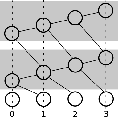
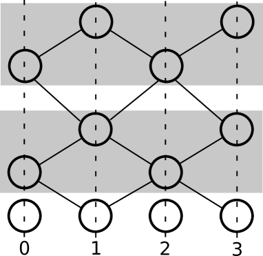
(a)	(b)

Figure 2: 2-layer MFNs for a chain model \raisebox{-.9pt} {0}⃝-\raisebox{-.9pt} {1}⃝-\raisebox{-.9pt} {2}⃝-\raisebox{-.9pt} {3}⃝ with (a) sequential update schedule, (b) block parallel update schedule. The arrows, weights and biases are dropped. The grey plates indicate layers. The height of a node indicates its order in the updates.

From the feed-forward network point of view, MFNs are just a special type of feed-forward networks, with a few important restrictions on the network:

• The weights and biases, or equivalently the parameter $\theta$’s, on all layers are tied and equal to the $\theta$ in the underlying pairwise MRF.

• The network structure is the same on all layers and follows the structure of the pairwise MRF.

These two restrictions make $M$-layer MFNs exactly equivalent to $M$ iterations of the mean field algorithm. But from the feed-forward network viewpoint, nothing stops us from relaxing the restrictions, as long as we keep the number of outputs at the top layer constant.

By relaxing the restrictions, we lose the equivalence to mean field, but if all we care about is the quality of the input-to-output mapping, measured by some loss function like KL-divergence, then this relaxation can be beneficial. We discuss a few relaxations here that aim to improve $M$-layer MFNs with fixed $M$ as an inference tool for a pairwise MRF with fixed $\theta$:

(1) Untying $\theta$’s in MFNs from the $\theta$ in the original pairwise MRF. If we consider $M$-layer MFNs with fixed $M$, then this relaxation can be beneficial as the mean field algorithm is designed to run until convergence, but not for a specific $M$. Therefore chosing some $\theta^{\prime}\neq\theta$ may lead to better KL-divergence in $M$ steps when $M$ is small. This can save time as the same quality outputs are obtained with less steps. As $M$ grows, we expect the optimal $\theta^{\prime}$ to approach $\theta$.

(2) Untying $\theta$’s on all layers, i.e. allow different $\theta$’s on different layers. This will create a strictly more powerful model with many more parameters. The $\theta$’s on different layers can therefore focus on different things; for example, the lower layers can focus on getting to a good area quickly and the higher layers can focus on converging to an optimum fast.

(3) Untying the network structure from the underlying graphical model. If we remove connections from the MFNs, the forward pass in the network can be faster. If we add connections, we create a strictly more powerful model. Information flows faster on networks with long range connections, which is usually helpful. We can further untie the network structure on all layers, i.e. allow different layers to have different connection structures. This creates a strictly more flexible model.

As an example, we consider relaxation (1) for a trained pairwise CRF with parameter $\theta$. As the model is conditioned on input data, the potentials will be different for each data case, but the same parameter $\theta$ is used to compute the potentials. The aim here is to use a different set of parameters $\theta^{\prime}$ in MFNs to speed up inference for the CRF with parameter $\theta$ at test time, or equivalently to obtain better outputs within a fixed inference budget. To get $\theta^{\prime}$, we compute the potentials for all data cases first using $\theta$. Then the distributions defined by these potentials are used as targets, and we train our MFN to minimize the KL-divergence between the outputs and the targets. Using KL-divergence as the loss function, this training can be done by following the gradients of $\theta^{\prime}$, which can be computed by the standard back-propagation algorithm developed for feed-forward networks. To be more specific, the KL-divergence loss is defined as

$$\mathrm{KL}(q^{M}||p)=\sum_{s\in\mathcal{V}}\sum_{x_{s}\in\mathcal{X}}q^{M}_{s}(x_{s})\log q^{M}_{s}(x_{s})-\sum_{s\in\mathcal{V}}\sum_{x_{s}\in\mathcal{X}}q^{M}_{s}(x_{s})f_{s}(x_{s})$$

$$-\sum_{(s,t)\in\mathcal{E}}\sum_{x_{s},x_{t}\in\mathcal{X}}q^{M}_{s}(x_{s})q^{M}_{t}(x_{t})f_{st}(x_{s},x_{t})+C$$ (4)

where $q^{M}$ is the $M$th layer output and $C$ is a constant representing terms that do not depend on $q^{M}$. The gradient of the loss with respect to $q^{M}_{s}(x_{s})$ can be computed as

$$\frac{\partial{\mathrm{KL}}}{\partial{q^{M}_{s}(x_{s})}}=\log q^{M}_{s}(x_{s})+1-f_{s}(x_{s})-\sum_{t\in\mathcal{N}(s)}\sum_{x_{t}\in\mathcal{X}}q^{M}_{t}(x_{t})f_{st}(x_{s},x_{t})$$ (5)

The gradient with respect to $\theta^{\prime}$ follows from the chain rule, as $q^{M}$ is a function of $\theta^{\prime}$.

At test time, $\theta^{\prime}$ instead of $\theta$ is used to compute the outputs, which is expected to get to the same results as using mean field in fewer steps.

The discussions above focus on making MFNs better tools for inference. We can, however, take a step even further, to abandon the underlying pairwise MRF and use MFNs directly as discriminative models. For this setting, MFNs correspond to conditional distributions of form $q_{\theta^{\prime}}(\mathbf{x}|\mathbf{y})$ where $\mathbf{y}$ is some input and $\theta^{\prime}$ is the parameters. The $q$ distribution is factorial, and defined by a forward pass of the network. The weights and biases on all layers as well as the initial distribution at the bottom layer can depend on $\mathbf{y}$ via functions with parameters $\theta^{\prime}$. These discriminative MFNs can be learned using a training set of $(\hat{\mathbf{x}},\hat{\mathbf{y}})$ pairs to minimize some loss function. An example is the element-wise hinge loss, which is better defined on inputs to the output layers $a^{*}_{s}(x_{s})=f_{s}(x_{s})+\sum_{t\in\mathcal{N}(s)}\sum_{x_{t}}q_{t}(x_{t})f_{st}(x_{s},x_{t})$, i.e. the exponent part in Eq. 3

$$L(a^{M},\hat{\mathbf{x}})=\sum_{s\in\mathcal{V}}\left[\max_{k}\left\{a^{M}_{s}(k)+\Delta(k,\hat{y}_{s})\right\}-a^{M}_{s}(\hat{y}_{s})\right]$$ (6)

where $\Delta$ is the task loss function. An example is $\Delta(k,\hat{y}_{s})=c\mathbf{I}[k\neq\hat{y}_{s}]$, where $c$ is the loss for mislabeling and $\mathbf{I}[.]$ is the indicator function. The gradient of this loss with respect to $a^{M}$ has a very simple form

$$\frac{\partial{L}}{\partial{a^{M}_{s}(k)}}=\mathbf{I}[k=k^{*}]-\mathbf{I}[k=\hat{y}_{s}]$$ (7)

where $k^{*}=\operatorname*{argmax}_{k}\left\{a^{M}_{s}(k)+\Delta(k,\hat{y}_{s})\right\}$. The gradient of $\theta^{\prime}$ can then be computed using back-propagation.

Compared to the standard paradigm that uses intractable inference during learning, these discriminative MFNs are trained with fixed inference budget ($M$ steps/layers) in mind, and therefore can be expected to work better when we only run the inference for a fixed number of steps. The discriminative formulation also enables the use of a variety of different loss functions more suitable for discriminative tasks like the hinge loss defined above, which is usually not straight-forward to be integrated into the standard paradigm. Many relaxations described before can be used here to make the discriminative model more powerful, for example untying weights on different layers.

2 Related Works

Previous work by Justin Domke (Domke, 2011, 2013) and Stoyanov et al.(Stoyanov et al., 2011) are the most related to ours. In (Domke, 2011, 2013), the author described the idea of truncating message-passing at learning and test time to a fixed number of steps, and back-propagating through the truncated inference procedure to update parameters of the underlying graphical model. In (Stoyanov et al., 2011) the authors proposed to train graphical models in a discriminative fashion to directly minimize empirical risk, and used back-propagation to optimize the graphical model parameters.

Compared to their approaches, our MFN model is one step further. The MFNs have a more explicit connection to feed-forward neural networks, which makes it clear to see where the restrictions of the model are, and also more straight-forward to derive gradients for back-propagation. MFNs enables some natural relaxations of the restrictions like weight sharing, which leads to faster and better inference as well as more powerful prediction models. When restricting our MFNs to have the same weights and biases on all layers and tied to the underlying graphical model, we can recover the method in (Domke, 2011, 2013) for mean field.

Another work by (Jain, 2007) briefly draws a connection between mean field inference of a specific binary MRF with neural networks, but did not explore further variations.

A few papers have discussed the compatibility between learning and approximate inference algorithms theoretically. (Wainwright, 2006) shows that inconsistent learning may be beneficicial when approximate inference is used at test time, as long as the learning and test time inference are properly aligned. (Kulesza & Pereira, 2007) on the other hand shows that even when using the same approximate inference algorithm at training and test time can have problematic results when the learning algorithm is not compatible with inference. MFNs do not have this problem, as training follows the exact gradient of the loss function.

On the neural networks side, people have tried to use a neural network to approximate intractable posterior distributions for a long time, especially for learning sigmoid belief networks, see for example (Dayan et al., 1995) and recent paper (Mnih & Gregor, 2014) and citations therein. As far as we know, no previous work on the neural network side have discussed the connection with mean field or belief propagation type methods used for variational inference in graphical models.

A recent paper (Korattikara et al., 2014) develops approximate MCMC methods with limited inference budget, which shares the spirit of our work.

3 Preliminary Experiment Results

We demonstrate the performance of MFNs on an image denoising task. We generated a synthetic dataset of 50$\times$100 images. Each image has a black background (intensity 0) and some random white (intensity 1) English letters as foreground. Then flipping noise (pixel intensity fliped from 0 to 1 or 1 to 0) and Gaussian noise are added to each pixel. The task is to recover the clean text images from the noisy images, more specifically, to label each pixel into one of two classes: foreground or background. In this way it is also a binary segmentation problem. We generated training and test sets, each containing 50 images. A few example images and corresponding labels are shown in Fig. 3.

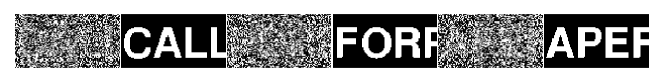
Figure 3: Three pairs of example images, in each pair: left image is the noisy input image, right image is the ground truth label.

The baseline model we consider in the experiments is a pairwise CRF. The model defines a posterior distribution of output label $\mathbf{x}$ given input image $\mathbf{y}$. For each pixel $s$ the label $x_{s}\in\{0,1\}$. The conditional unary potentials are defined using a linear model $f_{s}(x_{s};\mathbf{y})=x_{s}\mathbf{w}^{\top}\phi(\mathbf{y},s)$, where $\phi(\mathbf{y},s)$ extracts a 5$\times$5 window around pixel $s$ and padded with a constant 1 to form a 26-dimensional feature vector, $\mathbf{w}$ is the parameter vector for unary potentials. The pairwise potentials are defined as Potts potentials, $f_{st}(x_{s},x_{t};\mathbf{y})=p_{st}\mathbf{I}[x_{s}=x_{t}]$, where $p_{st}$ is the penalty for pixel $s$ and $t$ to take different labels. We use one single penalty $p_{h}$ for all horizontal edges and another $p_{v}$ for all vertical edges. In total, the baseline model specified by $\theta=(\mathbf{w},p_{h},p_{v})$ has 28 parameters.

For all inference procedures in the experiments for both mean field and MFNs, the distributions are initialized by taking softmax of unary potentials.

We learn $\theta$ for the baseline model by gradient ascent to maximize the conditional log likelihood of training data. To compute the gradients, the posterior expectations are approximated using marginals obtained by running mean field for 30 steps (abbrev. MF-30). $\theta$ is initialized as an all 1 vector, except that the weight for constant feature in unary model is set to $-5\times 5/2=-12.5$. We denote this initial parameter setting as $\theta_{0}$, and the parameters after training as $\theta_{\mathrm{MF}}$. With MF-30, $\theta_{0}$ achieves an accuracy of 0.7957 on test set, after training, the accuracy improves to 0.8109.

3.1 MFN for Inference

In the first experiment, we learn MFNs to do inference for the CRF model with parameter $\theta_{\mathrm{MF}}$. We train $M$-layer MFNs (MFN-$M$) with fully untied weights on all layers to minimize the KL-divergence loss for $M=1,3,10,30$. The MFN parameters on all layers are initialized to be the same as $\theta_{\mathrm{MF}}$.

As baselines, the average KL-divergence on test set using MF-1, MF-3, MF-10 and MF-30 are $-12779.05$, $-12881.50$, $-12904.43$, $-12908.54$. Note these numbers are the KL-divergence without the constant corresponding to log-partition function, which we cannot compute. The corresponding KL-divergence on test set for MFN-1, MFN-3, MFN-10, MFN-30 are $-12837.87$, $-12893.52$, $-12908.80$, $-12909.34$. We can see that MFNs improve performance more significantly when $M$ is small, and MFN-10 is even better than MF-30, while MF-30 runs the inference for 20 more iterations than MFN-10.

3.2 MFN as Discriminative Model

In the second experiment, we train MFNs as discriminative models for the denoising task directly. We start with a three-layer MFN with tied weights (MFN-3-t). The MFN parameters are initialized to be the same as $\theta_{\mathrm{MF}}$. As baselines, MF-3 with $\theta_{\mathrm{MF}}$ achieves an accuracy of 0.8065 on test set, and MF-30 with $\theta_{0}$ and $\theta_{\mathrm{MF}}$ achieves accuracy 0.7957 and 0.8109 respectively as mentioned before.

We learn MFN-3-t to minimize the element-wise hinge loss with learning rate 0.0005 and momentum 0.5. After 50 gradient steps, the test accuracy improves and converges to around 0.8134, which beats all the mean field baselines and is even better than MF-30 with $\theta_{\mathrm{MF}}$.

Then we untie the weights of the three-layer MFN (denoted MFN-3) and continue training with larger learning rate 0.002 and momentum 0.9 for another 200 steps. The test accuracy improves further to around 0.8151. During learning, we observe that the gradients for the three layers are usually quite different: the first and third layer gradients are usually much larger than the second layer gradients. This may cause a problem for MFN-3-t, which is essentially using the same gradient (sum of gradients on three layers) for all three layers.

As a comparison, we tried to continue training MFN-3-t without untying the weights using learning rate 0.002 and momentum 0.9. The test accuracy improves to around 0.8145 but oscillated a lot and eventually diverged. We’ve tried a few smaller learning rate and momentum settings but can not get the same level of performance as MFN-3 within 200 steps.

4 Discussion and Ongoing Work

In this paper we proposed the Mean Field Networks, based on a feed-forward network view of the mean field algorithm with fixed number of iterations. We show that relaxing the restrictions on MFNs can improve inference efficiency and discriminative performance. There are a lot of possible extensions around this model and we are working on a few of them: (1) integrate learning graphical model and learning inference model together; (2) relaxing the network structure restrictions; (3) extend the method to other inference algorithms like belief propagation.

References

- Dayan et al. (1995) Dayan, P., Hinton, G.E., Neal, R.M., and Zemel, R.S. The helmholtz machine. Neural computation, 7(5):889–904, 1995.
- Domke (2011) Domke, Justin. Parameter learning with truncated message-passing. In IEEE Conference on Computer Vision and Pattern Recognition (CVPR), pp. 2937–2943, 2011.
- Domke (2013) Domke, Justin. Learning graphical model parameters with approximate marginal inference. IEEE Transactions on Pattern Analysis and Machine Intelligence, 2013.
- Jain (2007) Jain, Viren et al. Supervised learning of image restoration with convolutional networks. In International Conference on Computer Vision (ICCV), 2007.
- Korattikara et al. (2014) Korattikara, Anoop, Chen, Yutian, and Welling, Max. Austerity in mcmc land: Cutting the metropolis-hastings budget. In International Conference on Machine Learning (ICML), 2014.
- Kulesza & Pereira (2007) Kulesza, Alex and Pereira, Fernando. Structured learning with approximate inference. In NIPS, volume 20, pp. 785–792, 2007.
- Mnih & Gregor (2014) Mnih, Andriy and Gregor, Karol. Neural variational inference and learning in belief networks. arXiv preprint arXiv:1402.0030, 2014.
- Stoyanov et al. (2011) Stoyanov, Veselin, Ropson, Alexander, and Eisner, Jason. Empirical risk minimization of graphical model parameters given approximate inference, decoding, and model structure. In International Conference on Artificial Intelligence and Statistics (AISTATS), pp. 725–733, 2011.
- Wainwright (2006) Wainwright, Martin J. Estimating the wrong graphical model: Benefits in the computation-limited setting. Journal of Machine Learning Research (JMLR), 7:1829–1859, 2006.