A geometric approach to the optimal control of nonholonomic mechanical systems

Abstract.

In this paper, we describe a constrained Lagrangian and Hamiltonian formalism for the optimal control of nonholonomic mechanical systems. In particular, we aim to minimize a cost functional, given initial and final conditions where the controlled dynamics is given by nonholonomic mechanical system. In our paper, the controlled equations are derived using a basis of vector fields adapted to the nonholonomic distribution and the Riemannian metric determined by the kinetic energy. Given a cost function, the optimal control problem is understood as a constrained problem or equivalently, under some mild regularity conditions, as a Hamiltonian problem on the cotangent bundle of the nonholonomic distribution. A suitable Lagrangian submanifold is also shown to lead to the correct dynamics. We demonstrate our techniques in several examples including a continuously variable transmission problem and motion planning for obstacle avoidance problems.

Dedicated to Hélene Frankowska and Héctor J. Sussmann

1. Introduction

Although nonholonomic systems have been studied since the dawn of analytical mechanics, there has been some confusion over the correct formulation of the equations of motion (see e.g. [4], [10] and [29] for some of the history). Further it is only recently that their geometric formulation has been understood. In addition, there has been recent interest in the analysis of control problems for such systems. Nonholonomic control systems exhibit distinctive features. In particular, many naturally underactuated systems are controllable, the controllability arising from the nonintegrability of the constraints.

Nonholonomic optimal control problems arise in many engineering applications, for instance systems with wheels, such as cars and bicycles, and systems with blades or skates. There are thus multiple applications in the context of wheeled motion, space or mobile robotics and robotic manipulation. In this paper, we will introduce some new geometric techniques in nonholonomic mechanics to study the case of force minimizing optimal control problems.

The application of modern tools from differential geometry in the fields of mechanics, control theory, field theory and numerical integration has led to significant progress in these research areas. For instance, the study of the geometrical formulation of the nonholonomic equations of motion has led to better understanding of different engineering problems such locomotion generation, controllability, motion planning, and trajectory tracking (see e.g. [4], [5], [6], [7], [8], [12], [13], [24], [25], [30], [31], [32], [39], [41] and references therein). Geometric techniques can also be used to study optimal control problems (see [8], [15], [16], [22], [23], [45], [46]). Combining these ideas in this paper, we study the underlying geometry of optimal control problems for mechanical systems subject to nonholonomic constraints and we apply it to several interesting examples.

Classical nonholonomic constraints which are linear in the velocities can be geometrically encoded by a constant rank distribution $\mathcal{D}$. As we will see, the distribution $\mathcal{D}$ will play the role of the velocity phase space. Given a mechanical Lagrangian $L=K-V:TQ\rightarrow{\mathbb{R}}$ where $K$ and $V$ are the kinetic and potential energy, respectively. and the distribution ${\mathcal{D}}$, the dynamics of the nonholonomic system is completely determined using the Lagrange-d’Alembert principle [4]. In this paper we will formulate a description in terms of a Levi Civita connection defined on the space of vector fields taking values on ${\mathcal{D}}$. This connection is obtained by projecting the standard Lie bracket using the Riemannian metric associated with the kinetic energy $K$ (see [3]) and the typical characterization of the Levi-Civita connection (see also [9]). By adding controls in this setting we can study optimal control problems such as the force minimizing problem. Moreover, we can see that the dynamics of the optimal control problem is completely described by a Lagrangian submanifold of an appropriate cotangent bundle and, under some regularity conditions, the equations of motion are derived as classical Hamilton’s equations on the cotangent bundle of the distribution, $T^{*}{\mathcal{D}}$. Although our approach is intrinsic, we also give a local description since it is important for working out examples. For this, it is necessary to choose an adapted basis of vector fields for the distribution. From this point of view, we combine the techniques used previously by the authors of the paper (see [3], [11], [37]). An additional advantage of our method is that symmetries may be naturally analyzed in this setting.

Concretely, the main results of our paper can be summarized as follows:

• Geometric derivation of the equations of motion of nonholonomic optimal control problems as a constrained problem on the tangent space to the constraint distribution ${\mathcal{D}}$.

• Construction of a Lagrangian submanifold representing the dynamics of the optimal control problem and the corresponding Hamiltonian representation when the system is regular.

• Definition of a Legendre transformation establishing the relationship and correspondence between the Lagrangian and Hamiltonian dynamics.

• Application of our techniques to different examples including optimal control of the Chaplygin sleigh, a continuously variable transmission and motion planning for obstacle avoidance problems.

2. Nonholonomic mechanical systems

Constraints on mechanical systems are typically divided into two types: holonomic and nonholonomic, depending on whether the constraint can be derived from a constraint in the configuration space or not. Therefore, the dimension of the space of configurations is reduced by holonomic constraints but not by nonholonomic constraints. Thus, holonomic constraints allow a reduction in the number of coordinates of the configuration space needed to formulate a given problem (see [40]).

We will restrict ourselves to the case of nonholonomic constraints. Additionally, assume that the constraints are given by a nonintegrable distribution $\mathcal{D}$ on the configuration space $Q$. Locally, if we choose local coordinates $(q^{i})$, $1\leq i\leq n=\dim Q$, the linear constraints on the velocities are locally given by equations of the form

$$\phi^{a}(q^{i},\dot{q}^{i})=\mu^{a}_{i}(q)\dot{q}^{i}=0,\quad 1\leq a\leq m\leq n,$$

depending, in general, on configuration coordinates and their velocities. From an intrinsic point of view, the linear constraints are defined by a distribution ${\mathcal{D}}$ on $Q$ of constant rank $n-m$ such that the annihilator of ${\mathcal{D}}$ is locally given by

$${\mathcal{D}}^{o}=\operatorname{span}\left\{\mu^{a}=\mu_{i}^{a}dq^{i}\;;1\leq a\leq m\right\}$$

where the 1-forms $\mu^{a}$ are independent.

In addition to these constraints, we need to specify the dynamical evolution of the system, usually by fixing a Lagrangian function $L\colon TQ\to\mathds{R}$. In mechanics, the central concepts permitting the extension of mechanics from the Newtonian point of view to the Lagrangian one are the notions of virtual displacements and virtual work; these concepts were originally formulated in the developments of mechanics in their application to statics. In nonholonomic dynamics, the procedure is given by the Lagrange–d’Alembert principle. This principle allows us to determine the set of possible values of the constraint forces from the set $\mathcal{D}$ of admissible kinematic states alone. The resulting equations of motion are

$$\left[\frac{d}{dt}\left(\frac{\partial L}{\partial\dot{q}^{i}}\right)-\frac{\partial L}{\partial q^{i}}\right]\delta q^{i}=0,$$

where $\delta q^{i}$ denotes the virtual displacements verifying

$$\mu^{a}_{i}\delta q^{i}=0$$

(for the sake of simplicity, we will assume that the system is not subject to non-conservative forces). This must be supplemented by the constraint equations. By using the Lagrange multiplier rule, we obtain

$$\frac{d}{dt}\left(\frac{\partial L}{\partial\dot{q}^{i}}\right)-\frac{\partial L}{\partial q^{i}}={\lambda}_{a}\mu^{a}_{i}.$$

The term on the right hand side represents the constraint force or reaction force induced by the constraints. The functions $\lambda_{a}$ are Lagrange multipliers which, after being computed using the constraint equations, allow us to obtain a set of second order differential equations.

Now we restrict ourselves to the case of nonholonomic mechanical systems where the Lagrangian is of mechanical type

$$L(v_{q})=\frac{1}{2}\mathcal{G}(v_{q},v_{q})-V(q),\quad v_{q}\in T_{q}Q.$$

Here $\mathcal{G}$ denotes a Riemannian metric on the configuration space $Q$ representing the kinetic energy of the systems and $V:Q\rightarrow\mathds{R}$ is a potential function. Locally, the metric is determined by the matrix $M=(\mathcal{G}_{ij})_{1\leq i,j\leq n}$ where $\mathcal{G}_{ij}=\mathcal{G}(\partial/\partial q^{i},\partial/\partial q^{j})$.

Denote by $\tau_{\mathcal{D}}:\mathcal{D}\rightarrow Q$ the canonical projection of $\mathcal{D}$ over $Q$ and $\Gamma(\tau_{\mathcal{D}})$ the set of sections of $\tau_{D}$ which is just the set of vector fields $\mathfrak{X}(Q)$ taking values on $\mathcal{D}.$ If $X,Y\in\mathfrak{X}(Q),$ then $[X,Y]$ denotes the standard Lie bracket of vector fields.

Definition 2.1.

A nonholonomic mechanical system on a manifold $Q$ is given by the triple $(\mathcal{G},V,\mathcal{D})$ where $\mathcal{G}$ is a Riemannian metric on $Q,$ specifying the kinetic energy of the system, $V:Q\rightarrow\mathds{R}$ is a smooth function representing the potential energy and $\mathcal{D}$ a non-integrable distribution on $Q$ representing the nonholonomic constraints.

Remark 2.2.

Given $X,Y\in\Gamma(\tau_{\mathcal{D}})$ that is, $X(x)\in\mathcal{D}_{x}$ and $Y(x)\in\mathcal{D}_{x}$ for all $x\in Q,$ then it may happen that $[X,Y]\notin\Gamma(\tau_{\mathcal{D}})$ since $\mathcal{D}$ is nonintegrable.

We want to obtain a bracket defined for sections of $\mathcal{D}.$ Using the Riemannian metric $\mathcal{G}$ we can construct two complementary orthogonal projectors

$${\mathcal{P}}\colon TQ\to{\mathcal{D}}$$

$${\mathcal{Q}}\colon TQ\to{\mathcal{D}}^{\perp},$$

with respect to the tangent bundle orthogonal decomposition $\mathcal{D}\oplus\mathcal{D}^{\perp}=TQ.$

Therefore, given $X,Y\in\Gamma(\tau_{\mathcal{D}})$ we define the nonholonomic bracket $[\![\cdot,\cdot]\!]:\Gamma(\tau_{\mathcal{D}})\times\Gamma(\tau_{\mathcal{D}})\rightarrow\Gamma(\tau_{\mathcal{D}})$ as

$$[\![X,Y]\!]:=\mathcal{P}[X,Y]\;,\qquad X,Y\in\Gamma(\tau_{\mathcal{D}})$$

(see [2],[3],[19]). It is clear that this Lie bracket verifies the usual properties of a Lie bracket except the Jacobi identity.

Remark 2.3.

From a more differential geometric point of view, ${\mathcal{D}}$ with this modified bracket of sections inherits a skew-symmetric Lie algebroid structure [20, 3] where now the bracket of sections of the vector bundle does not satisfy in general the Jacobi identity, as an expression of the nonintegrability of the distribution ${\mathcal{D}}$.

Definition 2.4.

Consider the restriction of the Riemannian metric $\mathcal{G}$ to the distribution $\mathcal{D}$

$$\mathcal{G}^{\mathcal{D}}:\mathcal{D}\times_{Q}\mathcal{D}\rightarrow\mathds{R}$$

and define the Levi-Civita connection

$$\nabla^{\mathcal{G}^{\mathcal{D}}}:\Gamma(\tau_{\mathcal{D}})\times\Gamma(\tau_{\mathcal{D}})\rightarrow\Gamma(\tau_{\mathcal{D}})$$

determined by the following two properties:

1. $[\![X,Y]\!]=\nabla_{X}^{\mathcal{G}^{\mathcal{D}}}Y-\nabla_{Y}^{\mathcal{G}^{\mathcal{D}}}X$ (Symmetry),
   

2. $X(\mathcal{G}^{\mathcal{D}}(Y,Z))=\mathcal{G}^{\mathcal{D}}(\nabla_{X}^{\mathcal{G}^{\mathcal{D}}}Y,Z)+\mathcal{G}^{\mathcal{D}}(Y,\nabla_{X}^{\mathcal{G}^{\mathcal{D}}}Z)$ (Metricity).

Let $(q^{i})$ be coordinates on $Q$ and $\{e_{A}\}$ vector fields on $\Gamma(\tau_{D})$ (that is, $e_{A}(x)\in{\mathcal{D}}_{x}$) such that

$$\mathcal{D}_{x}=\hbox{span }\{e_{A}(x)\},\quad x\in U\subset Q.$$

Then, we determine the Christoffel symbols $\Gamma_{BC}^{A}$ of the connection $\nabla^{\mathcal{G}^{\mathcal{D}}}$ by

$$\nabla_{e_{B}}^{\mathcal{G}^{\mathcal{D}}}e_{C}=\Gamma_{BC}^{A}(q)e_{A}.$$

Definition 2.5.

A curve $\gamma:I\subset\mathds{R}\rightarrow\mathcal{D}$ is admissible if there exists a curve $\sigma:I\subset\mathds{R}\rightarrow Q$ projecting $\gamma$ over $Q,$ that is, $\tau_{\mathcal{D}}\circ\gamma=\sigma;$ such that

$$\gamma(t)=\frac{d\sigma}{dt}(t).$$

Given local coordinates on $Q,$ $(q^{i})$ $i=1,\ldots,n;$ and $\{e_{A}\}$ a basis of sections on $\Gamma(\tau_{\mathcal{D}})$ such that $\displaystyle{e_{A}=\rho_{A}^{i}(q)\frac{\partial}{\partial q^{i}}}$ we introduce induced coordinates $(q^{i},y^{A})$ on $\mathcal{D}$ where, if $e\in\mathcal{D}_{x}$ then $e=y^{A}e_{A}(x).$ Therefore, $\gamma(t)=(q^{i}(t),y^{A}(t))$ is admissible if

$$\dot{q}^{i}(t)=\rho_{A}^{i}(q(t))y^{A}(t).$$

Consider the restricted Lagrangian function $\ell:\mathcal{D}\rightarrow\mathbb{R},$

$$\ell(v)=\frac{1}{2}\mathcal{G}^{\mathcal{D}}(v,v)-V(\tau_{D}(v)),\hbox{ with }v\in\mathcal{D}.$$

Definition 2.6 ([3]).

A solution of the nonholonomic problem is an admissible curve $\gamma:I\rightarrow\mathcal{D}$ such that

$$\nabla_{\gamma(t)}^{\mathcal{G}^{\mathcal{D}}}\gamma(t)+grad_{\mathcal{G}^{\mathcal{D}}}V(\tau_{\mathcal{D}}(\gamma(t)))=0.$$

Here the section $grad_{{\mathcal{G}}^{\mathcal{D}}}V\in\Gamma(\tau_{\mathcal{D}})$ is characterized by

$${{\mathcal{G}}^{\mathcal{D}}}(grad_{{\mathcal{G}}^{\mathcal{D}}}V,X)=X(V),\;\;\mbox{ for every }X\in\Gamma(\tau_{\mathcal{D}}).$$

These equations are equivalent to the nonholonomic equations. Locally, these are given by

$$\dot{q}^{i} = \rho_{A}^{i}(q)y^{A}$$

$$\dot{y}^{C} = -\Gamma_{AB}^{C}y^{A}y^{B}-(\mathcal{G}^{\mathcal{D}})^{CB}\rho_{B}^{i}\frac{\partial V}{\partial q^{i}}$$

where $(\mathcal{G}^{\mathcal{D}})^{AB}$ denotes the coefficients of the inverse matrix of $(\mathcal{G}^{\mathcal{D}})_{AB}$ where $\mathcal{G}^{\mathcal{D}}(e_{A},e_{B})=(\mathcal{G}^{\mathcal{D}})_{AB}.$

Remark 2.7.

Observe that these equations only depend on the coordinates $(q^{i},y^{A})$ on $\mathcal{D}$. Therefore the nonholonomic equations are free of Lagrange multipliers. These equations are equivalent to the nonholonomic Hamel equations (see [11], [37] for example, and reference therein).

3. Optimal control of nonholonomic mechanical systems

The purpose of this section is to study optimal control problems for a nonholonomic mechanical systems. We shall assume that all the considered control systems are controllable, that is, for any two points $q_{0}$ and $q_{f}$ in the configuration space $Q$, there exists an admissible control $u(t)$ defined on the control manifold $U\subseteq\mathds{R}^{n}$ such that the system with initial condition $q_{0}$ reaches the point $q_{f}$ at time $T$ (see [4, 13] for more details).

We will analyze the case when the dimension of the input or control distribution is equal to the rank of ${\mathcal{D}}$. If the rank of $\mathcal{D}$ is equal to the dimension of the control distribution, the system will be called a fully actuated nonholonomic system.

Definition 3.1.

A solution of a fully actuated nonholonomic problem is an admissible curve $\gamma:I\rightarrow\mathcal{D}$ such that

$$\nabla_{\gamma(t)}^{\mathcal{G}^{\mathcal{D}}}\gamma(t)+grad_{\mathcal{G}^{\mathcal{D}}}V(\tau_{\mathcal{D}}(\gamma(t)))\in\Gamma(\tau_{D}),$$

or, equivalently,

$$\nabla_{\gamma(t)}^{\mathcal{G}^{\mathcal{D}}}\gamma(t)+grad_{\mathcal{G}^{\mathcal{D}}}V(\tau_{\mathcal{D}}(\gamma(t)))=u^{A}(t)e_{A}(\tau_{\mathcal{D}}(\gamma(t)),$$

where $u^{A}$ are the control inputs.

Locally, the equations may be written as

$$\dot{q}^{i} = \rho_{A}^{i}y^{A}$$

$$\dot{y}^{C} = -\Gamma_{AB}^{C}y^{A}y^{B}-(\mathcal{G}^{\mathcal{D}})^{CB}\rho_{B}^{i}\frac{\partial V}{\partial q^{i}}+u^{C}.$$

Given a cost function

$$C : \mathcal{D}\times U\rightarrow\mathbb{R}$$

$$(q^{i},y^{A},u^{A})\mapsto C(q^{i},y^{A},u^{A})$$

the optimal control problem consists of finding an admissible curve $\gamma:I\rightarrow\mathcal{D}$ solution of the fully actuated nonholonomic problem given initial and final boundary conditions on $\mathcal{D}$ and minimizing the functional

$$\mathcal{J}(\gamma(t),u(t)):=\int_{0}^{T}C(\gamma(t),u(t))dt,$$

where $\gamma$ is an admissible curve.

We define the submanifold $\mathcal{D}^{(2)}$ of $T\mathcal{D}$ by

$$\mathcal{D}^{(2)}:=\{v\in T\mathcal{D}\mid v=\dot{\gamma}(0)\hbox{ where }\gamma:I\rightarrow\mathcal{D}\hbox{ is admissible}\},$$ (1)

and we can choose coordinates $(x^{i},y^{A},\dot{y}^{A})$ on $\mathcal{D}^{(2)}$ where the inclusion on $T\mathcal{D}$, $i_{\mathcal{D}^{(2)}}:\mathcal{D}^{(2)}\hookrightarrow T\mathcal{D}$ is given by

$$i_{\mathcal{D}^{(2)}}(q^{i},y^{A},\dot{y}^{A})=(q^{i},y^{A},\rho_{A}^{i}(q)y^{A},\dot{y}^{A}).$$

Therefore, $\mathcal{D}^{(2)}$ is locally described by the constraints on $T\mathcal{D}$

$$\dot{q}^{i}-\rho_{A}^{i}y^{A}=0.$$

Observe now that our optimal control problem is alternatively determined by a smooth function $\mathcal{L}:\mathcal{D}^{(2)}\rightarrow\mathbb{R}$ where

$$\mathcal{L}(q^{i},y^{A},\dot{y}^{C})=C\left(q^{i},y^{A},\dot{y}^{C}+\Gamma_{AB}^{C}y^{A}y^{B}+(\mathcal{G}^{\mathcal{D}})^{CB}\rho_{B}^{i}\frac{\partial V}{\partial q^{i}}\right).$$ (2)

The following diagram summarizes the situation:

Here $j:\mathcal{D}\rightarrow TQ$ is the canonical inclusion from $\mathcal{D}$ to $TQ,$ $\tau_{\mathcal{D}}^{(2,1)}:\mathcal{D}^{(2)}\rightarrow\mathcal{D}$ and $\tau_{T\mathcal{D}}:T\mathcal{D}\rightarrow\mathcal{D}$ are the projections locally given by $\tau_{\mathcal{D}}^{(2,1)}(q^{i},y^{A},\dot{y}^{A})=(q^{i},y^{A})$ and $\tau_{T\mathcal{D}}(q^{i},y^{A},v^{i},\dot{y}^{A})=(q^{i},y^{A}),$ respectively. Finally, $T\tau_{\mathcal{D}}:T\mathcal{D}\rightarrow TQ$ is locally described as follows $(q^{i},y^{A},\dot{q}^{i},\dot{y}^{A})\mapsto(q^{i},\dot{q}^{i})$.

To derive the equations of motion for $\mathcal{L}$ we can use standard variational calculus for systems with constraints defining the extended Lagrangian $\widetilde{\mathcal{L}},$

$$\widetilde{\mathcal{L}}=\mathcal{L}+\lambda_{i}(\dot{q}^{i}-\rho_{A}^{i}y^{A}).$$

Therefore the equations of motion are

$$\frac{d}{dt}\left(\frac{\partial\widetilde{\mathcal{L}}}{\partial\dot{q}^{i}}\right)-\frac{\partial\widetilde{\mathcal{L}}}{\partial q^{i}} = \dot{\lambda}_{i}-\frac{\partial\mathcal{L}}{\partial q^{i}}+\lambda_{j}\frac{\partial\rho_{A}^{j}}{\partial q^{i}}y^{A}=0,$$

$$\frac{d}{dt}\left(\frac{\partial\widetilde{\mathcal{L}}}{\partial\dot{y}^{A}}\right)-\frac{\partial\widetilde{\mathcal{L}}}{\partial y^{A}} = \frac{d}{dt}\left(\frac{\partial\mathcal{L}}{\partial\dot{y}^{A}}\right)-\frac{\partial\mathcal{L}}{\partial y^{A}}+\rho_{A}^{i}\lambda_{i}=0,$$ (3)

$$\dot{q}^{i} = \rho_{A}^{i}y^{A}.$$

3.1. Example: continuously variable transmission (CVT)

We want to study the optimal control of a simple model of a continuously variable transmissions, where we assume that the belt cannot slip (see [38] for more details).

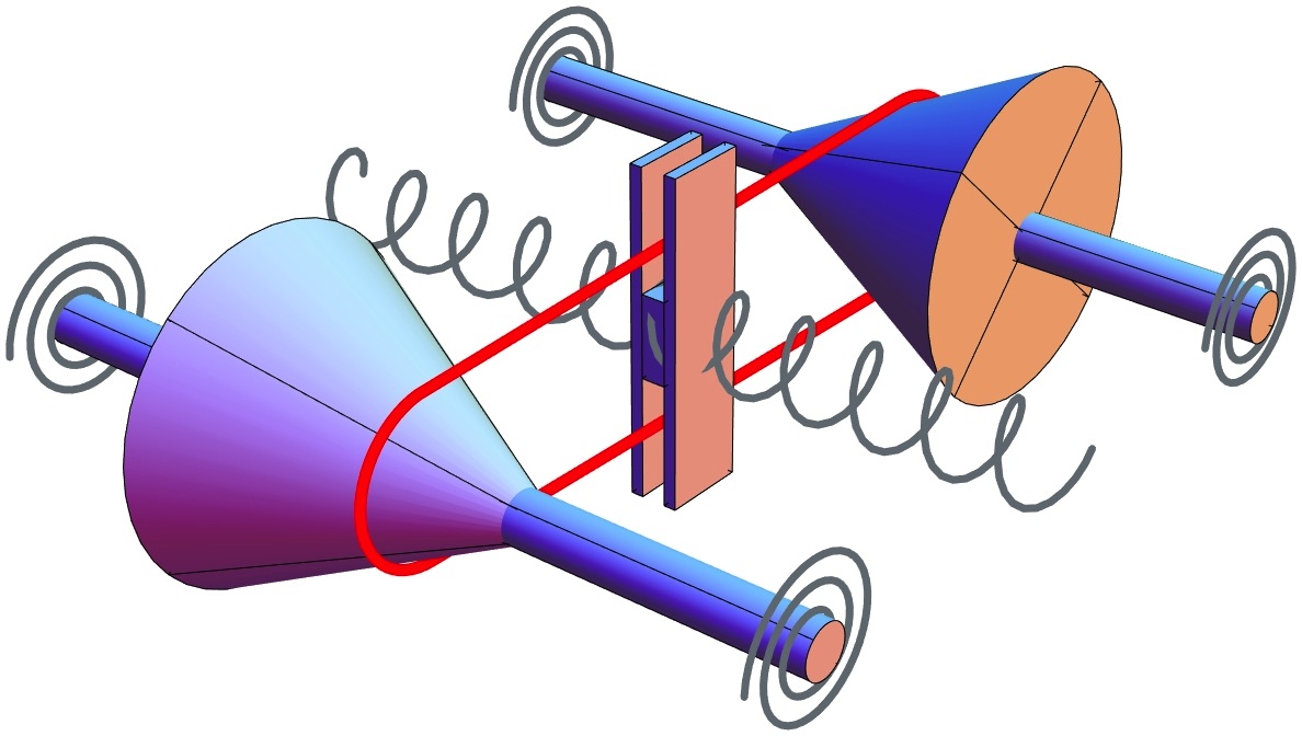
Figure 1. Illustration of a continuously variable transmission [38].

The shafts are attached to spiral springs that are fixed to a chasis. The belt between the two cones is translated along the shafts in accordance with the coordinate $x$, thus providing a varying transmission ratio. The belt is kept in a plane perpendicular to the shafts, so that the belt keeps a constant length (see [38] for a complete description and integrability of this system). The variables $\theta_{1}$ and $\theta_{2}$ denote the angular deflections of the shafts. $m$ denotes the mass of the belt slider, $J_{1}>0$ is the inertia about the center of mass of the driving pulley and $J_{2}>0$ is the inertia about the center of mass of the driven pulley. The configuration space is $\mathbb{S}^{1}\times\mathbb{S}^{1}\times\mathds{R}$ and the configuration is given by $q=(\theta_{1},\theta_{2},x)\in\mathbb{S}^{1}\times\mathbb{S}^{1}\times\mathds{R}$.

The control inputs are denoted by $u_{1}$ and $u_{2}.$ The first one corresponds to a force applied perpendicular to the center of mass of the belt slider and the second one is the torque applied about the the center of mass of the driving pulley. Also, we assume that $x<1$ (which correspond to assuming that the gear ratio is finite).

The belt imposes a constraint given by the no slip condition and is expressed in differential form by

$$\omega=x\,d\theta_{1}-(1-x)\,d\theta_{2}.$$

Therefore the constraint distribution $\mathcal{D}$ is given by

$$\mathcal{D}=\left\{\frac{1}{m}\frac{\partial}{\partial x},(1-x)\frac{\partial}{\partial\theta_{1}}+x\frac{\partial}{\partial\theta_{2}}\right\}.$$

The Lagrangian is metric on $\mathbb{S}^{1}\times\mathbb{S}^{1}\times\mathds{R}$ where the matrix associated with the metric $\mathcal{G}$ is

$$\mathcal{G}=\left(\begin{array}[]{ccc}J_{1}&0&0\\ 0&J_{2}&0\\ 0&0&m\\ \end{array}\right).$$

Then the Lagrangian $L:T(\mathbb{S}^{1}\times\mathbb{S}^{1}\times\mathds{R})\rightarrow\mathds{R}$ is given by

$$L(q,\dot{q})=(\frac{J_{1}}{2}\dot{\theta}_{1}^{2}+\frac{J_{2}}{2}\dot{\theta}_{2}^{2})+\frac{m}{2}\dot{x}^{2}.$$

The projection map $\mathcal{P}:T(\mathbb{S}^{1}\times\mathbb{S}^{1}\times\mathds{R})\rightarrow\mathcal{D}$ is

$$\mathcal{P}(q,\dot{q})=\frac{J_{1}(1-x)^{2}}{J_{1}-2J_{1}x+J_{1}x^{2}+J_{2}x^{2}}d\theta_{1}\otimes\frac{\partial}{\partial\theta_{1}}+\frac{J_{1}x(1-x)}{J_{1}-2J_{1}x+J_{1}x^{2}+J_{2}x^{2}}d\theta_{1}\otimes\frac{\partial}{\partial\theta_{2}}$$

$$+\frac{J_{2}x(1-x)}{J_{1}-2J_{1}x+J_{1}x^{2}+J_{2}x^{2}}d\theta_{2}\otimes\frac{\partial}{\partial\theta_{1}}+\frac{J_{2}x^{2}}{J_{1}-2J_{1}x+J_{1}x^{2}+J_{2}x^{2}}d\theta_{2}\otimes\frac{\partial}{\partial\theta_{2}}+dx\otimes\frac{\partial}{\partial x}.$$

Let $q=(\theta_{1},\theta_{2},x)$ be coordinates on the base manifold $\mathbb{S}^{1}\times\mathbb{S}^{1}\times\mathds{R}$ and take the basis $\{X_{1},X_{2}\}$ of vector fields on $\mathbb{S}^{1}\times\mathbb{S}^{1}\times\mathds{R}.$ This basis induces adapted coordinates $(\theta_{1},\theta_{2},x,y_{1},y_{2})\in\mathcal{D}$ in the following way: Given the vector fields $X_{1}$ and $X_{2}$ generating the distribution $\mathcal{D}$ we obtain the relations for $q\in\mathbb{S}^{1}\times\mathbb{S}^{1}\times\mathbb{R}$

$$X_{1}(q) = \rho_{1}^{1}(q)\frac{\partial}{\partial\theta_{1}}+\rho_{1}^{2}(q)\frac{\partial}{\partial\theta_{2}}+\rho_{1}^{3}(q)\frac{\partial}{\partial x},$$

$$X_{2}(q) = \rho_{2}^{1}(q)\frac{\partial}{\partial\theta_{1}}+\rho_{2}^{2}(q)\frac{\partial}{\partial\theta_{2}}+\rho_{2}^{3}(q)\frac{\partial}{\partial x}.$$

Then,

$$\rho_{1}^{1}=\rho_{1}^{2}=\rho_{2}^{3}=0,\quad\rho_{1}^{3}=\frac{1}{m},\quad\rho_{2}^{1}=1-x,\quad\rho_{2}^{2}=x.$$

Each element $e\in{\mathcal{D}}_{q}$ is expressed as a linear combination of these vector fields:

$$e=y_{1}X_{1}(q)+y_{2}X_{2}(q),\quad q\in\mathbb{S}^{1}\times\mathbb{S}^{1}\times\mathbb{R}.$$

Therefore, the vector subbundle $\tau_{\mathcal{D}}:{\mathcal{D}}\rightarrow\mathbb{S}^{1}\times\mathbb{S}^{1}\times\mathbb{R}$ is locally described by the coordinates $(\theta_{1},\theta_{2},x;y_{1},y_{2})$; the first three for the base and the last two, for the fibers. Observe that

$$e=y_{1}\left(\frac{1}{m}\frac{\partial}{\partial x}\right)+y_{2}\left((1-x)\frac{\partial}{\partial\theta_{1}}+x\frac{\partial}{\partial\theta_{2}}\right)$$

and, in consequence, ${\mathcal{D}}$ is described by the conditions (admissibility conditions):

$$\dot{\theta}_{1}=(1-x)y_{2},\quad\dot{\theta}_{2}=xy_{2},\quad\dot{x}=\frac{1}{m}y_{1}$$

as a vector subbundle of $TQ$ where $y_{1}$ and $y_{2}$ are the adapted velocities relative to the basis of $\mathcal{D}$ defined before.

The nonholonomic bracket is given by $[\![\;,\;]\!]=\mathcal{P}([\cdot,\cdot]).$ Observe now,

$$[\![X_{1},X_{2}]\!]=\mathcal{P}[X_{1},X_{2}] = \mathcal{P}\left(-\frac{1}{m}\frac{\partial}{\partial\theta_{1}}+\frac{1}{m}\frac{\partial}{\partial\theta_{2}}\right)$$

$$= -\frac{1}{m}\frac{J_{1}(1-x)-J_{2}x}{J_{2}x^{2}+J_{1}(1-x)^{2}}\left((1-x)\frac{\partial}{\partial\theta_{1}}+x\frac{\partial}{\partial\theta_{2}}\right).$$

The restricted Lagrangian function in these new adapted coordinates is rewritten as

$$\ell(\theta_{1},\theta_{2},x,y_{1},y_{2})=\frac{y_{2}^{2}}{2}((1-x)^{2}J_{1}+J_{2}x^{2})+\frac{1}{2m}y_{1}^{2}.$$

The Euler-Lagrange equations, together with the admissibility conditions, for this Lagrangian are

$$\frac{\dot{y}_{1}}{m} = 0,\quad\dot{y}_{2}B(x)-\frac{y_{1}y_{2}A(x)}{m}=0$$

$$\dot{\theta}_{1} = (1-x)y_{2},\quad\dot{\theta}_{2}=xy_{2},\quad\dot{x}=\frac{1}{m}y_{1},$$

where $A(x)=J_{1}(1-x)-J_{2}x$ and $B(x)=(1-x)^{2}J_{1}+J_{2}x^{2}$.

Now, we add controls in our picture. Therefore the controlled Euler-Lagrange equations are now

$$u_{1} = \dot{y}_{2}B(x)-\frac{y_{1}y_{2}A(x)}{m},$$

$$u_{2} = \frac{\dot{y}_{1}}{m},$$

together with

$$\dot{\theta}_{1}=(1-x)y_{2},\quad\dot{\theta}_{2}=xy_{2},\quad\dot{x}=\frac{1}{m}y_{1}.$$

The optimal control problem consists of finding an admissible curve satisfying the previous equations given boundary conditions on $\mathcal{D}$ and minimizing the functional

$$\mathcal{J}(\theta_{1},\theta_{2},x,y_{1},y_{2},u_{1},u_{2})=\frac{1}{2}\int_{0}^{T}\left(u_{1}^{2}+u_{2}^{2}\right)dt,$$

for the cost function $C:\mathcal{D}\times U\rightarrow\mathds{R}$ given by

$$C(\theta_{1},\theta_{2},x,y_{1},y_{2},u_{1},u_{2})=\frac{1}{2}(u_{1}^{2}+u_{2}^{2}).$$

This optimal control problem is equivalent to the constrained optimization problem determined by the lagrangian $\mathcal{L}:\mathcal{D}^{(2)}\rightarrow\mathds{R}$ given by

$$\mathcal{L}(\theta_{1},\theta_{2},x,y_{1},y_{2},\dot{y}_{1},\dot{y}_{2}) = \frac{1}{2}\left(\dot{y}_{2}B(x)-\frac{y_{1}y_{2}A(x)}{m}\right)^{2}+\frac{\dot{y}_{1}^{2}}{2m^{2}}.$$

Here, $\mathcal{D}^{(2)}$ is a submanifold of the vector bundle $T\mathcal{D}$ over $\mathcal{D}$ defined by

$$\mathcal{D}^{(2)}:=\left\{(\theta_{1},\theta_{2},x,y_{1},y_{2},\dot{\theta}_{1},\dot{\theta}_{2},\dot{x},\dot{y}_{1},\dot{y}_{2})\in T\mathcal{D}\Big{|}\dot{x}-\frac{1}{m}y_{1}=0,\dot{\theta}_{1}-(1-x)y_{2}=0,\dot{\theta}_{2}-xy_{2}=0\right\},$$

where the inclusion $i_{\mathcal{D}^{(2)}}:\mathcal{D}^{(2)}\hookrightarrow T\mathcal{D},$ is given by the map

$$i_{\mathcal{D}^{(2)}}(\theta_{1},\theta_{2},x,y_{1},y_{2},\dot{y}_{1},\dot{y}_{2})=\left(\theta_{1},\theta_{2},x,y_{1},y_{2},(1-x)y_{2},xy_{2},\frac{y_{1}}{m},\dot{y}_{1},\dot{y}_{2}\right).$$

The equations of motion for the extended Lagrangian

$$\widetilde{\mathcal{L}}(\theta_{1},\theta_{2},x,y_{1},y_{2},\dot{\theta}_{1},\dot{\theta}_{2},\dot{x},\dot{y}_{1},\dot{y}_{2},\lambda)=$$

$$\mathcal{L}+\lambda_{1}\left(\dot{\theta}_{1}-(1-x)y_{2}\right)+\lambda_{2}\left(\dot{\theta}_{2}-xy_{2}\right)+\lambda_{3}\left(\dot{x}-\frac{1}{m}y_{1}\right)$$

are

$$\dot{\lambda}_{1} = 0,\quad\dot{\lambda}_{2}=0,$$

$$\dot{\lambda}_{3} = y_{2}(\lambda_{1}-\lambda_{2})+\left(\dot{y}_{2}B(x)-A(x)\frac{y_{1}y_{2}}{m}\right)\left(\frac{y_{1}y_{2}(J_{1}+J_{2})}{m}-2\dot{y}_{2}A(x)\right),$$

$$\lambda_{3} = -\frac{\ddot{y}_{1}}{m}-Ay_{2}\left(\dot{y}_{2}B(x)-A(x)\frac{y_{1}y_{2}}{m}\right),$$

$$0 = \lambda_{1}(1-x)+\lambda_{2}x-\frac{3}{m}y_{1}A(x)\left(\dot{y}_{2}B(x)-A(x)\frac{y_{1}y_{2}}{m}\right)$$

$$+ B(x)\left(\ddot{y}_{2}B(x)+\dot{y}_{2}\frac{2y_{1}A(x)}{m}-\frac{1}{m}\left(A(\dot{y}_{1}y_{2}+\dot{y}_{2}y_{1})-\frac{y_{1}^{2}(J_{1}+J_{2})}{m}\right)\right)$$

with

$$\dot{\theta}_{1}=(1-x)y_{2},\quad\dot{\theta}_{2}=xy_{2},\quad\dot{x}=\frac{1}{m}y_{1}.$$

The resulting system of equations for the optimal control problem of the continuously variable transmission is difficult to solve explicitly and from this observation it is clear that it is necessary to develop numerical methods preserving the geometric structure for these mechanical control systems. The construction of geometric numerical methods for this kind of optimal control problem is a future research topic as we remark in Section 6.

3.2. Example: the Chaplygin sleigh

We want to study the optimal control of the so-called Chaplygin sleigh (see [4]) introduced and studied in 1911 by Chaplygin [14], [40] and more recently by A. Ruina [42] (see also [17] and [18]). The sleigh is a rigid body moving on a horizontal plane supported at three points, two of which slide freely without friction while the third is a knife edge which allows no motion orthogonal to its direction as show in Figure $3$.

We assume that the sleigh cannot move sideways. The configuration space of this dynamical system is the group of Euclidean motions of the two-dimensional plane $\mathds{R}^{2},SE(2),$ which we parameterize with coordinates $(x,y,\theta)$ since an element $A\in SE(2)$ is represented by the matrix

$$\left(\begin{array}[]{ccc}\cos\theta&-\sin\theta&x\\ \sin\theta&\cos\theta&y\\ 0&0&1\\ \end{array}\right)\hbox{ with }x,y\in\mathds{R}\hbox{ and }\theta\in\mathbb{S}^{1}.$$

$\theta$ and $(x,y)$ are the angular orientation of the sleigh and position of the contact point of the sleigh on the plane, respectively. Let $m$ be the mass of the sleigh and $JI+ma^{2}$ is the inertia about the contact point, where $I$ is the moment of inertia about the center of mass $C$ and $a$ is the distance from the center of mass to the knife edge. The configuration space will be identified with $\mathds{R}^{2}\times\mathbb{S}^{1}$ with coordinates $q=(x,y,\theta)\in\mathds{R}^{2}\times\mathbb{S}^{1}$.

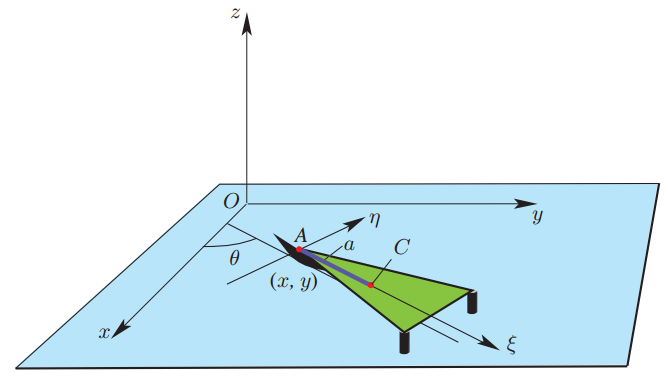
Figure 2. The Chaplygin sleigh

The control inputs are denoted by $u_{1}$ and $u_{2}.$ The first one corresponds to a force applied perpendicular to the center of mass of the sleigh and the second one is the torque applied about the vertical axis.

The constraint is given by the no slip condition and is expressed in differential form by

$$\omega=\sin\theta\,dx-\cos\theta,dy.$$

Therefore the constraint distribution $\mathcal{D}$ is given by

$$\mathcal{D}=\left\{\frac{1}{J}\frac{\partial}{\partial\theta},\frac{\cos\theta}{m}\frac{\partial}{\partial x}+\frac{\sin\theta}{m}\frac{\partial}{\partial y}\right\}.$$

That is, the distribution is given by the span of the vector fields

$$X_{1}(q) = \frac{1}{J}\frac{\partial}{\partial\theta},$$

$$X_{2}(q) = \frac{\cos\theta}{m}\frac{\partial}{\partial x}+\frac{\sin\theta}{m}\frac{\partial}{\partial y}.$$

The Lagrangian is metric on $Q$ where the matrix associated with the metric $\mathcal{G}$ is

$$\mathcal{G}=\left(\begin{array}[]{ccc}m&0&0\\ 0&m&0\\ 0&0&J\\ \end{array}\right).$$

Then the Lagrangian $L:T(\mathds{R}^{2}\times\mathbb{S}^{1})\rightarrow\mathds{R}$ is given by the kinetic energy of the body, which is a sum of the kinetic energy of the center of mass and the kinetic energy due to the rotation of the body

$$L(q,\dot{q})=\frac{m}{2}(\dot{x}_{C}^{2}+\dot{y}_{C}^{2})+\frac{J}{2}\dot{\theta}^{2},$$

where $x_{C}=x+a\cos\theta$,$y_{C}=y+a\sin\theta$.

The projection map $\mathcal{P}:TQ\rightarrow\mathcal{D}$ is

$$\mathcal{P}(q,\dot{q})=\cos^{2}\theta dx\otimes\frac{\partial}{\partial x}+\cos\theta\sin\theta dx\otimes\frac{\partial}{\partial y}+\cos\theta\sin\theta dy\otimes\frac{\partial}{\partial x}+\sin^{2}\theta dy\otimes\frac{\partial}{\partial y}+d\theta\otimes\frac{\partial}{\partial\theta}.$$

Let $q=(x,y,\theta)$ be coordinates on the base manifold $\mathds{R}^{2}\times\mathbb{S}^{1}$ and take the basis $\{X_{1},X_{2}\}$ of vector fields of $\mathcal{D}.$ This basis induces adapted coordinates $(x,y,\theta,y_{1},y_{2})\in\mathcal{D}$ in the following way: Given the vector fields $X_{1}$ and $X_{2}$ generating the distribution we obtain the relations for $q\in\mathds{R}^{2}\times\mathbb{S}^{1}$

$$X_{1}(q) = \rho_{1}^{1}(q)\frac{\partial}{\partial x}+\rho_{1}^{2}(q)\frac{\partial}{\partial y}+\rho_{1}^{3}(q)\frac{\partial}{\partial\theta},$$

$$X_{2}(q) = \rho_{2}^{1}(q)\frac{\partial}{\partial x}+\rho_{2}^{2}(q)\frac{\partial}{\partial y}+\rho_{2}^{3}(q)\frac{\partial}{\partial\theta}.$$

Then,

$$\rho_{1}^{1}=\rho_{1}^{2}=\rho_{2}^{3}=0,\quad\rho_{1}^{3}=\frac{1}{J},\quad\rho_{2}^{1}=\frac{\cos\theta}{m},\quad\rho_{2}^{2}=\frac{\sin\theta}{m}.$$

Each element $e\in{\mathcal{D}}_{q}$ is expressed as a linear combination of these vector fields:

$$e=y_{1}X_{1}(q)+y_{2}X_{2}(q),\quad q\in\mathds{R}^{2}\times\mathbb{S}^{1}.$$

Therefore, the vector subbundle $\tau_{\mathcal{D}}:{\mathcal{D}}\rightarrow\mathds{R}^{2}\times\mathbb{S}^{1}$ is locally described by the coordinates $(x,y,\theta;y_{1},y_{2})$; the first three for the base and the last two, for the fibers. Observe that

$$e=y_{1}\left(\frac{1}{J}\frac{\partial}{\partial\theta}\right)+y_{2}\left(\frac{\cos\theta}{m}\frac{\partial}{\partial x}+\frac{\sin\theta}{m}\frac{\partial}{\partial y}\right)$$

and, in consequence, ${\mathcal{D}}$ is described by the conditions (admissibility conditions):

$$\dot{x}=\frac{\cos\theta}{m}y_{2},\quad\dot{y}=\frac{\sin\theta}{m}y_{2},\quad\dot{\theta}=\frac{1}{J}y_{1}$$

as a vector subbundle of $TQ$ where $y_{1}$ and $y_{2}$ are the adapted velocities relative to the basis of $\mathcal{D}$ defined before.

The nonholonomic bracket given by $[\![\cdot,\cdot]\!]=\mathcal{P}([\cdot,\cdot])$ satisfies

$$[\![X_{1},X_{2}]\!]=\mathcal{P}[X_{1},X_{2}]=\mathcal{P}\left(-\frac{1}{Jm}\sin\theta\frac{\partial}{\partial x}+\frac{\cos\theta}{Jm}\frac{\partial}{\partial y}\right)=0.$$

The restricted Lagrangian function in the new adapted coordinates is given by

$$\ell(x,y,\theta,y_{1},y_{2})=\frac{1}{2m}(y_{2})^{2}+\frac{b}{2J}(y_{1})^{2}\hbox{ where }b=\frac{a^{2}m}{J}.$$

Therefore, the equations of motion are

$$\frac{b\dot{y}_{1}}{J}=0,\quad\frac{\dot{y}_{2}}{m}=0,\quad\dot{x}=\frac{\cos\theta}{m}y_{2},\quad\dot{y}=\frac{\sin\theta}{m}y_{2},\quad\dot{\theta}=\frac{1}{J}y_{1}.$$

Now, by adding controls in our picture, the controlled Euler-Lagrange equations are written as

$$\frac{b\dot{y}_{1}}{J}=u_{2},\quad\frac{\dot{y}_{2}}{m}=u_{1},\quad\dot{x}=\frac{\cos\theta}{m}y_{2},\quad\dot{y}=\frac{\sin\theta}{m}y_{2},\quad\dot{\theta}=\frac{1}{J}y_{1}.$$

The optimal control problem consists on finding an admissible curve satisfying the previous equations given boundary conditions on $\mathcal{D}$ and minimizing the functional $\mathcal{J}(x,y,\theta,y_{1},y_{2},u_{1},u_{2})=\frac{1}{2}\int_{0}^{T}\left(u_{1}^{2}+u_{2}^{2}\right)dt$, for the cost function $C:\mathcal{D}\times U\rightarrow\mathds{R}$ given by

$$C(x,y,\theta,y_{1},y_{2},u_{1},u_{2})=\frac{1}{2}(u_{1}^{2}+u_{2}^{2}).$$ (4)

As before, the optimal control problem is equivalent to solving the constrained optimization problem determined by $\mathcal{L}:\mathcal{D}^{(2)}\rightarrow\mathds{R},$ where

$$\mathcal{L}(x,y,\theta,y_{1},y_{2},\dot{y}_{1},\dot{y}_{2})=\frac{1}{2}\left(\frac{b^{2}\dot{y}_{1}^{2}}{J^{2}}+\frac{\dot{y}_{2}^{2}}{m^{2}}\right).$$

Here, $\mathcal{D}^{(2)}$ is a submanifold of the vector bundle $T\mathcal{D}$ over $\mathcal{D}$ defined by

$$\mathcal{D}^{(2)}:=\left\{(x,y,\theta,y_{1},y_{2},\dot{x},\dot{y},\dot{\theta},\dot{y}_{1},\dot{y}_{2})\in T\mathcal{D}\Big{|}\dot{x}-\frac{\cos\theta}{m}y_{2}=0,\dot{y}-\frac{\sin\theta}{m}y_{2}=0,\dot{\theta}-\frac{1}{J}y_{1}=0\right\},$$

where the inclusion $i_{\mathcal{D}^{(2)}}:\mathcal{D}^{(2)}\hookrightarrow T\mathcal{D},$ is given by the map

$$i_{\mathcal{D}^{(2)}}(x,y,\theta,y_{1},y_{2},\dot{y}_{1},\dot{y}_{2})=\left(x,y,\theta,y_{1},y_{2},\frac{\cos\theta}{m}y_{2},\frac{\sin\theta}{m}y_{2},\frac{1}{J}y_{1},\dot{y}_{1},\dot{y}_{2}\right).$$

The equations of motion for the extended Lagrangian

$$\widetilde{\mathcal{L}}(x,y,\theta,y_{1},y_{2},\dot{x},\dot{y},\dot{\theta},\dot{y}_{1},\dot{y}_{2},\lambda) = \mathcal{L}+\lambda_{1}\left(\dot{x}-\frac{\cos\theta}{m}y_{2}\right)+\lambda_{2}\left(\dot{y}-\frac{\sin\theta}{m}y_{2}\right)$$

$$+\lambda_{3}\left(\dot{\theta}-\frac{1}{J}y_{1}\right)$$

are

$$\dot{\lambda}_{1} = 0,\quad\dot{\lambda}_{2}=0,\quad\dot{\lambda}_{3}=\frac{y_{2}}{m}\left(\lambda_{1}\sin\theta-\lambda_{2}\cos\theta\right),$$

$$\lambda_{3} = -\frac{b^{2}\ddot{y}_{1}}{J},\quad\ddot{y}_{2}=-m(\lambda_{1}\cos\theta+\lambda_{2}\sin\theta)$$

with

$$\dot{x}=\frac{\cos\theta}{m}y_{2},\quad\dot{y}=\frac{\sin\theta}{m}y_{2},\quad\dot{\theta}=\frac{1}{J}y_{1}.$$

The first two equations can be integrated as $\lambda_{1}=c_{1}$ and $\lambda_{2}=c_{2}$ where $c_{1}$ and $c_{2}$ are constants and differentiating the equation for $\lambda_{3}$ with respect to the time and substituting into the third equation, the problem is reduced to solve the system

$$\frac{\dddot{y}_{1}}{J}=\frac{y_{2}}{mb^{2}}\left(c_{2}\cos\theta-c_{1}\sin\theta\right),\quad\ddot{y}_{2}=-m(c_{1}\cos\theta+c_{2}\sin\theta),$$

with

$$\dot{x}=\frac{\cos\theta}{m}y_{2},\quad\dot{y}=\frac{\sin\theta}{m}y_{2},\quad\dot{\theta}=\frac{1}{J}y_{1}.$$

If we suppose, $\lambda_{1}=0,\lambda_{2}=0$ (that is, $c_{1}=c_{2}=0$) then the system can be reduced to solve

$$\dddot{y}_{1}=0\ \hbox{ and }\ \ddot{y}_{2}=0.$$

Integrating these equations and using the admissibility conditions we obtain constants of integration $c_{i},$ $i=3,\ldots,8$ and the equations

$$\theta(t) = \frac{c_{3}t^{3}}{6J}+\frac{c_{4}t^{2}}{2J}+\frac{c_{5}t+c_{6}}{J},$$

$$x(t) = \frac{1}{m}\int_{0}^{t}\cos\left(\frac{c_{3}s^{3}+3c_{4}s^{2}+6c_{5}s+6c_{6}}{6J}\right)\left(c_{7}s+c_{8}\right)ds,$$

$$y(t) = \frac{1}{m}\int_{0}^{t}\sin\left(\frac{c_{3}s^{3}+3c_{4}s^{2}+6c_{5}s+6c_{6}}{6J}\right)\left(c_{7}s+c_{8}\right)ds.$$

Therefore the controls $u_{1}$ and $u_{2}$ are

$$u_{1}(t)=\frac{c_{7}}{m},\quad u_{2}(t)=\frac{c_{3}t+c_{4}}{J}.$$

Remark 3.2.

A similar optimal control problem was studied also [9]. The authors have also used the theory of affine connections to analyze the optimal control problem of underactuated nonholonomic mechanical systems. The main difference with our approach is that in our paper we are working on the distribution $\mathcal{D}$ itself. We impose the extra condition $\lambda_{1}=\lambda_{2}=0$ to obtain explicitlly the controls minimizing the cost function. Usually, there is prescribed an initial boundary condition on $\mathcal{D}$ and a final boundary condition on $\mathcal{D}$. For the Chaplygin sleigh we impose conditions $(x(0),y(0),\theta(0),y_{1}(0),y_{2}(0))$ and $(x(T),y(T),\theta(T),y_{1}(T),y_{2}(T))$. Heuristically, observe that if we transform these conditions into initial conditions we will need to take the initial condition
$(x(0),y(0),\theta(0),y_{1}(0),y_{2}(0),\dot{y}_{1}(0),\dot{y}_{2}(0),\lambda_{1}(0),\lambda_{2}(0),\lambda_{3}(0))$ and it is not necessary that some of the multipliers are zero from the very beginning.

3.3. Application to motion planing for obstacle avoidance: The Chaplygin sleigh with obstacles

In this section, we use the same model of the Chaplygin sleigh from the previous section to show how obstacle avoidance can be achieved with our approach using navigation functions. A navigation function is a potential field-based function used to model an obstacle as a repulsive area or surface [35],[36].

For the Chaplygin sleigh, consider the following boundary conditions on the distribution $\mathcal{D}$: $x(0)=0,\quad y(1)=0,\quad\theta(0)=0,\quad y_{1}(0)=0,\quad y_{2}(0)=0$ and $x(T)=1,\quad y(T)=1,\quad\theta(T)=0,\quad y_{1}(T)=0,\quad y_{2}(T)=0.$

Let the obstacle be circular in the $xy$-plane, located at the point $(x_{C},y_{C})=(0.5,0.5)$. For llustrative purposes, we use a simple inverse square law for the navigation function. Let $V(x,y)$ given by

$$V(x,y)=\frac{\kappa}{(x-x_{C})^{2}+(y-y_{C})^{2}}$$

where the parameter $\kappa$ is introduced to control the strength of the potential function.

Appending the potential into the cost functional (4) the optimal control problem is equivalent to solve the constrained optimization problem determined by $\mathcal{L}:\mathcal{D}^{(2)}\rightarrow\mathds{R},$ where

$$\mathcal{L}(x,y,\theta,y_{1},y_{2},\dot{y}_{1},\dot{y}_{2})=\frac{b^{2}\dot{y}_{1}^{2}}{2J^{2}}+\frac{\dot{y}_{2}^{2}}{2m^{2}}+\frac{\kappa}{2((x-x_{C})^{2}+(y-y_{C})^{2})}.$$

The equations of motion for the extended Lagrangian

$$\widetilde{\mathcal{L}}(x,y,\theta,y_{1},y_{2},\dot{x},\dot{y},\dot{\theta},\dot{y}_{1},\dot{y}_{2},\lambda) = \mathcal{L}+\lambda_{1}\left(\dot{x}-\frac{\cos\theta}{m}y_{2}\right)+\lambda_{2}\left(\dot{y}-\frac{\sin\theta}{m}y_{2}\right)$$

$$+\lambda_{3}\left(\dot{\theta}-\frac{1}{J}y_{1}\right)$$

are

$$\dot{\lambda}_{1} = -\frac{\kappa(x-x_{C})}{((x-x_{C})^{2}+(y-y_{C})^{2})^{2}}\quad\dot{\lambda}_{2}=-\frac{\kappa(y-y_{C})}{((x-x_{C})^{2}+(y-y_{C})^{2})^{2}},$$

$$\dot{\lambda}_{3} = \frac{y_{2}}{m}\left(\lambda_{1}\sin\theta-\lambda_{2}\cos\theta\right),\quad\lambda_{3}=-\frac{b^{2}\ddot{y}_{1}}{J},\quad\ddot{y}_{2}=-m(\lambda_{1}\cos\theta+\lambda_{2}\sin\theta)$$

with

$$\dot{x}=\frac{\cos\theta}{m}y_{2},\quad\dot{y}=\frac{\sin\theta}{m}y_{2},\quad\dot{\theta}=\frac{1}{J}y_{1}.$$

We solve the earlier boundary value problem for several values of $\kappa$. Starting with $\kappa=0$, which corresponds to a zero potential function, we incremente $\kappa$ until the potential field was strong enough to prevent the sleigh from interfering with the obstacle. We try with $\kappa=0,0.01,0.1,0.25,$ and $0.5$ for $T$=1. The result is shown in Fig. $4$. Note that for $\kappa=0.25$ and $0.5$ the sleigh avoids the obstacle, and as one may anticipate, as $\kappa$ increases, the total control effort and therefore, the total cost $\displaystyle{\mathcal{J}=\frac{1}{2}\int_{0}^{1}(u_{1}^{2}+u_{2}^{2}+V(x,y))dt}$ increases. For example, $\mathcal{J}=17.0242$ when $\kappa=0.25$ and $\mathcal{J}=18.4634$ when $\kappa=0.5$. Hence, we select $\kappa=0.25$ since it corresponds to a trajectory that avoids the obstacle with the least possible cost (of all five tried in this simulation). The trajectories profile is shown in Figures $5$, $6$ and $7$. This example illustrate how our approach can be used with the method of navigation functions of optimal motion generation for obstacle avoidance.

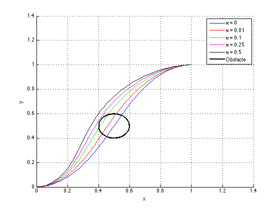
Figure 3. The extremals solving the boundary value problem with $\kappa=0,0.01,0.1,0.25$ and $0.5$.

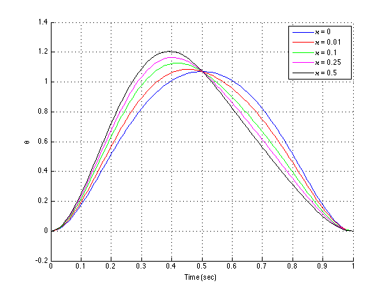
Figure 4. Behavior of $\theta$ for $\kappa=0,0.01,0.1,0.25$ and $0.5$.

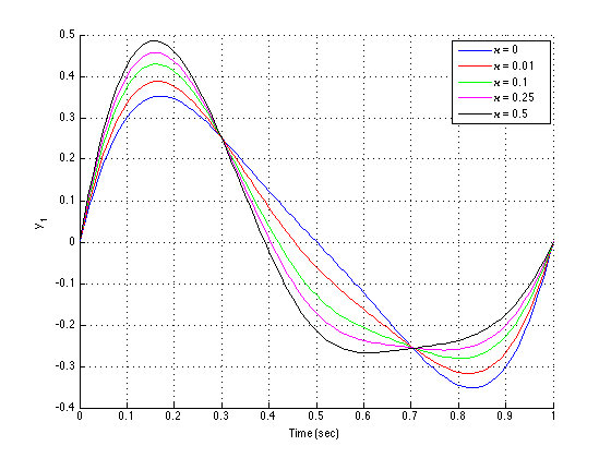
Figure 5. Behavior of the velocites $y_{1}$ (left) and $y_{2}$ (right) for $\kappa=0,0.01,0.1,0.25$ and $0.5$

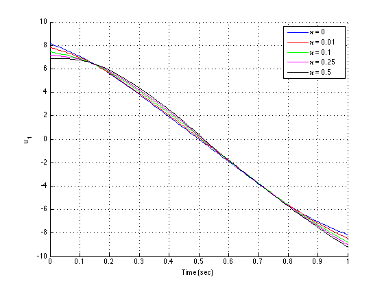
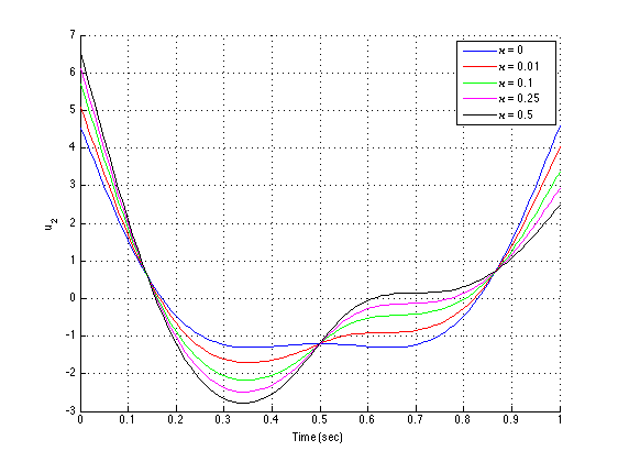
Figure 6. Behavior of the controls $u_{1}$ (left) and $u_{2}$ (right) for $\kappa=0,0.01,0.1,0.25$ and $0.5$

4. Lagrangian submanifolds and nonholonomic optimal control problems

In this section we study the construction of Lagrangian submanifold representing intrinsically the dynamics of the optimal control problem and the corresponding Hamiltonian representation when the system is regular. In the regular case, the definition of a particular Legendre transformation give rise the relationship and correspondence between the Lagrangian and Hamiltonian dynamics.

4.1. Lagrangian submanifolds

In this subsection we will construct Lagrangian submanifolds that are interesting for our purposes in the study of the geometry of optimal control problems of controlled mechanical systems (see [33, 49]).

Definition 4.1.

Given a finite-dimensional symplectic manifold $(P,\omega)$ and a submanifold $N$, with canonical inclusion $i_{N}:N\hookrightarrow P$, $N$ is said to be a Lagrangian submanifold if $i^{*}_{N}\,\omega=0$ and

$$\mbox{dim}\hskip 2.84526ptN=\frac{1}{2}\mbox{dim}\hskip 2.84526ptP.$$

A distinguished symplectic manifold is the cotangent bundle $T^{*}Q$ of any manifold $Q$. If we choose local coordinates $(q^{i})$, $1\leq i\leq n$, then $T^{*}Q$ has induced coordinates $(q^{i},p_{i})$. Denote by $\pi_{Q}:T^{*}Q\to Q$ the canonical projection of the cotangent bundle defined by $\pi_{Q}(\epsilon_{q})=q$, where $\epsilon_{q}\in T^{*}_{q}Q$. Define the Liouville 1-form or canonical 1-form $\theta_{Q}\in\Lambda^{1}(T^{*}Q)$ by

$$\langle(\theta_{Q})_{\epsilon}\,,\,X\rangle=\langle\epsilon\,,\,T\pi_{Q}(X)\rangle,\hbox{ where }X\in T_{\epsilon}T^{*}Q\;,\ \epsilon\in T^{*}Q.$$

In local coordinates we have that $\theta_{Q}=p_{i}\,\mathrm{d}q^{i}$. The canonical two-form $\omega_{Q}$ on $T^{*}Q$ is the symplectic form $\omega_{Q}=-\mathrm{d}\theta_{Q}$ (that is $\omega_{Q}=\mathrm{d}q^{i}\wedge\mathrm{d}p_{i}$).

Now, we will introduce some special Lagrangian submanifolds of the symplectic manifold $(T^{*}Q,\omega_{Q})$. For instance, the image ${\Sigma}_{\lambda}=\lambda(Q)\subset T^{*}Q$ of a closed 1-form $\lambda\in\Lambda^{1}Q$ is a Lagrangian submanifold of $(T^{*}Q,\omega_{Q})$, since $\lambda^{*}\omega_{Q}=-\mathrm{d}\lambda=0$. We then obtain a submanifold diffeomorphic to $Q$ and transverse to the fibers of $T^{*}Q$. When $\lambda$ is exact, that is, $\lambda=\mathrm{d}f$, where $f:Q\to\mathds{R}$, we say that $f$ is a generating function of the Lagrangian submanifold ${\Sigma}_{\lambda}=\Sigma_{f}$ (see [49]).

A useful extension of the previous construction is the following result due to W.Tulczyjew:

Theorem 4.1 ([47],[48]).

Let $Q$ be a smooth manifold, $\tau_{Q}:TQ\rightarrow Q$ its tangent bundle projection, $N\subset Q$ a submanifold, and $f\colon N\rightarrow\mathbb{R}$. Then

$$\Sigma_{f}=\bigl{\{}p\in T^{\ast}Q\mid\pi_{Q}(p)\in N\text{ and }\left\langle p,v\right\rangle=\left\langle\mathrm{d}f,v\right\rangle\\ \text{ for all }v\in TN\subset TQ\text{ such that }\tau_{Q}(v)=\pi_{Q}(p)\bigr{\}}$$

is a Lagrangian submanifold of $T^{\ast}Q$.

Taking $f$ as the zero function, for example, we obtain the following Lagrangian submanifold

$$\Sigma_{0}=\left\{p\in T^{*}Q\big{|}_{N}\,|\,\langle p\,,\,v\rangle=0\,,\,\forall\,v\in TN\,\mbox{ with }\,\tau_{Q}(v)=\pi_{Q}(p)\right\},$$

which is just the conormal bundle of $N$:

$$\nu^{*}(N)=\left\{p\in T^{*}Q\big{|}_{N}\,;\,p\big{|}_{T_{\pi(p)}N}=0\right\}.$$

4.2. Lagrangian submanifold description of nonholonomic mechanical control problems

Next, we derive the equations of motion representing the dynamics of the optimal control problem .

Given the function $\mathcal{L}:\mathcal{D}^{(2)}\rightarrow\mathds{R},$ following Theorem (4.1), when $N=\mathcal{D}^{2}\subset T{\mathcal{D}}$ we have the Lagrangian submanifold $\Sigma_{\mathcal{L}}\subset T^{*}T\mathcal{D}.$ Therefore, $\mathcal{L}:\mathcal{D}^{(2)}\rightarrow\mathbb{R}$ generates a Lagrangian submanifold $\Sigma_{\mathcal{L}}\subset T^{*}T\mathcal{D}$ of the symplectic manifold $(T^{*}T\mathcal{D},\omega_{T\mathcal{D}})$ where $\omega_{T\mathcal{D}}$ is the canonical symplectic 2-form on $T^{*}T\mathcal{D}.$

The relationship between these spaces is summarized in the following diagram:

Proposition 4.1.

Let $\mathcal{L}:\mathcal{D}^{(2)}\rightarrow\mathbb{R}$ be a $C^{\infty}$-function. Consider the inclusion $i_{\mathcal{D}^{(2)}}:\mathcal{D}^{(2)}\rightarrow T\mathcal{D}$ where $\omega_{T\mathcal{D}}$ is the canonical symplectic 2-form in $T^{*}T\mathcal{D}.$ Then

$$\Sigma_{\mathcal{L}}=\{\mu\in T^{*}T\mathcal{D}|i_{\Sigma_{\mathcal{L}}}^{*}\mu=d\mathcal{L}\}\subset T^{*}T\mathcal{D}$$

is a Lagrangian submanifold of $(T^{*}T\mathcal{D},\omega_{T\mathcal{D}}).$

Definition 4.2.

Let $\mathcal{D}$ be a non-integrable distribution, $T\mathcal{D}$ its tangent bundle and $\mathcal{D}^{(2)}$ the subbundle of $T\mathcal{D}$ defined on (1). A second-order nonholonomic system is a pair $(\mathcal{D}^{(2)},\Sigma_{\mathcal{L}})$ where $\Sigma_{\mathcal{L}}\subset T^{*}T\mathcal{D}$ is the Lagrangian submanifold generated by $\mathcal{L}:\mathcal{D}^{(2)}\rightarrow\mathds{R}.$

Consider local coordinates $(q^{i},y^{A},\dot{q}^{i},\dot{y}^{A})$ on $T\mathcal{D}.$ These coordinates induce local coordinates $(q^{i},y^{A},\dot{q}^{i},\dot{y}^{A},\mu_{i},\mu_{A},\gamma_{i},\gamma_{A})$ on $T^{*}T\mathcal{D}.$ Therefore, locally, the system is characterized by the following set of equations on $T^{*}T\mathcal{D}$

$$\mu_{i}+\gamma_{j}\frac{\partial\rho_{A}^{j}}{\partial q^{i}}y^{A} = \frac{\partial\mathcal{L}}{\partial q^{i}},$$

$$\mu_{A}+\gamma_{j}\rho_{A}^{j} = \frac{\partial\mathcal{L}}{\partial y^{A}},$$ (5)

$$\gamma_{A} = \frac{\partial\mathcal{L}}{\partial\dot{y}^{A}},$$

$$\dot{q}^{i} = \rho_{A}^{i}y^{A}.$$

Remark 4.3.

Typically local coordinates on $\Sigma_{\mathcal{L}}\subset T^{*}T\mathcal{D}$ are $(q^{i},y^{A},\dot{y}^{A},\gamma_{i})$ where $\gamma_{i}$ plays the role of Lagrange multipliers.

Remark 4.4.

In the case of the Chaplygin sleigh local coordinates on $T^{*}T\mathcal{D}$ will be given by $(x,y,\theta,y_{1},y_{2},\dot{x},\dot{y},\dot{\theta},\dot{y}_{1},\dot{y}_{2},\mu_{x},\mu_{y},\mu_{\theta},\mu_{1},\mu_{2},\gamma_{x},\gamma_{y},\gamma_{\theta},\gamma_{1},\gamma_{2})$, where $(x,y,\theta,y_{1},y_{2},\dot{x},\dot{y},\dot{\theta},\dot{y}_{1},\dot{y}_{2})$ are local coordinates on $T\mathcal{D}$. The Lagrangian submanifold of $T^{*}T\mathcal{D}$ is described by the equations

$$\mu_{x} = 0,\quad\mu_{y}=0,$$

$$\mu_{\theta} = \frac{y_{2}}{m}\left(\gamma_{x}\sin\theta-\gamma_{y}\cos\theta\right),$$

$$\mu_{1} = -\frac{b^{2}\gamma_{\theta}}{J},\quad\mu_{2}=-m(\gamma_{x}\cos\theta+\gamma_{y}\cos\theta),$$

$$\gamma_{1} = \frac{b^{2}\dot{y}_{1}}{J^{2}},\quad\gamma_{2}=\frac{\dot{y}_{2}}{m^{2}},$$

$$\dot{x} = \frac{\cos\theta}{m}y_{2},\quad\dot{y}=\frac{\sin\theta}{m}y_{2},\quad\dot{\theta}=\frac{y_{1}}{J}.$$

After a straightforward computation one can check easily that these equations are equivalent with those obtained in the Lagrangian formalism.

4.3. Legendre transformation and regularity condition

We define the map $\Psi:T^{*}T\mathcal{D}\rightarrow T^{*}\mathcal{D}$ as

$$\langle\Psi(\mu_{v_{x}}),X(x)\rangle=\langle\mu_{v_{x}},X^{V}(v_{x})\rangle,$$

where $\mu\in T^{*}T\mathcal{D},v_{x}\in T_{x}\mathcal{D},$ $X(x)\in T_{x}\mathcal{D}$ and $X^{V}(v_{x})\in T_{v_{x}}T\mathcal{D}$ is its vertical lift to $v_{x}.$ Locally,

$$\Psi(q^{i},y^{A},\dot{q}^{i},\dot{y}^{A},\mu_{i},\mu_{A},\gamma_{i},\gamma_{A})=(q^{i},y^{A},\gamma_{i},\gamma_{A}).$$

Definition 4.5.

Define the Legendre transform associated with a second-order nonholonomic system $(\mathcal{D}^{(2)},\Sigma_{\mathcal{L}})$ as the map $\mathbb{F}\mathcal{L}:\Sigma_{\mathcal{L}}\rightarrow T^{*}\mathcal{D}$ given by $\mathbb{F}\mathcal{L}=\Psi\circ i_{\Sigma_{\mathcal{L}}}.$ In local coordinates, it is given by

$$\mathbb{F}\mathcal{L}(q^{i},y^{A},\dot{y}^{A},\gamma_{i})=\left(q^{i},y^{A},\gamma_{i},\frac{\partial\mathcal{L}}{\partial\dot{y}^{A}}\right).$$

The following diagram summarizes the situation

Definition 4.6.

We say that the second-order nonholonomic system $(\mathcal{D}^{(2)},\Sigma_{\mathcal{L}})$ is regular if $\mathbb{F}\mathcal{L}:\Sigma_{\mathcal{L}}\rightarrow T^{*}\mathcal{D}$ is a local diffeomorphism and hyperregular if $\mathbb{F}\mathcal{L}$ is a global diffeomorphism.

From the local expression of $\mathbb{F}\mathcal{L}$ we can observe that from a direct application of the implicit function theorem we have:

Proposition 4.2.

The second-order nonholonomic system $(\mathcal{D}^{(2)},\Sigma_{\mathcal{L}})$ determined by $\mathcal{L}:\mathcal{D}^{(2)}\rightarrow\mathds{R}$ is regular if and only if the matrix $\displaystyle{\left(\frac{\partial^{2}\mathcal{L}}{\partial\dot{y}^{A}\partial\dot{y}^{B}}\right)}$ is non singular.

Remark 4.7.

Observe that if the Lagrangian $\mathcal{L}:\mathcal{D}^{(2)}\rightarrow\mathds{R}$ is determined from an optimal control problem and its expression is given by (2) then the regularity of the matrix $\displaystyle{\left(\frac{\partial^{2}\mathcal{L}}{\partial\dot{y}^{A}\partial\dot{y}^{B}}\right)}$ is equivalent to

$$\det\left(\frac{\partial^{2}C}{\partial u^{A}\partial u^{B}}\right)\neq 0$$

for the cost function.

4.4. Hamiltonian formalism

Assume that the system is regular. Then if we denote by $p_{i}=\gamma_{i}$ and $\displaystyle{p_{A}=\frac{\partial\mathcal{L}}{\partial\dot{y}^{A}}}$ we can write $\dot{y}^{A}=\dot{y}^{A}(q^{i},y^{A},p_{A}).$ Define the Hamiltonian function $\mathcal{H}:T^{*}\mathcal{D}\rightarrow\mathds{R}$ by

$$\mathcal{H}(\alpha)=\langle\alpha,\pi_{T^{*}T\mathcal{D}}\mid_{\Sigma_{\mathcal{L}}}\left(\mathbb{F}\mathcal{L}^{-1}(\alpha)\right)\rangle-\mathcal{L}\left(\pi_{T^{*}T\mathcal{D}}\mid_{\Sigma_{\mathcal{L}}}\left(\mathbb{F}\mathcal{L}^{-1}(\alpha)\right)\right)$$

where $\alpha\in T^{*}\mathcal{D}$ is a one-form on $\mathcal{D},$ and $\pi_{T^{*}T\mathcal{D}}\mid_{\Sigma_{\mathcal{L}}}:\Sigma_{\mathcal{L}}\rightarrow\mathcal{D}^{(2)}$ is the projection locally given by $\pi_{T^{*}T\mathcal{D}}\mid_{\Sigma_{\mathcal{L}}}(q^{i},y^{A},\dot{y}^{A},\gamma_{i})=(q^{i},y^{A},\dot{y}^{A}).$ Locally the Hamiltonian is given by

$$\mathcal{H}(q^{i},y^{A},p_{i},p_{A})=p_{A}\dot{y}^{A}(q^{i},y^{A},p_{A}))+p_{i}\rho_{A}^{i}y^{A}-\mathcal{L}(q^{i},y^{A},\dot{y}^{A}(q^{i},y^{A},p_{A})),$$

where we are using

$$\mathbb{F}\mathcal{L}^{-1}(q^{i},y^{A},p_{i},p_{A})=\left(q^{i},y^{A},\rho_{A}^{i},\dot{y}^{A}(q^{i},y^{A},p_{A}),\frac{\partial\mathcal{L}}{\partial q^{i}}-p_{j}\frac{\partial\rho_{A}^{j}}{\partial q^{i}}y^{A},\frac{\partial\mathcal{L}}{\partial y^{A}}-p_{j}\rho_{A}^{j},p_{i},p_{A}\right).$$

Below we will see that the dynamics of the nonholonomic optimal control problem is determined by the Hamiltonian system given by the triple $(T^{*}\mathcal{D},\omega_{\mathcal{D}},\mathcal{H})$ where $\omega_{\mathcal{D}}$ is the standard symplectic $2-$form on $T^{*}\mathcal{D}.$

The dynamics of the optimal control problem for the second-order nonholonomic system is given by the symplectic hamiltonian dynamics determined by the dynamical equation

$$i_{X_{\mathcal{H}}}\omega_{\mathcal{D}}=d\mathcal{H}.$$ (6)

Therefore, if we consider the integral curves of $X_{\mathcal{H}},$ there are of the type $t\mapsto(\dot{q}^{i}(t),\dot{y}^{A}(t),\dot{p}_{i}(t),\dot{p}_{A}(t));$ the solutions of the nonholonomic Hamiltonian system is specified by the Hamilton’s equations on $T^{*}\mathcal{D}$

$$\dot{q}^{i} = \frac{\partial\mathcal{H}}{\partial p_{i}},\qquad\quad\dot{y}^{A}=\frac{\partial\mathcal{H}}{\partial p_{A}},$$

$$\dot{p}_{i} = -\frac{\partial\mathcal{H}}{\partial q^{i}},\qquad\dot{p}_{A}=-\frac{\partial\mathcal{H}}{\partial y^{A}};$$

that is,

$$\dot{q}^{i} = \rho_{A}^{i}y^{A},$$

$$\dot{p}_{i} = \frac{\partial\mathcal{L}}{\partial q^{i}}(q^{i},y^{A},\dot{y}^{A}(q^{i},y^{A},p_{A}))-p_{j}\frac{\partial\rho_{A}^{j}}{\partial q^{i}}y^{A},$$

$$\dot{p}_{A} = \frac{\partial\mathcal{L}}{\partial y^{A}}(q^{i},y^{A},\dot{y}^{A}(q^{i},y^{A},p_{A}))-p_{j}\rho_{A}^{j}.$$

From equation (6) it is clear that the flow preserves the symplectic $2-$form $\omega_{\mathcal{D}}.$ Moreover, these equations are equivalent to equations given in (3) using the identification between the Lagrange multipliers with the variables $p_{i}$ and the relation for $\displaystyle{p_{A}}=\frac{\partial\mathcal{L}}{\partial\dot{y}^{A}}.$

Remark 4.8.

We observe that in our formalism the optimal control dynamics is deduced using a constrained variational procedure and equivalently it is possible to apply the Hamilton-Pontryagin’s principle (see [21] for example), but, in any case, this “variational procedure” implies the preservation of the symplectic 2-form, and this is reflected in the Lagrangian submanifold character. Moreover, in our case, under the regularity condition, we have seen that the Lagrangian submanifold shows that the system can be written as a Hamiltonian system (which is obviously symplectic).

Additionally, we use the Lagrangian submanifold $\Sigma_{\mathcal{L}}$ as a way to define intrinsically the Hamiltonian side since we define the Legendre transformation using the Lagrange submanifold $\Sigma_{\mathcal{L}}$. However there exist other possibilities. For instance, in [1] (Section 4.2) the authors defined the corresponding momenta for a vakonomic system. Using this procedure the momenta are locally expressed as follows

$$p_{i} = \frac{\partial\widetilde{\mathcal{L}}}{\partial\dot{q}^{i}}+\lambda^{j}\frac{\partial f_{j}}{\partial\dot{q}^{i}}$$

$$p_{A} = \frac{\partial\widetilde{\mathcal{L}}}{\partial\dot{y}^{A}}+\lambda^{j}\frac{\partial f^{j}}{\partial\dot{y}^{A}}$$

where $\widetilde{\mathcal{L}}$ is an arbitrary extension of ${\mathcal{L}}$ to $T{\mathcal{D}}$ and $f^{j}=\dot{q}^{j}-\rho^{j}_{A}y^{A}=0$ are the constraint equations. A simple computation shows that both are equivalent, but our derivation is more intrinsic and geometric, that is, independent of coordinates or extensions and without using Lagrange multipliers.

4.5. Example: continuously variable transmission (CVT) (cont’d)

Now, we continue the example of the optimal control problem for a continuously variable transmission that we considered in Section $3.1$. Recall that the constraint distribution for the CVT is given by $\mathcal{D}\subset T(\mathbb{S}^{1}\times\mathbb{S}^{1}\times\mathds{R})$

$$\mathcal{D}=\left\{\frac{1}{m}\frac{\partial}{\partial x},(1-x)\frac{\partial}{\partial\theta_{1}}+x\frac{\partial}{\partial\theta_{2}}\right\}.$$

The system is regular since

$$\det\left(\frac{\partial^{2}\mathcal{L}}{\partial\dot{y}^{A}\partial\dot{y}^{B}}\right)=\frac{(B(x))^{2}}{m^{2}}\neq 0$$

since $B(x)=J_{1}(1-x)^{2}+J_{2}x^{2}\neq 0$.

Denoting by $(\theta_{1},\theta_{2},x,y_{1},y_{2},p_{\theta_{1}},p_{\theta_{2}},p_{x},p_{1},p_{2})$ local coordinates on $T^{*}\mathcal{D}$ the dynamic of the optimal control problem for this nonholonomic system is determined by the Hamiltonian function $\mathcal{H}:T^{*}\mathcal{D}\rightarrow\mathds{R},$

$$\mathcal{H}(\theta,\theta_{2},x,y_{1},y_{2},p_{\theta_{1}},p_{\theta_{2}},p_{x},p_{1},p_{2}) = \frac{m^{2}p_{1}^{2}}{2}+\frac{p_{2}^{2}}{2(B(x))^{2}}+\frac{p_{2}A(x)y_{1}y_{2}}{mB(x)}+p_{\theta_{1}}(1-x)y_{2}$$

$$+ p_{\theta_{2}}xy_{2}+p_{x}\frac{y_{1}}{m}.$$

The corresponding Hamiltonian equations of motion are

$$\dot{y}_{1} = m^{2}p_{1},\quad\dot{p}_{\theta_{1}}=0,$$

$$\dot{y}_{2} = \frac{p_{2}}{(B(x))^{2}}+\frac{A(x)y_{1}y_{2}}{mB(x)},\quad\dot{p}_{\theta_{2}}=0,$$

$$\dot{p}_{x} = y_{2}(p_{\theta_{1}}-p_{\theta_{2}})-\frac{p_{2}y_{1}y_{2}((A(x))^{2}-J_{1}J_{2})}{m(B(x))^{2}}-\frac{2p_{2}^{2}A(x)}{(B(x))^{3}},$$

$$\dot{p}_{1} = =-\frac{p_{2}A(x)y_{2}}{mB(x)}-\frac{p_{x}}{m},\quad\dot{p}_{2}=-\frac{p_{2}A(x)y_{1}}{mB(x)}-p_{\theta_{1}}(1-x)-p_{\theta_{2}}x.$$

4.6. Example: the Chaplygin sleigh (cont’d)

In what follows, we continue the example of the optimal control problem of the Chaplygin sleigh that we began to study in Section $3.2$. Recall that the constraint distribution is given by $\mathcal{D}\subset TSE(2)$ where

$$\mathcal{D}=\left\{\frac{1}{J}\frac{\partial}{\partial\theta},\frac{\cos\theta}{m}\frac{\partial}{\partial x}+\frac{\sin\theta}{m}\frac{\partial}{\partial y}\right\}.$$

The system is regular since

$$\det\left(\frac{\partial^{2}\mathcal{L}}{\partial\dot{y}^{A}\partial\dot{y}^{B}}\right)=\frac{a^{4}}{J^{4}}\neq 0.$$

Denoting by $(x,y,\theta,y_{1},y_{2},p_{x},p_{y},p_{\theta},p_{1},p_{2})$ local coordinates on $T^{*}\mathcal{D}$ the dynamics of the optimal control problem for this nonholonomic system is determined by the Hamiltonian function $\mathcal{H}:T^{*}\mathcal{D}\rightarrow\mathds{R},$

$$\mathcal{H}(x,y,\theta,y_{1},y_{2},p_{x},p_{y},p_{\theta},p_{1},p_{2})=\frac{J^{2}}{2b^{2}}p_{1}^{2}+\frac{m^{2}}{2}p_{2}^{2}+p_{x}\frac{\cos\theta}{m}y_{2}+\frac{p_{\theta}}{J}y_{1}+p_{y}\frac{\sin\theta}{m}y_{2}.$$

The Hamiltonian equations of motion are

$$\dot{y}_{1} = \frac{J^{2}p_{1}}{b^{2}},\quad\dot{y}_{2}=m^{2}p_{2},\quad\dot{p}_{x}=0,\quad\dot{p}_{y}=0,$$

$$\dot{p}_{\theta} = p_{x}\frac{\sin\theta}{m}y_{2}-p_{y}\frac{\cos\theta}{m}y_{2},$$

$$\dot{p}_{1} = =-\frac{p_{\theta}}{J},\quad\dot{p}_{2}=-p_{x}\frac{\cos\theta}{m}-p_{y}\frac{\sin\theta}{m}.$$

Integrating the equations $\dot{p}_{x}=0$ and $\dot{p}_{y}=0$ as $p_{x}=c_{1}$ and $p_{y}=c_{2}$ where $c_{1}$ and $c_{2}$ are constants the system of differential equations becomes

$$\dot{y}_{1} = \frac{J^{2}p_{1}}{b^{2}},\quad\dot{p}_{\theta}=c_{1}\frac{\sin\theta}{m}y_{2}-c_{2}\frac{\cos\theta}{m}y_{2},$$

$$\dot{y}_{2} = m^{2}p_{2},\quad\dot{p}_{1}=-\frac{p_{\theta}}{J},\quad\dot{p}_{2}=-c_{1}\frac{\cos\theta}{m}-c_{2}\frac{\sin\theta}{m}.$$

Differentiating $\dot{y}_{1}$ and $\dot{y}_{2}$ and substituting we obtain

$$\frac{\dddot{y}_{1}}{J}=\frac{y_{2}}{mb^{2}}\left(c_{2}\cos\theta-c_{1}\sin\theta\right),\quad\ddot{y}_{2}=-m(c_{1}\cos\theta+c_{2}\sin\theta),$$

as in the Lagrangian setting.

Observe that in the case of motion planing for obstacle avoidance the Hamiltonian function $\mathcal{H}:T^{*}\mathcal{D}\to\mathds{R}$ is given by

$$\mathcal{H}(x,y,\theta,y_{1},y_{2},p_{x},p_{y},p_{\theta},p_{1},p_{2}) = \frac{J^{2}}{2b^{2}}p_{1}^{2}+\frac{m^{2}}{2}p_{2}^{2}+p_{x}\frac{\cos\theta}{m}y_{2}+\frac{p_{\theta}}{J}y_{1}+p_{y}\frac{\sin\theta}{m}y_{2}$$

$$- \frac{\kappa}{2(x-x_{C})^{2}+2(y-y_{C})^{2}},$$

and the resulting dynamical equations are

$$\dot{y}_{1} = \frac{J^{2}p_{1}}{b^{2}},\quad\dot{y}_{2}=m^{2}p_{2}\;,\quad\dot{p}_{x}=\frac{\kappa(x-x_{C})}{((x-x_{C})^{2}+(y-y_{C})^{2})^{2}},$$

$$\dot{p}_{y} = \frac{\kappa(y-y_{C})}{((x-x_{C})^{2}+(y-y_{C})^{2})^{2}}\;,\quad\dot{p}_{\theta}=p_{x}\frac{\sin\theta}{m}y_{2}-p_{y}\frac{\cos\theta}{m}y_{2},$$

$$\dot{p}_{1} = =-\frac{p_{\theta}}{J},\quad\dot{p}_{2}=-p_{x}\frac{\cos\theta}{m}-p_{y}\frac{\sin\theta}{m}.$$

5. Conclusions and future research

In this section we summarize the contributions of our work and discuss future research.

5.1. Conclusions:

In this paper we study optimal control problems for a class of nonholonomic mechanical systems. We have given a geometrical derivation of the equations of motion of a nonholonomic optimal control problem as a constrained problem on the tangent space to the constraint distribution. We have seen how the dynamics of the optimal control problem can be completely described by a Lagrangian submanifold of an appropriate cotangent bundle and under some mild regularity conditions we have derived the the equations of motion for the nonholonomic optimal control problem as a classical set of Hamilton’s equations on the cotangent bundle of the constraint distribution. We have introduced the notion of Legendre transformation in this context to establish the relationship between the Lagrangian and Hamiltonian dynamics. We applied our techniques to different examples: optimal control of a continuously variable transmission, Chaplygin sleigh and to optimal planning for obstacle avoidance problems.

5.2. Future research: Construction of geometric and variational integrators for optimal control problems of nonholonomic mechanical systems.

In this paper we have seen that an optimal control problem of a nonholonomic system may be viewed as a Hamiltonian system on $T^{*}\mathcal{D}$. One can thus use standard methods for symplectic integration such as symplectic Runge-Kutta methods, collocation methods, St$\ddot{\hbox{o}}$rmer-Verlet, symplectic Euler methods, etc.; developed and studied in [26], [27], [28], [43], [44], e.g., to simulate nonholonomic optimal control problems.

Also, we would like to build variational integrators as an alternative way to construct integration schemes for these kinds of optimal control problems following the results given in Section 3. Recall that in the continuous case we have considered a Lagrangian function $\mathcal{L}:\mathcal{D}^{(2)}\to\mathds{R}$. Since the space $\mathcal{D}^{(2)}$ is a subset of $T\mathcal{D}$ we can discretize the tangent bundle $T\mathcal{D}$ by the cartesian product $\mathcal{D}\times\mathcal{D}$. Therefore, our discrete variational approach for optimal control problems of nonholonomic mechanical systems will be determined by the construction of a discrete Lagrangian $\mathcal{L}_{d}:\mathcal{D}_{d}^{(2)}\to\mathds{R}$ where $\mathcal{D}^{(2)}_{d}$ is the subset of $\mathcal{D}\times\mathcal{D}$ locally determined by imposing the discretization of the constraint $\dot{q}^{i}=\rho_{A}^{i}(q)y^{A}$, for instance we can consider

$$\mathcal{D}_{d}^{(2)}=\left\{(q_{0}^{i},y_{0}^{A},q_{1}^{i},y^{A}_{1})\in\mathcal{D}\times\mathcal{D}\bigg{|}\frac{q_{1}^{i}-q_{0}^{i}}{h}=\rho_{A}^{i}\left(\frac{q_{0}^{i}+q_{0}^{i}}{2}\right)\left(\frac{y_{0}^{A}+y_{1}^{A}}{2}\right)\right\}.$$

Now the system is in a form appropriate for the application of discrete variational methods for constrained systems (see [34] and references therein).

Acknowledgment

We wish to thanks Klas Modin and Olivier Verdier the permission to use their graphical illustration and description of the Continuously Variable Transmission Gearbox.

References

• [1] Arnold V. Dynamical Systems, Vol. III, Springer-Verlag, New York, Heidelberg, Berlin, (1988).
• [2] Balseiro P, de León M, Marrero J.C and Martín de Diego D. The ubiquity of the symplectic Hamiltonian equations in mechanics. J. Geom. Mech. 1 (2009), 11–34.
• [3] Barbero Liñan M, de León M, Marrero JC, Martín de Diego D and Muñoz Lecanda M. Kinematic reduction and the Hamilton-Jacobi equation. J. Geometric Mechanics, , Issue 3 (2012), 207–237.
• [4] Bloch A.M, Nonholonomic Mechanics and Control. Interdisciplinary Applied Mathematics Series, 24, Springer-Verlag, New York (2003).
• [5] Bloch A and Crouch P. Nonholonomic and vakonomic control systems on Riemannian manifolds, in Dynamics and Control of Mechanical Systems, Michael J. Enos, ed., Fields Inst. Commun. 1, AMS, Providence, RI, 1993, 25–52.
• [6] Bloch A and Crouch P. Nonholonomic control systems on Riemannian manifolds, SIAM J. Control Optim., 33 (1995), 126–148.
• [7] Bloch A and Crouch P. On the equivalence of higher order variational problems and optimal control problems, in Proceedings of the IEEE International Conference on Decision and Control, Kobe, Japan, 1996, 1648–1653.
• [8] Bloch A and Crouch P. Optimal Control, Optimization, and Analytical Mechanics, in Mathematical Control Theory, J. Baillieul and J.C. Willems, eds., Springer-Verlag, New York, 1998, pp. 268–321.
• [9] Bloch A and Hussein I, Optimal Control of Underactuated Nonholonomic Mechanical Systems, IEEE Transactions on Automatic Control 53, (2008) 668–682.
• [10] Bloch A, Marsden J, Zenkov D. Nonholonomic Mechanics, Notices of the AMS 52, (2005), 324?333.
• [11] Bloch A, Marsden J and Zenkov D. Quasivelocities and symmetries in non-holonomic systems. Dynamical Systems, 24 (2), (2009), 187–222.
• [12] Borisov A and Mamaev I. On the history of the development of the nonholonomic dynamics. Regular and Chaotic Dynamics, vol. 7, no. 1, 2002, 43–47.
• [13] Bullo F and Lewis A, Geometric Control of Mechanical Systems: Modeling, Analysis, and Design for Simple Mechanical Control Systems. Texts in Applied Mathematics, Springer Verlag, New York (2005).
• [14] Chaplygin, S. On the Theory of Motion of Nonholonomic Systems. The Theorem on the Reducing Multiplier, Math. Sbornik XXVIII (1911), 303–314, (in Russian).
• [15] Cortés J, de León M, Marrero J C and Martínez E. Nonholonomic Lagrangian systems on Lie algebroids. Discrete and Continuous Dynamical Systems: Series A, 24 (2) (2009), 213–271.
• [16] J. Cortés, E. Martínez: Mechanical control systems on Lie algebroids, IMA J. Math. Control. Inform. 21 (2004), 457-492.
• [17] Fedorov Y N: A Discretization of the Nonholonomic Chaplygin Sphere Problem. SIGMA 3 (2007), 044.
• [18] Fedorov Y N. and Zenkov D V: Discrete nonholonomic LL systems on Lie groups, Nonlinearity 18 (2005), 2211–2241
• [19] Grabowski J, de León M, Marrero J. C and Martín de Diego D. Nonholonomic constraints: a new viewpoint. J. Math. Phys. 50 (1) (2009), 013520, 17 pp
• [20] Grabowska K, Grabowski J and Urbanski P. Geometrical mechanics on algebroids. Int. J. Geom. Methods Mod. Phys. 3 (3) (2006), 559–575.
• [21] Holm D. Geometric mechanics. Part I and II, Imperial College Press, London; distributed by World Scientific Publishing Co. Pte. Ltd., Hackensack, NJ, 2008.
• [22] Jurdjevic V. Geometric Control Theory Cambridge Studies in Advanced Mathematics, 52, Cambridge University Press, 1997
• [23] Jurdjevic V. Optimal Control, Geometry and Mechanics. In Mathematical Control Theory, J. Baillieul, J.C. Willems, eds., Springer Verlag, New York, 1998, 227–267.
• [24] Kelly S and Murray R. Geometric phases and robotic locomotion, J. Robotic Systems, 12 (1995), 417–431
• [25] Koiller J. Reduction of some classical non-holonomic systems with symmetry, Arch. Ration. Mech. Anal., 118 (1992), 113–148.
• [26] Leimkmuhler B and Skeel R, Symplectic Numerical Integrators in Constrained Hamiltonian Systems. J. Comput. Physics, 112, (1994).
• [27] Leimkuhler B and Reich S,Simulating Hamiltonian Dynamics. Cambridge Uni- versity Press, 2004.
• [28] Leimkuhler B and Reich S,Symplectic integration of constrained Hamiltonian systems. Math. Comp. 63 (1994), 589-605.
• [29] de León M, A historical review on nonholonomic mechanics. RACSAM, 106, 191-224 (2012).
• [30] de León M and Rodrigues PR, Generalized Classical Mechanics and Field Theory. North-Holland Mathematical Studies 112. North-Holland, Amsterdam (1985).
• [31] M de León, D. Martín de Diego. On the geometry of non-holonomic Lagrangian systems. J. Math. Phys. 37, no. 7, 3389–3414, (1996)
• [32] Lewis A.D. Simple mechanical control systems with constraints, IEEE Trans. Automat. Control, 45 (2000), pp. 1420 1436
• [33] Libermann P and Marle Ch-M. Symplectic geometry and analytical mechanics. Mathematics and its Applications, 35. D. Reidel Publishing Co., Dordrecht, 1987.
• [34] Marrero J C, Martín de Diego D and Stern A: Symplectic groupoids and discrete constrained Lagrangian mechanics, Discrete and Continuous Dynamical Systems, Series A 35 (1) (2015), 367–397.
• [35] Khatib O. Real-time robots obstacle avoidance for manipulators and mobile robots. Int. J. Robot. Vol 5, n.1, (1986) 90–98.
• [36] Kodistschek D E and Rimon E. Robot navigation function on manifolds with boundary. Adv. Appl. Math. 11 (4) (1980), 412–442.
• [37] Maruskin J M., Bloch A , Marsden J E. and Zenkov D V: A fiber bundle approach to the transpositional relations in nonholonomic mechanics. Journal of Nonlinear Science 22 (4) (2012), 431–461.
• [38] Modin K and Verdier O. Integrability of Nonholonomically Coupled Oscillators. Journal of Discrete and Continuous Dynamical Systems 34 (3) (2014) 1121–1130.
• [39] Murray R and Sastry S S. Nonholonomic motion planning: Steering using sinusoids, IEEE Trans. Automat. Control, 38 (1993), 700–716.
• [40] Neimark J I and Fufaev N A: Dynamics of nonholonomic systems. Translations of Mathematical Monographs, Amer. Math Soc. Vol. 33, 1972.
• [41] Ostrowski J.P. Computing reduced equations for robotic systems with constraints and symmetries, IEEE Transactions on Robotics and Automation 15 (1) (1999) 111–123.
• [42] Ruina, A., Nonholonomic stability aspects of piecewise holonomic systems. Rep. Math. Phys. 42, 91-100 (1998).
• [43] Sanz-Serna J M. Symplectic integrators for Hamiltonian problems: An overview. Acta Numerica 1, (1992) 243–286.
• [44] Sanz-Serna J M and Calvo M P. Numerical Hamiltonian problems. Applied Math- ematics and Mathematical Computation 7, Chapman and Hall, London, (1994).
• [45] Sussman H. Geometry and Optimal Control. In Mathematical Control Theory, J. Baillieul, J.C. Willems, eds., Springer Verlag, New York, 1998, 140–198.
• [46] Sussman H and Jurdjevic V, Contollability of nonlinear systems. J. Differential Equations 12: 95116, 1972.
• [47] Tulczyjew W M, Les sous-variétés lagrangiennes et la dynamique hamiltonienne. C. R. Acad. Sc. Paris 283 Série A (1976), 15–18.
• [48] Tulczyjew W M. Les sous-variétés lagrangiennes et la dynamique lagrangienne. C. R. Acad. Sc. Paris 283 Série A (1976), 675–678.
• [49] Weinstein A: Lectures on symplectic manifolds, CBMS Regional Conference Series in Mathematics, 29. American Mathematical Society, Providence, R.I., 1979.