Imaginary Parts and Discontinuities of Wilson Line Correlators

Abstract

We introduce a notion of position-space cuts of eikonal diagrams, the set of diagrams appearing in the perturbative expansion of the correlator of a set of straight semi-infinite Wilson lines. The cuts are applied directly to the position-space representation of any such diagram and compute its imaginary part to the leading order in the dimensional regulator. Our cutting prescription thus defines a position-space analog of the standard momentum-space Cutkosky rules. Unlike momentum-space cuts which put internal lines on shell, position-space cuts constrain a number of the gauge bosons exchanged between the energetic partons to be lightlike, leading to a vanishing and a non-vanishing imaginary part for space- and timelike kinematics, respectively.

I Introduction

The infrared singularities of gauge theory scattering amplitudes play a fundamental role in particle physics for both phenomenological and theoretical reasons. Knowing the structure of long-distance singularities is necessary for combining the real and virtual contributions to the cross section, as the divergences of the separate contributions only cancel once they are added. In addition, infrared singularities dictate the structure of large logarithmic contributions to the cross section, allowing such terms to be resummed. Long-distance singularities, moreover, have several highly interesting properties. They have a universal structure among different gauge theories; their exponentiation properties Yennie:1961ad ; Gatheral:1983cz ; Frenkel:1984pz ; Gardi:2010rn ; Mitov:2010rp ; Gardi:2013ita and their relation to the renormalization of Wilson line correlators Korchemsky:1985xj ; Korchemsky:1987wg allow the exploration of the all-order structure of their perturbative expansion, a feat currently unattainable for complete scattering amplitudes.

The key tool for computing the infrared singularities of scattering amplitudes is provided by the eikonal approximation in which each parton $i$ emerging from the hard scattering acts as a source of soft gluon radiation and is replaced by a semi-infinite path ordered Wilson line

$$\Phi_{v_{i}}\equiv\mathcal{P}\exp\left(ig\int_{0}^{\infty}{\rm d}t\hskip 2.56073ptv_{i}\cdot A(tv_{i})\right)\,,$$ (1)

which extends from time $t=0$, when the hard scattering takes place, to infinity along the classical trajectory of the hard parton, spanned by its four-velocity $v_{i}^{\mu}$. The long-distance singularities of the scattering amplitude of the hard partons are then given by the eikonal amplitude

$$\mathcal{S}(v_{i}\cdot v_{j},\epsilon)\equiv\langle 0\hskip 0.28453pt|\hskip 0.28453pt\Phi_{v_{1}}\otimes\Phi_{v_{2}}\otimes\cdots\otimes\Phi_{v_{n}}\hskip 0.28453pt|\hskip 0.28453pt0\rangle\,,$$ (2)

which has the exact same soft singularities as the original full amplitude, but is much simpler to compute. Owing to the scale invariance of the Wilson line correlator (2), its infrared singularities can be computed equivalently by studying its ultraviolet renormalization factor Korchemsky:1985xj ; Korchemsky:1987wg . This renormalization factor forms a matrix in the space of available color configurations, called the soft anomalous dimension matrix. This matrix has been computed through two loops for massless Aybat:2006wq ; Aybat:2006mz as well as massive Becher:2009kw ; Ferroglia:2009ep ; Ferroglia:2009ii ; Mitov:2010xw Wilson lines, and there has been recent progress toward the three-loop result in Refs. Henn:2013wfa ; Gardi:2013saa ; Falcioni:2014pka . In processes involving only two Wilson lines, the soft matrix reduces to the cusp anomalous dimension, which has been computed in QCD up to three loops Korchemsky:1987wg ; Kidonakis:2009ev ; Grozin:2014hna .

In this Letter we introduce a notion of cuts of eikonal diagrams—i.e., the diagrams contributing to the eikonal amplitude. Applied to any eikonal diagram, the cuts produce its discontinuities, in analogy with the Cutkosky rules for standard Feynman diagrams. The discontinuities are in turn readily combined to yield the imaginary part of the diagram. A direct computational method of the latter is desirable in a variety of contexts, e.g. rapidity gaps Forshaw:2006fk ; Forshaw:2008cq , cross section calculations Korchemsky:1992xv ; Gardi:2005yi , and the breaking of collinear factorization theorems caused by exchanges of Glauber-region (i.e., transverse) gluons Catani:2011st ; Forshaw:2012bi . Regarding the latter, the resulting factorization-breaking terms are purely imaginary and take the form of the non-Abelian analog of the QED Coulomb phase. By utilizing the all-order exponentiation property of the eikonal amplitude, the latter could be obtained by computing the imaginary part of the exponent. Introducing cuts of eikonal diagrams can also be viewed as the first step toward extending the modern unitarity method Bern:1994zx ; Bern:1994cg ; Bern:1996je ; Britto:2004nc ; Britto:2005ha ; Forde:2007mi ; Mastrolia:2009dr ; Kosower:2011ty ; CaronHuot:2012ab to Wilson line correlators. In unitarity, loop-level (non-eikonal) amplitudes are computed by expanding the amplitude in a basis of integrals and determining the basis coefficients by taking cuts which measure the discontinuity of the amplitude in its various kinematic channels.

We emphasize that a cutting prescription acting on the momentum-space representation of eikonal diagrams was defined in Ref. Korchemsky:1987wg . In contrast, the cuts introduced here are applied to the position-space representation of the diagrams. As we shall see, position-space cuts offer a substantial simplification over momentum-space cuts in the computation of imaginary parts of eikonal diagrams.

II Imaginary parts and their physical origin

In this section we discuss the origin of the imaginary part of Wilson line correlators from the point of view of causality as well as unitarity.

We will adopt the convention that all velocities are outgoing. Ultraviolet divergences are regulated by computing all diagrams in $D=4-2\epsilon$ dimensions with $\epsilon>0$. To avoid complications arising from regulating collinear singularities, we take all velocities to be timelike, $v_{i}^{2}=1$. For notational convenience, we will drop color factors, coupling constants and factors of $\frac{\Gamma(D/2-1)}{4\pi^{D/2}}$.

We will start our investigations by examining the simplest eikonal diagram, the one-loop exchange. The position-space representation of this diagram is obtained by direct perturbative expansion of Eq. (2), yielding

$$F^{(1)}=\mu^{2\epsilon}\int_{0}^{\infty}\int_{0}^{\infty}\frac{{\rm d}t_{1}\hskip 0.85358pt{\rm d}t_{2}\hskip 1.99168ptv_{1}\cdot v_{2}}{\big{[}{-}(t_{1}v_{1}-t_{2}v_{2})^{2}+i\eta\big{]}^{1-\epsilon}}\,,$$ (3)

where $t_{1},t_{2}$ have the dimension of time and denote the positions of the attachment points of the soft-gluon propagator on the Wilson lines spanned by the four-velocities $v_{1}$ and $v_{2}$. The integrations in Eq. (3) yield an infrared divergence which can be extracted via the change of variables $(t_{1},t_{2})=(\lambda x,\lambda(1-x))$ with $0\leq x\leq 1$, where $\lambda$ has the dimension of length,

$$F^{(1)}=\mu^{2\epsilon}\int_{0}^{\infty}\frac{{\rm d}\lambda\hskip 1.99168pte^{-\Lambda\lambda}}{\lambda^{1-2\epsilon}}\int_{0}^{1}\frac{{\rm d}x\hskip 2.27621ptv_{1}\cdot v_{2}}{\big{[}{-}(xv_{1}-(1-x)v_{2})^{2}+i\eta\big{]}^{1-\epsilon}}\,,$$ (4)

where the infrared divergence arising from the exchange of gluons of increasingly longer wavelength is regularized by the exponential damping factor $e^{-\Lambda\lambda}$ with $\Lambda\ll 1$.

The diagram is then readily evaluated, yielding in, respectively, time- and spacelike kinematics to $\mathcal{O}(\epsilon^{-1})$,

$$F^{(1)}=\frac{1}{2\epsilon}\left(\frac{\mu}{\Lambda}\right)^{2\epsilon}\times\hskip 1.42262pt\left\{\begin{array}[]{cllr}(\gamma-\pi i)\coth\gamma&\mathrm{for}&v_{1}\cdot v_{2}&>0\,\phantom{.}\\[7.11317pt] \gamma\coth\gamma&\mathrm{for}&v_{1}\cdot v_{2}&<0\,,\end{array}\right.$$ (5)

where the angle $\gamma$ is defined through $\cosh\gamma\equiv|v_{1}\cdot v_{2}|$, and where, e.g., the timelike result can be obtained from the spacelike one by the analytic continuation $\gamma\to\pi i-\gamma$.

We observe that the imaginary part of the one-loop diagram in Eq. (5) is, respectively, non-vanishing and vanishing. From the position-space representation (3) of the diagram, the origin of the imaginary part can be understood from a simple causality consideration as follows. (As our focus is on computing the imaginary part to the leading order in $\epsilon$, the $\epsilon$ in the propagator exponent can be dropped once the infrared divergence has been extracted.) For timelike kinematics $v_{1}\cdot v_{2}>0$, there are regions $\frac{t_{1}}{t_{2}}=e^{\pm\gamma}$ within the integration domain where $(t_{1}v_{1}-t_{2}v_{2})^{2}=0$, so that the $-i\eta$ term becomes relevant and generates an imaginary part. Physically, what is happening at such times $t_{1},t_{2}$ is that the two partons traveling along $v_{1}$ and $v_{2}$ become lightlike separated. As a result, the phases of their states can be changed through the exchange of lightlike gluons (or photons). In contrast, for spacelike kinematics $v_{1}\cdot v_{2}<0$, the integral in Eq. (3) has a vanishing imaginary part: the denominator $(t_{1}v_{1}-t_{2}v_{2})^{2}$ is strictly positive within the region of integration, and the $-i\eta$ can thus be dropped. In this case, the partons are never lightlike separated, and the phases of their states cannot be changed through the exchange of lightlike massless gauge bosons.

These observations on the evolution of the phases of the hard-parton states, related in the interaction picture through time evolution by $|f\rangle_{I}=e^{i\int_{0}^{1/\Lambda}{\rm d}t\hskip 1.70717ptV_{I}t}|i\rangle_{I}$, suggest that the imaginary part of the anomalous dimension of the correlator of two Wilson lines defines an interparton potential. This is indeed the case in conformal gauge theories owing to the state-operator correspondence Chien:2011wz ; in QCD, the relation holds up to terms proportional to the beta function Grozin:2014hna .

Let us turn to the complementary question of how the imaginary part of the one-loop diagram may be obtained from its momentum-space representation,

$$F^{(1)}=i\mu^{2\epsilon}\int\frac{{\rm d}^{D}k}{(2\pi)^{D}}\frac{v_{1}\cdot v_{2}}{(k^{2}+i\eta)(v_{1}\cdot k+i\eta)(v_{2}\cdot k-i\eta)}\,.$$ (6)

Such a cutting prescription was provided in Ref. Korchemsky:1987wg where it was shown that the imaginary part of the one-loop diagram in Eq. (6) is obtained by replacing the two eikonal propagators by delta functions,

$$2i\hskip 1.13809pt\mathrm{Im}\hskip 1.70717ptF^{(1)} =(2\pi)^{2}i\hskip 1.70717pt\theta(v_{1}^{0})\theta(v_{2}^{0})(v_{1}\cdot v_{2})\mu^{2\epsilon}$$

$$\hskip 19.91692pt\times\int\frac{{\rm d}^{D}k}{(2\pi)^{D}}\frac{\delta(v_{1}\cdot k)\delta(v_{2}\cdot k)}{k^{2}+i\eta}\,.$$ (7)

From this representation we observe that the support of the delta functions in Eq. (7) is the region where the momentum of the exchanged gluon is maximally transverse, $v_{i}\cdot k\approx 0$, which was identified in Ref. Korchemsky:1987wg as the Glauber region Collins:1983ju . Furthermore, the delta functions have the effect of putting the hard partons on shell, making them asymptotic states. Thus, in momentum space, the imaginary part arises from the two hard partons going on shell and exchanging Glauber gluons.

We conclude that the position- and momentum-space representations of eikonal diagrams offer complementary points of view on the origin of their imaginary part, based, respectively, on causality and unitarity considerations.

The momentum-space cuts applied in Eq. (7) have the conceptual advantage of factoring eikonal diagrams into on-shell lower-loop and tree diagrams which can be computed as independent objects. However, at $L$ loops, the resulting cut diagrams involve integrals over up to $(L+1)$-particle phase space. The evaluation of these integrals poses a substantial computational challenge which limits the applicability of the momentum-space cutting prescription for obtaining imaginary parts.

III Cuts of eikonal diagrams without internal vertices

In this section we will derive a formula for the imaginary part of $L$-loop eikonal diagrams containing no internal (i.e., three- or four-gluon) vertices to the leading order in the dimensional regulator $\epsilon$. We will interchangeably refer to such diagrams as ladder-type diagrams. The basic observation is that in position space these diagrams are iterated integrals, and thus their imaginary part can be obtained by decomposing the real-line integrations into principal-value and delta function contributions.

In position space, an arbitrary $L$-loop ladder-type eikonal diagram consists of $L$ soft-gluon propagators, or rungs. Each rung extends between the eikonal lines spanned by any two (possibly identical) external four-velocities $v_{1},\ldots,v_{n}$ where $1\leq n\leq L+1$. For the $j$th rung we will denote these four-velocities by $v_{\ell_{j}}$ and $v_{r_{j}}$. Let $t_{i,k}$ denote the position of the $k$th attachment on the eikonal line spanned by $v_{i}$, counting from the hard interaction vertex and outwards so that $0\leq t_{i,1}<\cdots<t_{i,N_{i}}$ where $N_{i}$ denotes the total number of soft-gluon attachments on the eikonal line. Furthermore, for the $j$th rung, we will let the variables $m_{j}$ and $n_{j}$ record the soft-gluon attachment numbers on the eikonal lines spanned by $v_{\ell_{j}}$ and $v_{r_{j}}$, respectively. The $L$-loop eikonal diagram is then defined as the $2L$-fold integral

$$F^{(L)} =\mu^{2L\epsilon}\prod_{j=1}^{L}\int_{0}^{\infty}\frac{{\rm d}t_{\ell_{j},m_{j}}{\rm d}t_{r_{j},n_{j}}(v_{\ell_{j}}\cdot v_{r_{j}})}{\big{[}{-}(t_{\ell_{j},m_{j}}v_{\ell_{j}}-t_{r_{j},n_{j}}v_{r_{j}})^{2}+i\eta\big{]}^{1-\epsilon}}$$

$$\hskip 51.21495pt\times\prod_{i=1}^{n}\prod_{k=0}^{N_{i}}\theta(t_{i,k+1}-t_{i,k})\,,$$ (8)

where it is implied that $t_{i,N_{i}+1}\equiv\infty$ and $t_{i,0}\equiv 0$. Without loss of generality, we assume that no rungs attach with both end points to the same Wilson line. In such diagrams these rungs can be integrated out, each producing to leading order in $\epsilon$ a factor of $1/\epsilon$ times the diagram without these rungs . For the latter we can then use our formalism.

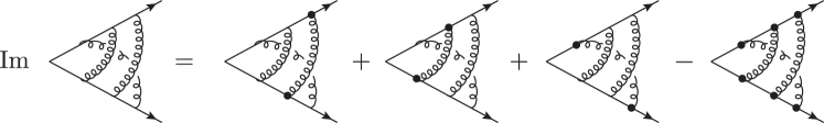
Figure 1: Schematic illustration of the formula (19) for the imaginary part of an eikonal diagram with no internal vertices. The black dots at the end points of a soft-gluon propagator indicate that the propagator has been cut; i.e., replaced by a delta function. Physically, the black dots represent the emission and absorption of a lightlike gauge boson. It is implied that the integrals over the attachment points of uncut soft propagators are principal-value integrals.

In order to extract the imaginary part of $F^{(L)}$ from the integral representation in Eq. (8) it will be useful to perform a change of variables which leaves each soft propagator dependent on a single variable. To this end, we adopt the change of variables introduced in Ref. Gardi:2011yz ,

$$\left(\begin{array}[]{c}t_{\ell_{j},m_{j}}\\ t_{r_{j},n_{j}}\end{array}\right)\hskip 0.56905pt=\hskip 0.56905pt\rho_{j}\left(\begin{array}[]{c}x_{j}\\ 1-x_{j}\end{array}\right)\hskip 8.53581pt\mathrm{where}\hskip 8.53581pt\left\{\begin{array}[]{l}0\leq\rho_{j}<\infty\\[2.27621pt] 0\leq x_{j}\leq 1\,.\end{array}\right.$$ (9)

For notational convenience, we define the nesting function in terms of the new variables as follows,

$$\Theta(\boldsymbol{\rho},\boldsymbol{x})\equiv\prod_{i=1}^{n}\prod_{k=0}^{N_{i}}\theta(t_{i,k+1}-t_{i,k})\bigg{|}_{\tiny\left(\begin{array}[]{c}t_{\ell_{j},m_{j}}\\ t_{r_{j},n_{j}}\end{array}\right)\hskip 1.99168pt=\hskip 1.99168pt\rho_{j}\left(\begin{array}[]{c}x_{j}\\ 1-x_{j}\end{array}\right)}\,,$$ (10)

and the soft propagators through

$$P_{ij}^{[\epsilon]}(x)\equiv\frac{v_{i}\cdot v_{j}}{\big{[}{-}\big{(}xv_{i}-(1-x)v_{j}\big{)}^{2}+i\eta\big{]}^{1-\epsilon}}\,.$$ (11)

The diagram then takes the form

$$F^{(L)}=\mu^{2L\epsilon}\prod_{j=1}^{L}\int_{0}^{\infty}\frac{{\rm d}\rho_{j}}{\rho_{j}^{1-2\epsilon}}\int_{0}^{1}{\rm d}x_{j}\hskip 1.13809ptP_{\ell_{j}r_{j}}^{[\epsilon]}(x_{j})\Theta(\boldsymbol{\rho},\boldsymbol{x})\,.$$ (12)

We observe that the dependence of the soft propagators on the radial coordinates $\rho_{j}$ has scaled out, and that each propagator now depends only on a single variable $x_{j}$.

Next, we extract the overall infrared divergence of the diagram by setting $\tau_{1}\equiv\rho_{1}$ and applying the following sequence of $L-1$ substitutions

$$\left(\begin{array}[]{c}\tau_{j}\\ \rho_{j+1}\end{array}\right)=\tau_{j+1}\left(\begin{array}[]{c}y_{j}\\ 1-y_{j}\end{array}\right)\hskip 11.38109pt\mathrm{with}\hskip 8.53581pt\left\{\begin{array}[]{l}0\leq\tau_{j}<\infty\\[0.28453pt] 0\leq y_{j}\leq 1\,,\end{array}\right.$$ (13)

where $j=1,\ldots,L-1$, the variables $\tau_{j}$ have the dimension of length, and the $y_{j}$ are dimensionless.

The $L$-loop eikonal diagram then becomes

$$F^{(L)}=\prod_{j=1}^{L}\int_{0}^{1}{\rm d}x_{j}\hskip 1.42262ptP_{\ell_{j}r_{j}}^{[\epsilon]}(x_{j})\hskip 1.13809pt\mathcal{I}(\boldsymbol{x})\,.$$ (14)

The infrared divergence of the diagram has been absorbed into the kernel

$$\mathcal{I}(\boldsymbol{x})=\Gamma(2L\epsilon)\left(\frac{\mu}{\Lambda}\right)^{2L\epsilon}\prod_{j=1}^{L-1}\int_{0}^{1}\frac{{\rm d}y_{j}\hskip 2.27621pty_{j}^{-1+2j\epsilon}}{(1-y_{j})^{1-2\epsilon}}\Theta\big{(}\{\boldsymbol{y},\boldsymbol{x}\}\big{)},$$ (15)

where the notation $\Theta\big{(}\{\boldsymbol{y},\boldsymbol{x}\}\big{)}$ refers to the result of applying the substitutions (13) to Eq. (10). Here we have regulated the infrared divergence through the damping factor $e^{-\Lambda\tau_{L}}$ with $\Lambda\ll 1$. In addition, Eq. (15) contains any potential ultraviolet subdivergences of the diagram.

Having written the $L$-loop eikonal diagram in the form (14), we now turn to the question of extracting its imaginary part. We will restrict our attention to the leading order in the dimensional regulator $\epsilon$ and drop the dependence of the soft propagators on $\epsilon$,

$$F^{(L)}=\prod_{j=1}^{L}\int_{0}^{1}{\rm d}x_{j}\hskip 1.42262ptP_{\ell_{j}r_{j}}^{[0]}(x_{j})\hskip 1.13809pt\mathcal{I}(\boldsymbol{x})\hskip 1.13809pt+\hskip 1.13809pt\mathcal{O}(\epsilon^{-d+1})\,,$$ (16)

with $d$ denoting the degree of divergence of the diagram, $F^{(L)}\sim\frac{1}{\epsilon^{d}}\times\mathrm{(finite)}$.

To compute the imaginary part of Eq. (16) we start by observing that Eq. (15) is manifestly real. The Feynman $i\eta$’s are thus the only source of imaginary parts of Eq. (16). We can therefore decompose each of the $x_{j}$-integration paths into a principal-value part and small semicircles around the propagator poles. As the integrand takes purely imaginary values in the regions close to the poles and is real-valued on the remaining domain of integration, the resulting $2^{L}$ terms (each involving $L$ integrations) will be either purely real or purely imaginary.

In order to collect the imaginary contributions, we define the cut propagator

$$\Delta_{ij}(x)\equiv-\pi\,v_{i}\cdot v_{j}\,\delta\big{(}(xv_{i}-(1-x)v_{j})^{2}\big{)}\,,$$ (17)

and the $p$-fold cutting operator

$$\operatorname{Cut}_{x_{i_{1}},\dotsc,x_{i_{p}}}F^{(L)} =\prod_{j=1\atop\!\!\!j\neq i_{1},\dotsc,i_{p}\!\!\!\!\!\!}^{n}\operatorname{PV}\int_{0}^{1}{\rm d}x_{j}\,P(x_{j})$$

$$\hskip 17.07164pt\times\prod_{k=1}^{p}\int_{0}^{1}{\rm d}x_{i_{k}}\,\Delta(x_{i_{k}})\hskip 0.85358pt\mathcal{I}(\boldsymbol{x})\,.$$ (18)

For notational brevity we omitted the indices on the (cut) propagators: $P(x_{j})\equiv P_{\ell_{j}r_{j}}^{[0]}(x_{j})$ and $\Delta(x_{j})\equiv\Delta_{\ell_{j}r_{j}}(x_{j})$.

The imaginary part of any $L$-loop eikonal diagram with no internal vertices is then, to the leading order in $\epsilon$,

$$\operatorname{\mathrm{Im}}F^{(L)}=\sum_{p=1\atop p\hskip 1.99168pt\text{odd}}^{L}\sum_{i_{1},\dotsc,i_{p}=1\atop i_{1}<\dotsm<i_{p}}^{L}i^{\,p-1}\operatorname{Cut}_{x_{i_{1}},\ldots,x_{i_{p}}}F^{(L)}\,.$$ (19)

The formula (19) is illustrated for a generic ladder diagram in Fig. 1. Note that Eq. (19) shows that the imaginary part of the integrated result for the diagram will have transcendentality weight one less than the real part.

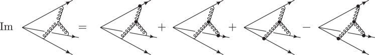
Figure 2: Schematic illustration of the formula (19) for the imaginary part of an eikonal diagram with an internal vertex.

We have verified the formula (19) for ladder-type diagrams with up to three loops, finding agreement with results in the literature . For example, for the diagram in Fig. 1, Eq. (19) yields the imaginary part ($\gamma\equiv\gamma_{12}$, $\chi\equiv e^{-\gamma}$)

$$\operatorname{\mathrm{Im}}F^{(3)} =\frac{\pi}{6\epsilon}\left(\frac{\mu}{\Lambda}\right)^{6\epsilon}\coth^{3}\gamma\hskip 0.85358pt\Big{[}H_{3,1}(\chi^{2})+H_{2,2}(\chi^{2})+H_{4}(\chi^{2})$$

$${-}\tfrac{1}{3}\log^{4}\chi+\log^{2}\chi\hskip 1.13809pt\big{(}H_{2}(\chi^{2})+3\zeta_{2}\big{)}-\log\chi\big{(}H_{3}(\chi^{2})-\zeta_{3}\big{)}$$

$$-\zeta_{2}H_{2}(\chi^{2})+\tfrac{1}{2}\zeta_{4}\Big{]}+\mathcal{O}(\epsilon^{0})\,.$$ (20)

The $H_{i,j}$ and $H_{i}$ denote harmonic polylogarithms according to the conventions of Ref. Remiddi:1999ew .

A natural question concerns the relation of the imaginary part of the eikonal diagram to the discontinuities in its various kinematic channels. Expressed in terms of the exponentials of the cusp angles, $\chi_{ij}\equiv e^{-\gamma_{ij}}$, rather than the cusp angles $\cosh\gamma_{ij}=|v_{i}\cdot v_{j}|$ themselves, the eikonal diagram has branch cuts located on the real line and satisfies Schwarz reflection, $F^{(L)}(\overline{\chi_{ij}})=\overline{F^{(L)}(\chi_{ij})}$. As a result, the discontinuities give rise to the imaginary part through the relation

$$2i\hskip 1.99168pt\mathrm{Im}\hskip 1.70717ptF^{(L)}(\boldsymbol{\chi})\hskip 1.99168pt=\hskip 1.99168pt\sum_{j=1}^{L}\theta(v_{\ell_{j}}\cdot v_{r_{j}})\hskip 0.56905pt\mathop{\mathrm{Disc}}_{\chi_{\ell_{j}r_{j}}}\hskip 0.85358ptF^{(L)}(\boldsymbol{\chi})\,.$$ (21)

The step functions account for the fact that the imaginary part has non-vanishing and vanishing contributions from channels with, respectively, timelike ($v_{\ell_{j}}\cdot v_{r_{j}}>0$) and spacelike ($v_{\ell_{j}}\cdot v_{r_{j}}<0$) kinematics, in agreement with the causality considerations of the previous section.

IV Cuts of eikonal diagrams with internal vertices

Eikonal diagrams with internal vertices have a more complicated structure than ladder-type diagrams. Nonetheless, we expect that our cutting prescription applies to such diagrams as well. As an explicit example, we consider the two-loop three-line diagram involving a three-gluon vertex, illustrated in Fig. 2. In order to apply our prescription, the overall infrared divergence of the diagram is extracted by integrating out the radial distance of the three-gluon vertex, leaving three remaining integrations over real projective space $u\in\mathds{R}\mathds{P}^{1,2}$. After some algebraic manipulations, the three-gluon vertex diagram has the following position-space representation, to the leading order in $\epsilon$ Mitov:2009sv ,

$$F_{3g}\propto\frac{1}{\epsilon}\int{\rm d}^{3}u\leavevmode\nobreak\ {\cal V}(\{v_{i}\},u)\hskip 1.13809pt\prod_{\ell=1}^{3}\int_{0}^{\infty}{\rm d}x_{\ell}\,P_{\ell}^{[0]}(\zeta_{\ell},x_{\ell})\,,$$ (22)

with the three-gluon vertex related differential operator ${\cal V}(\{v_{i}\},u)=\sum_{i,j,k=1}^{3}\varepsilon_{ijk}\,v_{i}\cdot v_{j}\,\zeta_{i}\,\zeta_{k}\,\frac{\partial}{\partial\zeta_{i}}$, in terms of the scalar products $\zeta_{i}=v_{i}\cdot u$. The position-space propagators are given by $P_{i}^{[\epsilon]}(\zeta_{i},x_{i})=(-u^{2}+2x_{i}\zeta_{i}-x_{i}^{2}+i\eta)^{-1+\epsilon}$. The imaginary part of this diagram is given by the formula (19) with the cut propagators,

$$\Delta_{i}(x)\equiv-\pi\,\delta\big{(}u^{2}-2x_{i}\zeta_{i}+x_{i}^{2}\big{)}\,.$$ (23)

The formula is illustrated in Fig. 2. We have checked the formula by performing the integral over the direction of the three-gluon vertex $u$ numerically. For small cusp angles, where the numerics proves to behave well, we find agreement with the analytic result in Ref. Ferroglia:2009ii . This in turn suggests the applicability of our cutting prescription to any eikonal diagram.

Acknowledgments

We thank S. Abreu, S. Caron-Huot, E. Gardi, J. Henn, P. Hoyer, L. Magnea, G. Sterman, I. Stewart, W. Vleeshouwers, A. Waelkens, C. White and especially G. Korchemsky for useful discussions. KJL is grateful for the hospitality of the Institute for Advanced Study in Princeton and the Institut de Physique Théorique, CEA Saclay, where part of this work was carried out. The research leading to these results has received funding from the European Union Seventh Framework Programme (FP7/2007-2013) under grant agreement no. 627521. This work was supported by the Foundation for Fundamental Research of Matter (FOM), program 104 “Theoretical Particle Physics in the Era of the LHC” and by the Research Executive Agency (REA) of the European Union under the Grant Agreement number PITN-GA-2010-264564 (LHCPhenoNet).

References

- (1) D. Yennie, S. C. Frautschi, and H. Suura, Annals Phys. 13, 379 (1961).
- (2) J. Gatheral, Phys.Lett. B133, 90 (1983).
- (3) J. Frenkel and J. Taylor, Nucl.Phys. B246, 231 (1984).
- (4) E. Gardi, E. Laenen, G. Stavenga, and C. D. White, JHEP 1011, 155 (2010), 1008.0098.
- (5) A. Mitov, G. Sterman, and I. Sung, Phys.Rev. D82, 096010 (2010), 1008.0099.
- (6) E. Gardi, J. M. Smillie, and C. D. White, JHEP 1306, 088 (2013), 1304.7040.
- (7) G. Korchemsky and A. Radyushkin, Phys.Lett. B171, 459 (1986).
- (8) G. Korchemsky and A. Radyushkin, Nucl. Phys. B283, 342 (1987).
- (9) S. M. Aybat, L. J. Dixon, and G. F. Sterman, Phys.Rev.Lett. 97, 072001 (2006), hep-ph/0606254.
- (10) S. M. Aybat, L. J. Dixon, and G. F. Sterman, Phys.Rev. D74, 074004 (2006), hep-ph/0607309.
- (11) T. Becher and M. Neubert, Phys.Rev. D79, 125004 (2009), 0904.1021.
- (12) A. Ferroglia, M. Neubert, B. D. Pecjak, and L. L. Yang, Phys.Rev.Lett. 103, 201601 (2009), 0907.4791.
- (13) A. Ferroglia, M. Neubert, B. D. Pecjak, and L. L. Yang, JHEP 0911, 062 (2009), 0908.3676.
- (14) A. Mitov, G. F. Sterman, and I. Sung, Phys.Rev. D82, 034020 (2010), 1005.4646.
- (15) J. M. Henn and T. Huber, JHEP 1309, 147 (2013), 1304.6418.
- (16) E. Gardi, JHEP 1404, 044 (2014), 1310.5268.
- (17) G. Falcioni, E. Gardi, M. Harley, L. Magnea, and C. D. White, JHEP 1410, 10 (2014), 1407.3477.
- (18) N. Kidonakis, Phys.Rev.Lett. 102, 232003 (2009), 0903.2561.
- (19) A. Grozin, J. M. Henn, G. P. Korchemsky, and P. Marquard, (2014), 1409.0023.
- (20) J. R. Forshaw, A. Kyrieleis, and M. Seymour, JHEP 0608, 059 (2006), hep-ph/0604094.
- (21) J. Forshaw, A. Kyrieleis, and M. Seymour, JHEP 0809, 128 (2008), 0808.1269.
- (22) G. Korchemsky and G. Marchesini, Nucl.Phys. B406, 225 (1993), hep-ph/9210281.
- (23) E. Gardi, JHEP 0502, 053 (2005), hep-ph/0501257.
- (24) S. Catani, D. de Florian, and G. Rodrigo, JHEP 1207, 026 (2012), 1112.4405.
- (25) J. R. Forshaw, M. H. Seymour, and A. Siodmok, JHEP 1211, 066 (2012), 1206.6363.
- (26) Z. Bern, L. J. Dixon, D. C. Dunbar, and D. A. Kosower, Nucl.Phys. B425, 217 (1994), hep-ph/9403226.
- (27) Z. Bern, L. J. Dixon, D. C. Dunbar, and D. A. Kosower, Nucl.Phys. B435, 59 (1995), hep-ph/9409265.
- (28) Z. Bern, L. J. Dixon, and D. A. Kosower, Ann.Rev.Nucl.Part.Sci. 46, 109 (1996), hep-ph/9602280.
- (29) R. Britto, F. Cachazo, and B. Feng, Nucl.Phys. B725, 275 (2005), hep-th/0412103.
- (30) R. Britto, E. Buchbinder, F. Cachazo, and B. Feng, Phys.Rev. D72, 065012 (2005), hep-ph/0503132.
- (31) D. Forde, Phys.Rev. D75, 125019 (2007), 0704.1835.
- (32) P. Mastrolia, Phys.Lett. B678, 246 (2009), 0905.2909.
- (33) D. A. Kosower and K. J. Larsen, Phys.Rev. D85, 045017 (2012), 1108.1180.
- (34) S. Caron-Huot and K. J. Larsen, JHEP 1210, 026 (2012), 1205.0801.
- (35) Y.-T. Chien, M. D. Schwartz, D. Simmons-Duffin, and I. W. Stewart, Phys.Rev. D85, 045010 (2012), 1109.6010.
- (36) J. C. Collins, D. E. Soper, and G. F. Sterman, Phys.Lett. B134, 263 (1984).
- (37) E. Gardi, J. M. Smillie, and C. D. White, JHEP 1109, 114 (2011), 1108.1357.
- (38) E. Remiddi and J. Vermaseren, Int.J.Mod.Phys. A15, 725 (2000), hep-ph/9905237.
- (39) A. Mitov, G. F. Sterman, and I. Sung, Phys.Rev. D79, 094015 (2009), 0903.3241.