Variational Reformulation of Bayesian Inverse Problems

Abstract

The classical approach to inverse problems is based on the optimization of a misfit function. Despite its computational appeal, such an approach suffers from many shortcomings, e.g., non-uniqueness of solutions, modeling prior knowledge, etc. The Bayesian formalism to inverse problems avoids most of the difficulties encountered by the optimization approach, albeit at an increased computational cost. In this work, we use information theoretic arguments to cast the Bayesian inference problem in terms of an optimization problem. The resulting scheme combines the theoretical soundness of fully Bayesian inference with the computational efficiency of a simple optimization.

1 Introduction

As we are approaching the era of exascale computing, we encounter more and more complex physical models. These complex models have many unknown parameters that need to be inferred from experimental measurements. That is, inverse problems are becoming an integral part of every scientific discipline that attempts to combine computational models with data. These include climate modeling [4], numerical weather prediction [18, 25], subsurface hydrology and geology [15], and many more.

It can be argued that the “right” way to pose an inverse problem is to follow the Bayesian formalism [28, 17]. It is the “right” way because it deals with three well-known difficulties of inverse problems: non-uniqueness issues, modeling prior knowledge, and estimating experimental noise. The Bayesian solution of an inverse problem is summarized neatly by the posterior probability density of the quantity of interest. In turn, the posterior can only be explored numerically by Monte Carlo (MC) methods, the most successful of which is Markov Chain Monte Carlo (MCMC) [24, 14]. Because of the need to repeatedly evaluate the underlying physical model, MCMC is computationally impractical for all but the simplest cases. Therefore, we need methods that approximate the posterior in a computationally efficient manner.

One way to come up with a computationally attractive approximation is to replace the physical model with a cheap-to-evaluate surrogate [20, 22]. In this way, MCMC becomes feasible again. However, there is no free lunch: firstly, things become complicated when the surrogate is inaccurate, and, secondly, constructing accurate surrogates is exponentially hard as the number of parameters increase [3]. Because of these difficulties, in this work, we attempt to develop a surrogate-free methodology.

Perhaps the simplest idea is to approximate the posterior with a delta function centered about its maximum. The maximum of the posterior is known as the maximum a posteriori (MAP) estimate of the parameters. The MAP approach is justified if the posterior is sharply picked around a unique maximum. It requires the solution of an optimization problem. The objective function of this optimization has two parts: a misfit and a regularization part that arise from the likelihood and the prior, respectively. The MAP estimate is commonly used in numerical weather prediction problems [25] as well as in seismic inversion [8].

The Laplace approximation represents the posterior by a Gaussian density with a mean given by the MAP and a covariance matrix given by the negative inverse Hessian of the logarithm of the posterior. The Laplace approximation is justified when the posterior has a unique maximum and is shaped, more or less, like a Gaussian around it. As before, the identification of the MAP requires the solution of an optimization problem. The required Hessian information may be estimated numerically either by automatic differentiation methods [12] or by developing the adjoint equations of the underlying physical model [26].

Variational inference (VI) [10, 7] is a class of techniques in Bayesian statistics targeted toward the construction of approximate posteriors. One proceeds by posing a variational problem whose solution over a family of probability densities approximates the posterior. VI techniques have been proved quite effective for a wide class of inference problems. However, in their archetypal form, they are not directly applicable to inverse problems. This is due to the, typically, non-analytic nature of the underlying physical models. Fortunately, the recent developments in non-parametric VI by [11] can come to rescue. This is the approach we follow in this work. In non-parametric VI, the family of probability densities that serve as candidate posteriors is the family of mixtures of Gaussians with a fixed number of components [23]. Since a mixture of Gaussians with an adequate number of components can represent any probability density, this approximating family is sufficiently large. The approximate posterior is constructed by minimizing the information loss between the true posterior and the approximate one over the candidate family. This is achieved by solving a series of optimization problems [7].

The outline of the paper is as follows. We start section 2 with a generic discussion of the Bayesian formulation of inverse problems. In section 2.1 we present the core ideas of VI and in section 2.2 we show how one can develop approximation schemes. We validate the proposed methodology numerically by solving two inverse problems: the estimation of the kinetic parameters of a catalysis system (section 3.1) and the identification of the source of contamination based on scarce concentration measurements (section 3.2). Finally, in 0.A we provide all the technical details that are required for the implementation of the proposed methodology.

2 Methodology

A forward model associated with a physical phenomenon can be thought of as a function $\mathbf{f}:\mathbb{R}^{d_{\xi}}\rightarrow\mathbb{R}^{d_{y}}$, that connects some unknown parameters $\boldsymbol{\xi}\in\mathbb{R}^{d_{\xi}}$ to some observed quantities $\mathbf{y}\in\mathbb{R}^{d_{y}}$. This connection is defined indirectly via a likelihood function:

$$p(\mathbf{y}|\boldsymbol{\xi},\boldsymbol{\theta})=p(\mathbf{y}|\mathbf{f}(\boldsymbol{\xi}),\boldsymbol{\theta}),$$ (1)

where $\boldsymbol{\theta}\in\mathbb{R}^{d_{\theta}}$ denotes the parameters that control the measurement noise and/or the model discrepancy. Notice how in Eq. (1) the observations, $\mathbf{y}$, are explicitly connected to the parameters, $\boldsymbol{\xi}$, through the model, $\mathbf{f}(\boldsymbol{\xi})$. A typical example of a likelihood function is the isotropic Gaussian likelihood:

$$p(\mathbf{y}|\boldsymbol{\xi},\theta)=\mathcal{N}\left(\mathbf{y}|\mathbf{f}(\boldsymbol{\xi}),e^{2\theta}\mathbf{I}\right),$$ (2)

where $\theta$ is a real number, and $\mathbf{I}$ is the unit matrix with the same dimensions as $\mathbf{y}$. The exponential of the parameter,

$$\sigma=e^{\theta},$$ (3)

can be thought of as the standard deviation of the measurement noise. The usual parameterization of the isotropic Gaussian likelihood uses $\sigma$ instead of $\theta$. We do not follow the usual approach because in our numerical examples, it is preferable to work with real rather than positive numbers.

Both $\boldsymbol{\xi}$ and $\boldsymbol{\theta}$ are characterized by prior probability densities, $p(\boldsymbol{\xi})$ and $p(\boldsymbol{\theta})$, respectively. These describe our state of knowledge, prior to observing $\mathbf{y}$. As soon as $\mathbf{y}$ is observed, our updated state of knowledge is captured by the posterior distribution:

$$p(\boldsymbol{\xi},\boldsymbol{\theta}|\mathbf{y})=\frac{p(\mathbf{y}|\boldsymbol{\xi},\boldsymbol{\theta})p(\boldsymbol{\xi})p(\boldsymbol{\theta})}{p(\mathbf{y})},$$ (4)

where the normalization constant $p(\mathbf{y})$,

$$p(\mathbf{y})=\int p(\mathbf{y}|\boldsymbol{\xi},\boldsymbol{\theta})p(\boldsymbol{\xi})p(\boldsymbol{\theta})d\boldsymbol{\xi}d\boldsymbol{\theta},$$ (5)

is known as the evidence. Eq. (4) is the Bayesian solution to the inverse problem. Notice that it is a probability density over the joint space of $\boldsymbol{\xi}$ and $\boldsymbol{\theta}$. This is to be contrasted with the classical approaches to inverse problems whose solutions result in point estimates of the unknown variables. The mass of this probability density corresponds to our inability to fully resolve the values of $\boldsymbol{\xi}$ and $\boldsymbol{\theta}$ due to insufficient experimental information.

Notice that by writing $\boldsymbol{\omega}=(\boldsymbol{\xi},\boldsymbol{\theta})\in\mathbb{R}^{d}$,$d=d_{\xi}+d_{\omega}$, $p(\boldsymbol{\omega})=p(\boldsymbol{\xi})p(\boldsymbol{\theta})$, and $p(\mathbf{y}|\boldsymbol{\omega})=p(\mathbf{y}|\boldsymbol{\xi},\boldsymbol{\theta})$, we may simplify the notation of Eq. (4) to

$$p(\boldsymbol{\omega}|\mathbf{y})=\frac{p(\mathbf{y}|\boldsymbol{\omega})p(\boldsymbol{\omega})}{p(\mathbf{y})}.$$ (6)

This is the notation we follow through out this work. The goal of the rest of the paper is to construct an algorithmic framework for the efficient approximation of the posterior of Eq. (6).

2.1 Variational inference

Consider a family $\mathcal{Q}$ of probability densities over $\boldsymbol{\omega}$. Our objective is to choose a $q(\boldsymbol{\omega})\in\mathcal{Q}$ that is as “close” as possible to the posterior $p(\boldsymbol{\omega}|\mathbf{y})$ of Eq. (6). This “closeness” is measured by the Kullback-Leibler (KL) divergence [21],

$$\mbox{KL}\left[q(\boldsymbol{\omega})\parallel p(\boldsymbol{\omega}|\mathbf{y})\right]=\mathbb{E}_{q}\left[\log\frac{q(\boldsymbol{\omega})}{p(\boldsymbol{\omega}|\mathbf{y})}\right],$$ (7)

where $\mathbb{E}_{q}\left[\cdot\right]$ denotes the expectation with respect to $q(\boldsymbol{\omega})$. Intuitively, the KL divergence can be thought of as the information loss we experience when we approximate the posterior $p(\boldsymbol{\omega}|\mathbf{y})$ with the probability density $q(\boldsymbol{\omega})$. It is easy to show that

$$\mbox{KL}\left[q(\boldsymbol{\omega})\parallel p(\boldsymbol{\omega}|\mathbf{y})\right]\geq 0,$$ (8)

and that the equality holds if and only if $q(\boldsymbol{\omega})=p(\boldsymbol{\omega}|\mathbf{y})$. Therefore, if the posterior is in $\mathcal{Q}$, then minimizing Eq. (7) over $q(\omega)\in\mathcal{Q}$ will give an exact answer. For an arbitrary choice of $\mathcal{Q}$, we postulate that minimizing Eq. (7) yields a good approximation to the posterior.

Unfortunately, calculation of Eq. (7) requires knowledge of the posterior. This means that Eq. (7) cannot be used directly in an optimization scheme. In order to proceed, we need an objective function that does not depend explicitly on the posterior. To this end, notice that the evidence may be expressed as:

$$\log p(\mathbf{y})=\mathcal{F}\left[q\right]+\mbox{KL}\left[q(\boldsymbol{\omega})\parallel p(\boldsymbol{\omega}|\mathbf{y})\right],$$ (9)

where

$$\mathcal{F}\left[q\right]=\mathbb{E}_{q}\left[\log\frac{p(\mathbf{y},\boldsymbol{\omega})}{q(\boldsymbol{\omega})}\right]=\mathcal{H}\left[q\right]+\mathbb{E}_{q}\left[\log p(\mathbf{y},\boldsymbol{\omega})\right],$$ (10)

with

$$p(\mathbf{y},\boldsymbol{\omega})=p(\mathbf{y}|\boldsymbol{\omega})p(\boldsymbol{\omega})$$ (11)

being the joint probability density of $\mathbf{y}$ and $\boldsymbol{\omega}$, and

$$\mathcal{H}[q]=-\mathbb{E}_{q}\left[\log q(\boldsymbol{\omega})\right]$$ (12)

being the entropy of $q(\boldsymbol{\omega})$. Since the KL divergence is non-negative (Eq. (8)), we have from Eq. (9) that

$$\mathcal{F}[q]\leq\log p(\mathbf{y}).$$ (13)

The functional $\mathcal{F}[q]$ is generally known as the evidence lower bound (ELBO).

We see, that maximizing Eq. (10) is equivalent to minimizing Eq. (7). In addition, Eq. (10) does not depend on the posterior in an explicit manner. This brings us to the variational principle used through out this work: The “best” approximation to the posterior of Eq. (6) over the family of probability densities $\mathcal{Q}$ is the solution to the following optimization problem:

$$q^{*}(\boldsymbol{\omega})=\arg\max_{q}\mathcal{F}[q].$$ (14)

2.2 Developing approximation schemes

The main difficulty involved in the solution Eq. (14) is the evaluation of expectations over $q(\boldsymbol{\omega})$. In principle, one can approximate these expectations via a Monte Carlo procedure and, then, use a variant of the Robbins-Monro algorithm [27]. Such an approach yields a stochastic optimization scheme in the spirit of [5], and [2]. Whether or not such a scheme is more efficient than MCMC sampling of the posterior is beyond the scope of this work. Here, we follow the approach outlined by [11]. In particular, we will derive analytical approximations of $\mathcal{F}[q]$ for the special case in which $\mathcal{Q}$ is the family of Gaussian mixtures.

The family of Gaussian mixtures with $L$ components is the family $\mathcal{Q}_{L}$ of probability densities of the form:

$$q(\boldsymbol{\omega})=\sum_{i=1}^{L}w_{i}\mathcal{N}(\boldsymbol{\omega}|\boldsymbol{\mu}_{i},\boldsymbol{\Sigma}_{i})$$ (15)

where $w_{i}$, $\boldsymbol{\mu}_{i}$ and $\boldsymbol{\Sigma}_{i}$ are the responsibility, mean, and covariance matrix, respectively, of the $i$-th component of the mixture. The responsibilities $w_{i}$ are non-negative and they sum to one while the covariance matrices $\boldsymbol{\Sigma}_{i}$ are positive definite. When we work with $\mathcal{Q}_{L}$, the generic variational problem of Eq. (6) is equivalent to optimization with respect to all the $w_{i},\boldsymbol{\mu}_{i}$ and $\boldsymbol{\Sigma}_{i}$. In what follows, we replace the ELBO, $\mathcal{F}[q]$ of Eq. (10), with a series of analytic approximations that exploit the properties of $\mathcal{Q}_{L}$, and, finally, we derive a three-step optimization scheme that yields a local maximum of the approximate ELBO.

We start with an approximation to the entropy $\mathcal{H}[q]$ (see Eq. (12)) of a Gaussian mixture Eq. (15). There are basically two kinds of approximations that may be derived: 1) using Jensen’s inequality yields a lower bound to $\mathcal{H}[q]$ built out of convolutions of Gaussians (see [11] and [16]), and 2) employing a Taylor expansion of $\log q(\boldsymbol{\omega})$ about each $\boldsymbol{\mu}_{i}$ and evaluating the expectation over $\mathcal{N}(\boldsymbol{\omega}|\boldsymbol{\mu}_{i},\boldsymbol{\Sigma}_{i})$ (see [16]). We have experimented with both approximations to the entropy without observing any significant differences in the numerical results. Therefore, we opt for the former one since it has a very simple analytical form. An application of Jensen’s inequality followed by well-known results about the convolution of two Gaussians yields

$$\mathcal{H}[q]\geq\mathcal{H}_{0}[q],$$ (16)

where

$$\mathcal{H}_{0}[q]=-\sum_{i=1}^{L}w_{i}\ln q_{i},$$ (17)

with

$$q_{i}=\sum_{j=1}^{L}w_{j}\mathcal{N}(\boldsymbol{\mu}_{i}|\boldsymbol{\mu}_{j},\boldsymbol{\Sigma}_{i}+\boldsymbol{\Sigma}_{j}).$$ (18)

The idea is to simply replace $\mathcal{H}[q]$ in Eq. (10) with $\mathcal{H}_{0}[q]$ of Eq. (17). This results in a lower bound to the ELBO $\mathcal{F}[q]$.

Now, we turn our attention to the second term of Eq. (10). For convenience, let us write it as:

$$\mathcal{L}[q]=\mathbb{E}_{q}\left[\log p(\mathbf{y},\boldsymbol{\omega})\right].$$ (19)

Notice that $\mathcal{L}[q]$ may be expanded as:

$$\mathcal{L}[q]=\sum_{i=1}^{L}w_{i}\mathbb{E}_{\mathcal{N}(\boldsymbol{\omega}|\boldsymbol{\mu}_{i},\boldsymbol{\Sigma}_{i})}\left[\log p(\mathbf{y},\boldsymbol{\omega})\right],$$ (20)

and that each expectation term can be approximated by taking the Taylor expansion of $\log p(\mathbf{y},\boldsymbol{\omega})$ about $\boldsymbol{\omega}=\boldsymbol{\mu}_{i}$:

$$\begin{array}[]{ccc}\log p(\mathbf{y},\boldsymbol{\omega})&\approx&\log p(\mathbf{y},\boldsymbol{\omega}=\boldsymbol{\mu}_{i})+\nabla_{\boldsymbol{\omega}}\log p(\mathbf{y},\boldsymbol{\omega}=\boldsymbol{\mu}_{i})\left(\boldsymbol{\omega}-\boldsymbol{\mu}_{i}\right)\\ &&+\frac{1}{2}(\boldsymbol{\omega}-\boldsymbol{\mu}_{i})^{T}\nabla^{2}_{\boldsymbol{\omega}}\log p(\mathbf{y},\boldsymbol{\omega}=\boldsymbol{\mu}_{i})(\boldsymbol{\omega}-\boldsymbol{\mu}_{i}),\end{array}$$ (21)

where $\nabla_{\boldsymbol{\omega}}$ and $\nabla_{\boldsymbol{\omega}}^{2}$ stand for the Jacobian and the Hessian with respect to $\boldsymbol{\omega}$, respectively. Combining Eq. (20) with Eq. (21), we get the zero and second order Taylor approximation to $\mathcal{L}[q]$ of Eq. (19),

$$\mathcal{L}_{0}[q]=\sum_{i=1}^{L}w_{i}\log p(\mathbf{y},\boldsymbol{\omega}=\boldsymbol{\mu}_{i}),$$ (22)

and

$$\mathcal{L}_{2}[q]=\mathcal{L}_{0}[q]+\frac{1}{2}\sum_{i=1}^{L}w_{i}\mbox{Tr}\left[\boldsymbol{\Sigma}_{i}\nabla_{\boldsymbol{\omega}}^{2}\log p(\mathbf{y},\boldsymbol{\omega}=\boldsymbol{\mu}_{i})\right],$$ (23)

respectively.

Combining Eq. (17) with Eq. (22) or Eq. (23) we get an approximation to Eq. (10). In particular, we define:

$$\mathcal{F}_{a}[q]=\mathcal{H}_{0}[q]+\mathcal{L}_{a}[q],$$ (24)

where $a=1$, or $2$, selects the approximation to Eq. (19). From this point on, our goal is to derive an algorithm that converges to a local maximum of $\mathcal{F}_{2}[q]$.

Notice that $\mathcal{F}_{2}[q]$ requires the Hessian of $\log p(\mathbf{y},\boldsymbol{\omega})$ at $\boldsymbol{\omega}=\boldsymbol{\mu}_{i}$. Therefore, optimizing it with respect to $\boldsymbol{\mu}_{i}$ would require third derivatives of $\log p(\mathbf{y},\boldsymbol{\omega})$. This, in turn, implies the availability of third derivatives of the forward model $\mathbf{f}(\boldsymbol{\xi})$. Getting third derivatives of the forward model is impractical in almost all cases. In contrast, optimization of $\mathcal{F}_{0}[q]$ with respect to $\boldsymbol{\mu}_{i}$ requires only first derivatives of $\log p(\mathbf{y},\boldsymbol{\omega})$, i.e., only first derivatives of the forward model $\mathbf{f}(\boldsymbol{\xi})$. In many inverse problems of interest, derivatives can be obtained at a minimum cost by making use of adjoint techniques (e.g., [9]). Therefore, optimization of $\mathcal{F}_{00}[q]$ with respect to $\boldsymbol{\mu}_{i}$ is computationally feasible.

The situation for $\boldsymbol{\Sigma}_{i}$ is quite different. Firstly, notice that $\mathcal{H}_{0}[q]$ increases logarithmically without bounds as a function of $|\boldsymbol{\Sigma}_{i}|$ and that the $\mathcal{L}_{0}[q]$ does not depend on $\boldsymbol{\Sigma}_{i}$ at all. We see that the lowest approximation that carries information about $\boldsymbol{\Sigma}_{i}$ is $\mathcal{F}_{2}[q]$. Looking at Eq. (23) we observe that this information is conveyed via the Hessian of $\log p(\mathbf{y},\boldsymbol{\omega})$. This, in turn, requires the Hessian of the forward model $\mathbf{f}(\boldsymbol{\xi})$. The latter is a non-trivial task which is, however, feasible. In addition, notice that if $\boldsymbol{\Sigma}_{i}$ is restricted to be diagonal, then only the diagonal part of the Hessian of $\log p(\mathbf{y},\boldsymbol{\omega})$ is required, thus, significantly reducing the memory requirements. The computation of $F_{2}[q]$ as well as of its gradients with respect to $w_{i},\boldsymbol{\mu}_{i}$, and $\boldsymbol{\Sigma}_{i}$ is discussed in 0.A.

Taking the above into account, we propose an optimization scheme that alternates between optimizing $\{\boldsymbol{\mu}_{i}\}_{i=1}^{L}$, $\{\boldsymbol{\Sigma}_{i}\}_{i=1}^{L}$, and $\{w_{i}\}_{i=1}^{L}$. The algorithm is summarized in Algorithm 1. However, in order to avoid the use of third derivatives of the forward model we follow [11] in using $\mathcal{F}_{0}[q]$ as the objective function when optimizing for $\{\boldsymbol{\mu}_{i}\}$. Furthermore, we restrict our attention to diagonal covariance matrices,

$$\boldsymbol{\Sigma}_{i}=\mbox{diag}\left(\sigma_{i1}^{2},\dots,\sigma_{id}^{2}\right),$$ (25)

since we do not want to deal with the issue of enforcing positive definiteness of the $\boldsymbol{\Sigma}_{i}$’s during their optimization. We use the L-BFGS-B algorithm of [6], which can perform bound constrained optimization. The bounds we use are problem-specific and are discussed in section 3. In all numerical examples, we use the same convergence tolerance $\epsilon=10^{-2}$.

Input : Data $\mathbf{y}$, number of components $L$.

Initialize : $w_{i}=1/N,\boldsymbol{\Sigma}_{i}=I$, and $\boldsymbol{\mu}_{i}$ randomly, for $i=1,\dots,L$.

repeat

       for $i=1$ to $L$ do

             $\{\boldsymbol{\mu}_{i}\}\leftarrow\arg\max_{\{\boldsymbol{\mu}_{i}\}}\mathcal{F}_{0}[q]$

             $\{w_{i}\}\leftarrow\arg\max_{\{w_{i}\}}\mathcal{F}_{2}[q]$

             $\{\boldsymbol{\Sigma}_{i}\}\leftarrow\arg\max_{\left\{\boldsymbol{\Sigma}_{i}=\mbox{diag}\left(\sigma_{i1}^{2},\dots,\sigma_{id}^{2}\right)\right\}}\mathcal{F}_{2}[q]$

       end for

      

until  change in $\mathcal{F}_{2}[q]$ is less than a tolerance $\epsilon$

Algorithm 1 Variational Inference

3 Examples

In this section we present two numerical examples: 1) The problem of estimating rate constants in a catalysis system (section 3.1), and 2) the problem of identifying the source of contamination in a two dimensional domain (section 3.2). In both examples, we compare the approximate posterior to a MCMC [14] estimate. We used the Metropolis-Adjusted-Langevin-Algorithm (MALA) [1], since it can use the derivatives of the forward models to accelerate convergence. In all examples, the step size of the MALA proposal was $dt=0.1$, the first $1,000$ steps were burned, and we observed the chain every $100$ steps for a total of $100,000$ steps. We implented our methodology is Python. The code is freely available at https://github.com/ebilionis/variational-reformulation-of-inverse-problems.

3.1 Reaction kinetic model

We consider the problem of estimating kinetic parameters of multi-step chemical reactions that involve various intermediate or final products. In particular, we study the dynamical system that describes the catalytic conversion of nitrate ($\mbox{NO}_{3}^{-}$) to nitrogen ($\mbox{N}_{2}$) and other by-products by electrochemical means. The mechanism that is followed is complex and not well understood. In this work, we use the simplified model proposed by [19], which includes the production of nitrogen ($\mbox{N}_{2}$), ammonia ($\mbox{NH}_{3}$), and nitrous oxide ($\mbox{N}_{2}\mbox{O}$) as final products, as well as that of nitrite ($\mbox{NO}_{2}^{-}$) and an unknown species X as reaction intermediates (see figure 1).

Figure 1: Reaction kinetic model: Simplified reaction scheme for the reduction of nitr4ate.

The dynamical system associated with the reaction depicted in figure 1 is:

$$\begin{array}[]{cc}\frac{d[\mbox{NO}_{3}^{-}]}{dt}&=-k_{1}[\mbox{NO}_{3}^{-}],\\ \frac{d[\mbox{NO}_{2}^{-}]}{dt}&=k_{1}[\mbox{NO}_{3}^{-}]-(k_{2}+k_{4}+k_{5})[\mbox{NO}_{2}^{-}],\\ \frac{d[\mbox{X}]}{dt}&=k_{2}[\mbox{NO}_{2}^{-}]-k_{3}[X],\\ \frac{d[\mbox{N}_{2}]}{dt}&=k_{3}[\mbox{X}],\\ \frac{d[\mbox{NH}_{3}]}{dt}&=k_{4}[\mbox{NO}_{2}^{-}],\\ \frac{d[\mbox{N}_{2}O]}{dt}&=k_{5}[\mbox{NO}_{2}^{-}],\end{array}$$ (26)

where $[\cdot]$ denotes the concentration of a quantity, and $k_{i}>0$, $i=1,...5$ are the kinetic rate constants. Our goal is to estimate the kinetic rate constants based on the experimental measurements obtained by [19]. For completeness, these measurements are reproduced in table 1. The initial conditions for Eq. (26) are given by the $t=0$ row of the table 1.

$t$ (min)	$[\mbox{NO}_{3}^{-}]$	$[\mbox{NO}_{2}^{-}]$	$[\mbox{X}]$	$[\mbox{N}_{2}]$	$[\mbox{NH}_{3}]$	$[\mbox{N}_{2}\mbox{O}]$
0	500.00	0.00	-	0.00	0.00	0.00
30	250.95	107.32	-	18.51	3.33	4.98
60	123.66	132.33	-	74.85	7.34	20.14
90	84.47	98.81	-	166.19	13.14	42.10
120	30.24	38.74	-	249.78	19.54	55.98
150	27.94	10.42	-	292.32	24.07	60.65
180	13.54	6.11	-	309.50	27.26	62.54

Table 1: Reaction kinetic model: The table contains the experimental data used in the calibration process. The rows correspond to the time of each measurement and the columns to the concentrations measured in $\mbox{mmol}\cdot\mbox{L}^{-1}$. The “-” symbols corresponds to lack of observations. See [19] for more details on the experiment. The $t=0$ row provides the initial condition to Eq. (26). The observed data vector $\mathbf{y}\in\mathbb{R}^{30}$ is built by concatenating the scaled version of the rows $t=30$ to $t=180$ while skipping the row corresponding to X.

In order to avoid numerical instabilities, we work with a dimensionless version of Eq. (26). In particular, we define the scaled time:

$$\tau=\frac{t}{180\;\mbox{min}},$$ (27)

the scaled concentrations:

$$u_{i}=\frac{[\mbox{Y}]}{500\;\mbox{mmol}\cdot\mbox{L}^{-1}},$$ (28)

for $i=1,2,3,4,5,6,7$, and $\mbox{Y}=\mbox{NO}_{3}^{-},\mbox{NO}_{2}^{-},\mbox{X},\mbox{N}_{2},\mbox{NH}_{3},\mbox{N}_{2}\mbox{O}$, respectively, and the scaled kinetic rate constants:

$$\kappa_{i}=k_{i}\cdot 180\;\mbox{min},$$ (29)

for $i=1,\dots,5$. The dimensionless dynamical system associated with Eq. (26) is:

$$\begin{array}[]{cc}\dot{u}_{1}&=-\kappa_{1}u_{1},\\ \dot{u}_{2}&=\kappa_{1}u_{1}-(\kappa_{2}+\kappa_{4}+\kappa_{5})u_{2},\\ \dot{u}_{3}&=\kappa_{2}u_{2}-\kappa_{3}u_{3},\\ \dot{u}_{4}&=\kappa_{3}u_{3},\\ \dot{u}_{5}&=\kappa_{4}u_{2},\\ \dot{u}_{6}&=\kappa_{5}u_{2},\end{array}$$ (30)

where $\dot{u}$ denotes the differentiation of $u$ with respect to the scaled time $\tau$. The initial conditions for Eq. (30) are given by the scaled version of the $t=0$ row of table 1. We arrange the scaled version of the experimental data of table 1 in a vector form, $\mathbf{y}\in\mathbb{R}^{d_{y}}$ with $d_{y}=30$, by concatenating rows $t=30,\dots,180$ of table 1 while skipping the third column.

Table 2: Reaction kinetic model: The logarithm of the scaled kinetic rate constants, $\xi_{i}$ (see Eq. (31), and the logarithm of the likelihood noise, $\theta$ (see Eq. (2)) as estimated by the variational approach with $L=1$ and MCMC (MALA). The estimates correspond to the mean and the uncertainties to two times the standard deviation of each method.

Variable	VAR ($L=1$)	MCMC (MALA)
$\xi_{1}$	$1.359\pm 0.055$	$1.356\pm 0.072$
$\xi_{2}$	$1.657\pm 0.086$	$1.664\pm 0.142$
$\xi_{3}$	$1.347\pm 0.118$	$1.349\pm 0.215$
$\xi_{4}$	$-0.162\pm 0.167$	$-0.159\pm 0.230$
$\xi_{5}$	$-1.009\pm 0.368$	$-1.071\pm 0.513$
$\theta$	$-3.840\pm 0.204$	$-3.757\pm 0.251$

Since the kinetic rate constants, $\kappa_{i}$, of the scaled dynamical system of Eq. (30) are non-negative, it is problematic to attempt to approximate the posteriors associated with them with mixtures of Gaussians. For this reason, we work with the logarithms of the $\kappa_{i}$’s,

$$\xi_{i}=\log\kappa_{i},$$ (31)

for $i=1,\dots,5$. We collectively denote those variables by $\boldsymbol{\xi}=(\xi_{1},\dots,\xi_{5})$. The prior probability density we assign to $\boldsymbol{\xi}$ is:

$$p(\boldsymbol{\xi})=\prod_{i=1}^{5}p(\xi_{i}),$$ (32)

with

$$p(\xi_{i})=\mathcal{N}(\xi_{i}|0,1),$$ (33)

for $i=1,\dots,5$.

Rate constant	Katsounaros (2012)	VAR Median	VAR 95% Interval
$k_{1}$	$0.0216\pm 0.0014$	0.0216	(0.0205, 0.0229)
$k_{2}$	$0.0292\pm 0.0036$	0.0291	(0.0269, 0.0316)
$k_{3}$	$0.0219\pm 0.0044$	0.0214	(0.0191, 0.0239)
$k_{4}$	$0.0021\pm 0.0008$	0.0020	(0.0014, 0.0030)
$k_{5}$	$0.0048\pm 0.0008$	0.0047	(0.0040, 0.0056)
$\sigma$	Not available	0.0215	(0.0176, 0.0262)

Table 3: Reaction kinetic model: The first five rows compare the median and $95\%$ credible intervals of the kinetic rate constants estimated via the variational approach to those found in [19]. The units of the rates are in $\mbox{min}^{-1}$. The last line shows the median and $95\%$ credible interval of the scaled measurement noise $\sigma=e^{\theta}$. This quantity is unit-less.

The forward model $\mathbf{f}:\mathbb{R}^{5}\rightarrow\mathbb{R}^{30}$ associated with the experimental observations $\mathbf{y}$ is:

$$\mathbf{f}(\boldsymbol{\xi})=\left(\begin{array}[]{c}u_{1}(t_{2},\boldsymbol{\xi}),u_{2}(t_{2},\boldsymbol{\xi}),u_{4}(t_{2},\boldsymbol{\xi})u_{5}(t_{2},\boldsymbol{\xi}),u_{6}(t_{2},\boldsymbol{\xi}),\\ \dots\\ u_{1}(t_{7},\boldsymbol{\xi}),u_{2}(t_{7},\boldsymbol{\xi}),u_{4}(t_{7},\boldsymbol{\xi})u_{5}(t_{7},\boldsymbol{\xi}),u_{6}(t_{7},\boldsymbol{\xi}),\end{array}\right),$$ (34)

where $u_{i}(t,\boldsymbol{\xi})$ is the solution of Eq. (30) with the initial conditions specified by the scaled version of the $t=0$ row of table 1, and scaled kinetic rate constants, $\kappa_{i}$, given by inverting Eq. (31), i.e. $\kappa_{i}=e^{\xi_{i}}$. The derivatives of $\mathbf{f}(\boldsymbol{\xi})$ can be solving a series of dynamical systems forced by the solution of Eq. (30). This is discussed in 0.A.5.

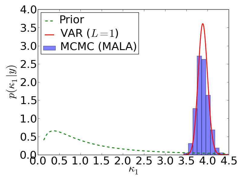
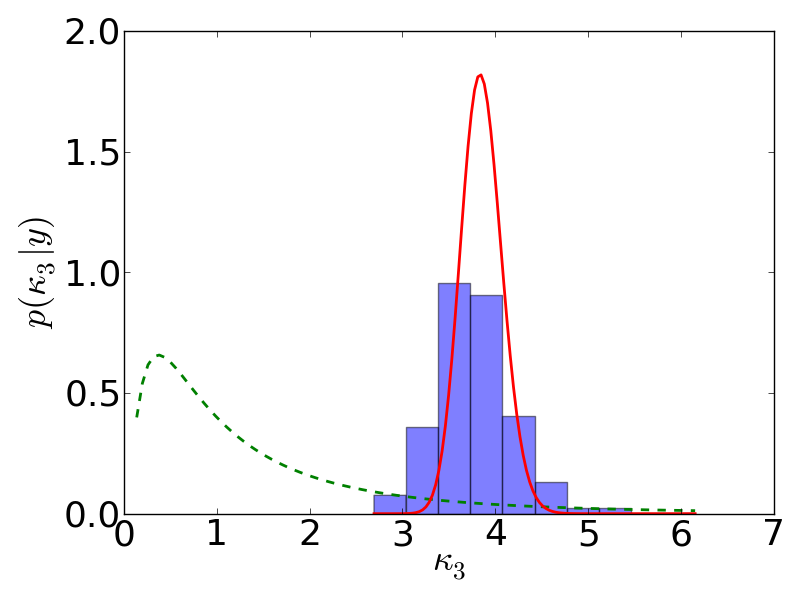
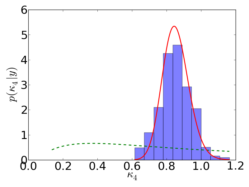
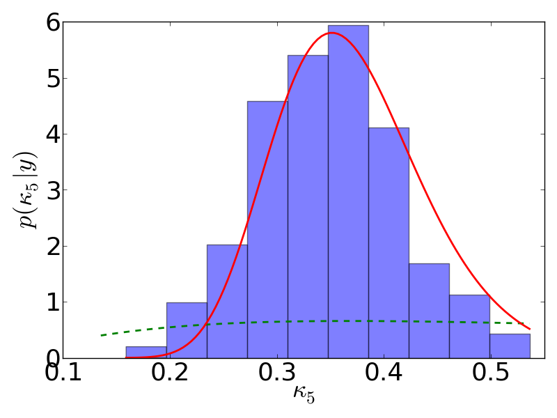
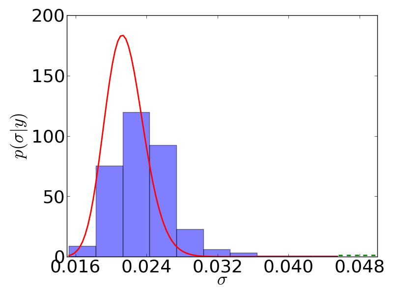
Figure 2: Reaction kinetic model: Comparison of the variational posterior (VAR ($L=1$)) of the scaled kinetic rate constants $\kappa_{i}$ as well as of the likelihood noise $\sigma$ to the MCMC (MALA) histograms of the same quantity. The prior probability density of each quantity is shown as a dashed green line.

We use the isotropic Gaussian likelihood defined in Eq. (2). It is further discussed in 0.A.4. The prior we assign to the parameter $\theta$ of the likelihood is:

$$p(\theta)=\mathcal{N}(\theta|-1,1).$$ (35)

Since the noise represented by $\theta$ is $\sigma=e^{\theta}$, this prior choice corresponds to a belief that the measurement noise is around $30$%.

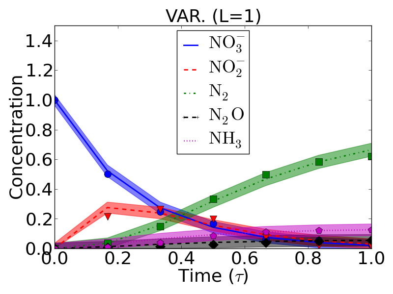
Figure 3: Reaction kinetic model: The ‘$\bullet$’, ‘$\triangledown$’, ‘$\square$’, ‘$\diamond$’, and ‘$\pentagon$’ signs indicate the scaled experimental measurements for $\mbox{NO}_{3}^{-}$, $\mbox{NO}_{2}^{-}$, $\mbox{N}_{2}$, $\mbox{N}_{2}\mbox{O}$, and $\mbox{NH}_{3}$, respectively. The lines and the shaded areas around them correspond to the median and $95\%$ credible intervals of the scaled concentration, $u_{i}$, as a function of the scaled time $\tau$. The left plot, shows the results obtained by approximating the posterior of the parameters via the variational approach. The right plot, shows the results obtained via MCMC (MALA).

We solve the problem using the variational approach as outlined in Algorithm 1. To approximate the posterior, we only use one Gaussian, $L=1$ in Eq. (15). We impose no bounds on $\boldsymbol{\mu}_{1}=\boldsymbol{\mu}\in\mathbb{R}^{d}$. However, we require that the diagonal elements $\sigma_{i}^{2}$ of the covariance matrix $\boldsymbol{\Sigma}_{1}=\boldsymbol{\Sigma}=\mbox{diag}\left(\sigma_{1},\dots,\sigma_{d}\right)$ are bounded below by $10^{-6}$ and above by $10^{2}$.

Table 2 compares the variational estimates of the scaled kinetic rate constants, $\xi$ (see Eq. (31)), and the logarithm of the likelihood noise, $\theta$ (see Eq. (2)), to the MCMC (MALA) estimates. We see that the mean of the two estimates are in close agreement, albeit the variational approach slightly underestimates the uncertainty of its prediction. However, notice that if we order the parameters in terms of increasing uncertainty, both methods yield the same ordering. Therefore, even though the numerical estimates of the uncertainty differ, the relative estimates of the uncertainty are qualitatively the same. It is worth mentioning at this point, that the variational approach uses only $37$ evaluations of the forward model. This is to be contrasted with the thousands of evaluations required so that the MCMC (MALA) estimates converge.

The variational approach with $L=1$ approximates the posterior of $\boldsymbol{\xi}$ and $\theta$ with one multivariate Gaussian distribution with a diagonal covariance. Therefore, the distribution of each one of the components is a Gaussian. Using Eqs. (31) and (29), it is easy to show that the kinetic rate constant $k_{i}$ follows a log-normal distribution with log-scale parameter $\mu_{i}-\log(180)$ and shape parameter $\sigma_{i}$. Similarly, we can show that the noise $\sigma=e^{\theta}$ follows a log-normal distribution with local-scale parameter $\mu_{d}$ and shape parameter $\sigma_{d}$. Using the percentiles of these lognormal distributions, we compute the median and the $95\%$ credible intervals of the kinetic rate constants $k_{i}$ and the noise $\sigma$. The results are shown in the third and fourth columns of table 3. They are in good agreement with the results found in [19] using a MCMC strategy (reproduced in the second column of the same table 3). An element of our analysis not found in [19] is the estimation of the measurement noise. Since $\sigma$ measures the noise of the scaled version of the data $\mathbf{y}$, we see (last line of table 3) that the measurement noise is estimated to be around 2.15%.

In figure 2, we compare the variational posterior (VAR ($L=1$)) of the scaled kinetic rate constants, $\kappa_{i}$, as well as of the noise of the likelihood, $\sigma$, to histograms of the same quantities obtained via MCMC (MALA). Once again, we confirm the excellent agreement between the two methods. In the same figure, we also plot the prior probability density we assigned to each parameter. The prior probability of $\sigma$ is practically invisible, because it picks at about $\sigma=0.30$. Given the big disparity between prior and posterior distributions, we see that the result is relatively insensitive to the priors we assign. If, in addition, we take into account that the measurement noise is estimated to be quite small, we conclude that Eq. (26) does a very good job of explaining the experimental observations.

Figure 3 shows the uncertainty in the scaled concentrations, $u_{i}$, as a function of scaled time, $\tau$, obtained by approximating the posterior of the parameters and compares them with the variational approach (left), to the MCMC (MALA) estimate. Again, we notice that the two plots are in very good agreement, albeit the variational approach seems to slightly underestimate the uncertainty.

3.2 Contaminant source identification

We now apply our methodology to a synthetic example of contaminant source identification. We are assuming that we have experimental measurements of contaminant concentrations at specific locations, and we are interested in estimating the location of the contamination source.

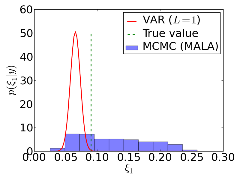
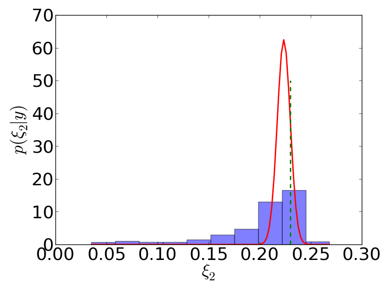
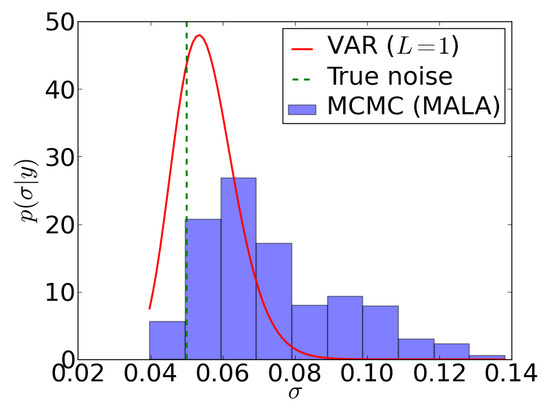
Figure 4: Contaminant source identification, first case: Comparison of the variational posterior (VAR ($L=1$)) of the source location $\boldsymbol{\xi}=(\xi_{1},\xi_{2})$ as well as of the likelihood noise $\sigma$ to the MCMC (MALA) histograms of the same quantities. The true value of each quantity is marked by a vertical, green, dashed line.

The concentration of the contaminant obeys the two-dimensional transport model described by a diffusion equation

$$\frac{\partial u}{\partial t}=\nabla^{2}u+g(t,\mathbf{x},\boldsymbol{\xi}),\;\mathbf{x}\in B,$$ (36)

where $B=[0,1]^{2}$ is the spatial domain and $g(t,\mathbf{x},\boldsymbol{\xi})$ is the source term. The source term is assumed to have a Gaussian:

$$g(t,\mathbf{s};\mathbf{x}_{s})=g_{0}e^{-\frac{|\mathbf{x}-\boldsymbol{\xi}|^{2}}{2\rho^{2}}}1_{[0,T_{s}]}(t),$$ (37)

where $g_{0}=\frac{1}{\pi\rho}$ is the strength of the contamination, $\rho=0.05$ is its spreadwidth, $T_{s}=0.3$ is the shutoff time parameter, and $\boldsymbol{\xi}$ is the source center. Therefore, $\boldsymbol{\xi}$ is the only parameter that needs to be identified experimentally. We impose homogeneous Neumann boundary conditions

$$\nabla\mathbf{u}\cdot\mathbf{n}=0,\;\mathbf{x}\in\partial B$$ (38)

and zero initial condition

$$\mathbf{u}(0,\mathbf{x},\boldsymbol{\xi})=0.$$ (39)

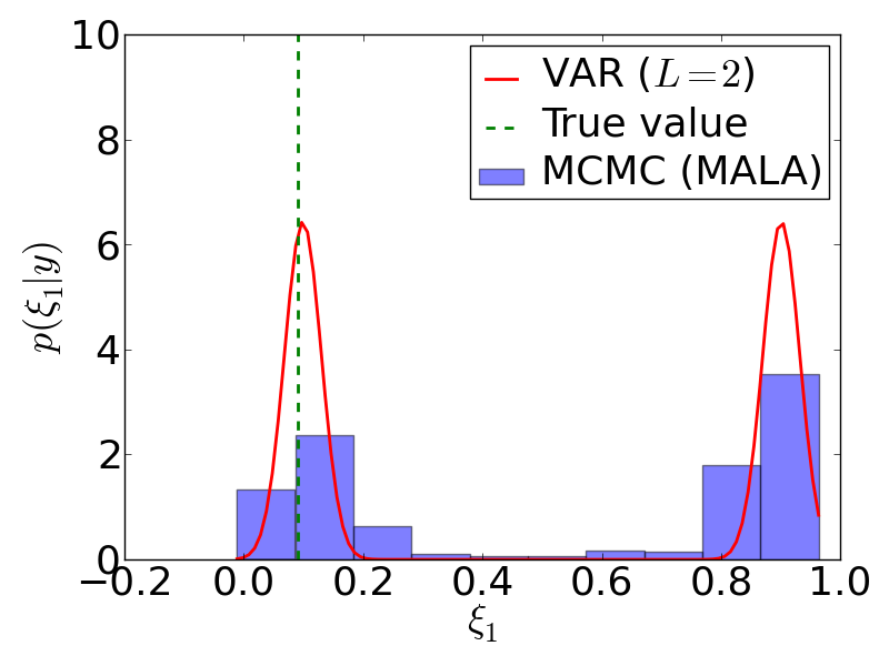
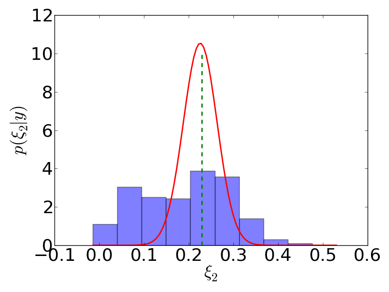
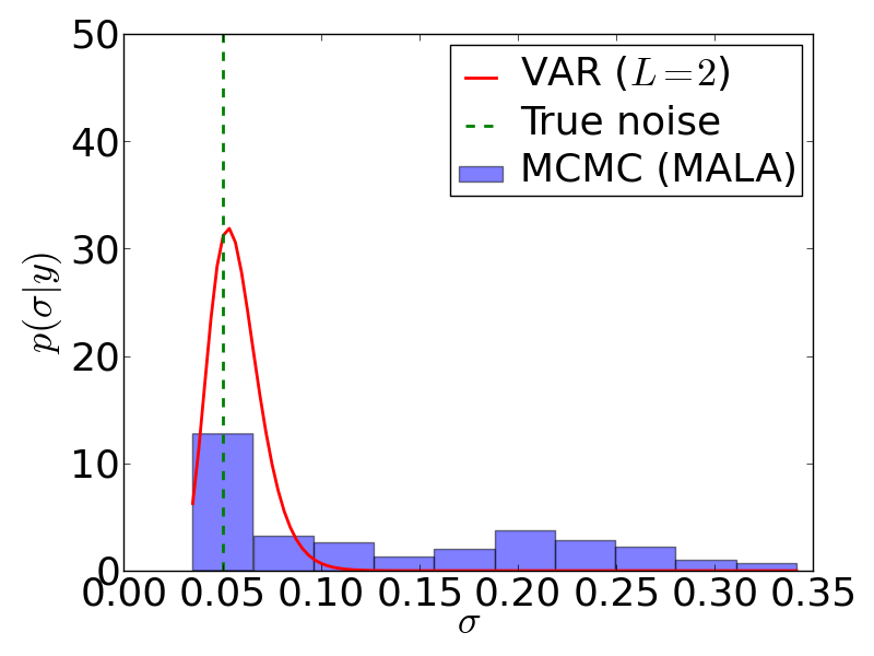
Figure 5: Contaminant source identification, second case: Comparison of the variational posterior (VAR ($L=1$)) of the source location $\boldsymbol{\xi}=(\xi_{1},\xi_{2})$ as well as of the likelihood noise $\sigma$ to the MCMC (MALA) histograms of the same quantities. The true value of each quantity is marked by a vertical, green, dashed line.

We consider two different scenarios. In the first one, measurements of $u(t,\mathbf{x},\boldsymbol{\xi})$ take place on the four corners of $B$. On the second one, measurements of $u(t,\mathbf{x},\boldsymbol{\xi})$ take place on the middle points of the upper and lower boundaries of $B$. The former results in a unimodal posterior for $\boldsymbol{\xi}$ and can be approximated with just one Gaussian. The latter results in a bimodal posterior for $\boldsymbol{\xi}$ and requires a mixture of two Gaussians. Eq. (36) is solved via a finite volume scheme implemented using the Python package Fipy[13]. The required gradients of the solution $u(t,\mathbf{x},\boldsymbol{\xi})$ are obtained by solving a series of PDE’s similar to Eq. (36) but with different source terms (see 0.A.6). In both scenarios, we generate synthetic observations, $\mathbf{y}$, by solving Eq. (36) on a $110\times 110$ grid, source $\boldsymbol{\xi}^{*}=(0.09,0.23)$, and adding Gaussian noise with standard deviation $\sigma^{*}=0.05$. For the forward evaluations needed during the calibration process we use a $25\times 25$ grid and we denote the corresponding solution by $\tilde{\mathbf{u}}(t,\mathbf{s};\boldsymbol{\xi})$. The prior we use for $\boldsymbol{\xi}$ is uniform,

$$p(\boldsymbol{\xi})\propto 1_{B}(\boldsymbol{\xi}),$$ (40)

the likelihood is given by Eq. (2), and the log-noise parameter $\theta$ of the likelihood has the same prior as the previous example (see Eq. (35)).

First case: Observations at the four corners

The synthetic data, $\mathbf{y}\in\mathbb{R}^{16}$ ($4$ sensors $\times$ $4$ measurements) are generated by sampling the $110\times 110$ solution, $u(t,\mathbf{x}):=u(t,\mathbf{x},\boldsymbol{\xi}^{*})$ at the four corners of $B$, and by adding Gaussian noise with $\sigma^{*}=0.05$:

$$\begin{array}[]{ccc}\mathbf{y}&=&\left(\begin{array}[]{c}u(t_{1},(0,0)),u(t_{1},(1,0)),u(t_{1},(0,1)),u(t_{1},(1,1)),\\ \vdots\\ u(t_{4},(0,0)),u(t_{4},(1,0)),u(t_{4},(0,1)),u(t_{4},(1,1))\end{array}\right)\\ &&+\;\mbox{noise}.\end{array}$$ (41)

The corresponding forward model generated by the $25\times 25$ solution, $\tilde{u}(t,\mathbf{x},\boldsymbol{\xi})$, is given by:

$$\mathbf{f}(\boldsymbol{\xi})=\left(\begin{array}[]{c}\tilde{u}(t_{1},(0,0),\boldsymbol{\xi}),\tilde{u}(t_{1},(1,0),\boldsymbol{\xi}),\tilde{u}(t_{1},(0,1),\boldsymbol{\xi}),\tilde{u}(t_{1},(1,1),\boldsymbol{\xi}),\\ \vdots\\ \tilde{u}(t_{4},(0,0),\boldsymbol{\xi}),\tilde{\mathbf{u}}(t_{4},(1,0),\boldsymbol{\xi}),\tilde{u}(t_{4},(0,1);\boldsymbol{\xi}),\tilde{u}(t_{4},(1,1),\boldsymbol{\xi})\end{array}\right).$$ (42)

Figure 4 compares the posteriors obtained via the variational approach with $L=1$ Gaussian in Eq. (15) to those obtained via MCMC (MALA). The true value of each parameter is indicated by a vertical, green, dashed line. It is worth noting at this point, that the variational approach required $48$ forward model evaluations as opposed to thousands required by MCMC (MALA). In real time, the variational approach took about 15 minutes on a single computational node, while the MCMC (MALA) required 3 days on the same node. Notice that the posterior cannot identify the true source exactly. This is due to the $5\%$ noise that we have added in the synthetic data. The result of such noise is always to broaden the posterior. We see that the variational approach does a good job in identifying an approximate location for the source $\boldsymbol{\xi}$ as well as estimating the noise level $\sigma$. However, we notice once again that it underestimates the true uncertainty.

Second case: Observations at the middle point of the upper and lower boundaries

The synthetic data, $\mathbf{y}\in\mathbb{R}^{8}$ ($2$ sensors $\times$ $4$ measurements) are generated by sampling the $110\times 110$ solution, $u(t,\mathbf{x}):=u(t,\mathbf{x},\boldsymbol{\xi}^{*})$ at the upper and lower boundaries of $B$, and by adding Gaussian noise with $\sigma^{*}=0.05$:

$$\begin{array}[]{ccc}\mathbf{y}&=&\left(\begin{array}[]{c}u(t_{1},(0.5,0)),u(t_{1},(0.5,1)),\\ \vdots\\ u(t_{4},(0.5,0)),u(t_{4},(0.5,1))\end{array}\right)\\ &&+\;\mbox{noise}.\end{array}$$ (43)

The corresponding forward model generated by the $25\times 25$ solution, $\tilde{u}(t,\mathbf{x},\boldsymbol{\xi})$, is given by:

$$\mathbf{f}(\boldsymbol{\xi})=\left(\begin{array}[]{c}\tilde{u}(t_{1},(0.5,0),\boldsymbol{\xi}),\tilde{u}(t_{1},(0.5,1),\boldsymbol{\xi}),\\ \vdots\\ \tilde{u}(t_{4},(0.5,0),\boldsymbol{\xi}),\tilde{\mathbf{u}}(t_{4},(0.5,1),\boldsymbol{\xi})\end{array}\right).$$ (44)

Figure 5 compares the posteriors obtained via the variational approach with $L=2$ Gaussians in Eq. (15) to those obtained via MCMC (MALA). The true value of each parameter is indicated by a vertical, green, dashed line. It is worth noting at this point, that the variational approach required only $62$ forward model evaluations. Using symmetry arguments, it is easy to show that data generated by solving Eq. (36) with a source located at $(\xi_{1},\xi_{2})$ look identical to the data that can be generated from a source located at $(1-\xi_{1},\xi_{2})$. As a result, the posterior distribution is bimodal. Therefore, we expect common MCMC methodologies to have a hard time dealing with this problem. The reason is that once the MCMC chain visits one of the modes, it is very unlikely that it will ever leave it to visit the other mode. In reality, it is impossible to visit the other mode unless a direct jump is proposed. The reason our MCMC (MALA) scheme works is because we have handpicked a proposal step that does allow for occasional jumps from one mode to the other. On the other hand, we see that the variational approach with $L=2$ Gaussians in Eq. (15) can easily deal with bimodal (or multimodal) posteriors. However, there are a few details that need to be mentioned here. Firstly, one needs to use an $L$ greater than or equal to the true number of modes of the posterior. Since, the latter is unknown, a little bit of experimentation would be required in a real problem. Secondly, even if the true $L$ is used, Algorithm 1 might still find fewer modes than the true number. For example, in our numerical experiments we have noticed that if $\boldsymbol{\mu}_{1}$ and $\boldsymbol{\mu}_{2}$ of Eq. (15) with $L=2$ are initially very close together, they are both attracted by the same mode. We believe that this is an artifact introduced by the Taylor approximation to the joint probability function $\mathcal{L}[q]$ (see Eq. (22) and Eq. (23)), and, in particular, of its local nature. In our example, a few random initializations of the $\boldsymbol{\mu}_{i}$’s are enough to guarantee the identification of both posterior modes.

4 Conclusions

We presented a novel approach to inverse problems that provides an optimization perspective to the Bayesian point of view. In particular, we used information theoretic arguments to derive an optimization problem that targets the estimation of the posterior within the the class of mixtures of Gaussians. The scheme proceeds by postulating that the “best” approximate posterior is the one that exhibits the minimum information loss (relative entropy) within the class of candidate posteriors. We showed how the minimization of the information loss is equivalent to the maximization of a lower bound to the evidence (normalization constant of the posterior). Since the derived lower bound was a computationally intractable quantity, we derived a crude approximation to it that requires the gradients of the forward model with respect to the input variables that we want to infer.

We demonstrated the efficacy of our method to solve inverse problems with just a few forward model evaluations in two numerical examples: 1) the estimation of the kinetic rate constants in a catalysis system, and 2) the identification of the contamination source in a simple diffusion problem. The performance of the scheme was compared to that of a state of the art MCMC technique (MALA) and was found to be satisfactory, albeit slightly underestimating the uncertainty. The scheme was able to solve both inverse problems with a fraction of the computational cost. In particular, our approach required around 50 forward model evaluations as opposed to the tens of thousands that are required by MCMC.

The variational approach seems to open up completely new ways of solving stochastic inverse problems. The scope of the approach is much wider than the particular techniques used in this paper. Just as a indication, the following are some of the research directions that we plan to pursue in the near future: 1) Derive alternative -more accurate- approximations to the lower bound of the evidence; 2) Experiment with dimensionality reduction ideas that would allow us to carry out the variational optimization in high-dimensional problems; 3) Derive stochastic algorithms for maximizing the lower bound without invoking any approximations. We believe that the variational approach has the potential of making stochastic inverse problems solvable with only a moderate increase in the computational cost as compared to classical approaches.

Appendix 0.A Computation of $\mathcal{F}_{a}[q]$ and its gradient

Algorithm 1 requires the evaluation of the gradient of the approximate ELBO of Eq. (24) with respect to all the parameters of the Gaussian mixture $q(\boldsymbol{\omega})$ of Eq. (15). That is, we must be able to evaluate

$$\mathcal{F}_{a}[q] = \mathcal{H}_{0}[q]+\mathcal{L}_{a}[q],$$ (45)

$$\frac{\partial}{\partial\beta}\mathcal{F}_{a}[q] = \frac{\partial}{\partial\beta}\mathcal{H}_{0}[q]+\frac{\partial}{\partial\beta}\mathcal{L}_{a}[q],$$ (46)

for $\beta=w_{i},\mu_{ij}=(\boldsymbol{\mu}_{i})_{j}$, $\Sigma_{ijk}=(\boldsymbol{\Sigma}_{i})_{jk}$ for $i=1,\dots,L$, and $j,k=1,\dots,d$ and $a=0,2$.

0.A.1 Computation of $\mathcal{H}_{0}[q]$ and its gradient

The computations relative to $\mathcal{H}_{0}[q]$ are:

$$\mathcal{H}_{0}[q] = -\sum_{i=1}^{L}w_{i}\log(q_{i}),$$ (47)

$$\frac{\partial}{\partial w_{i}}\mathcal{H}_{0}[q] = -\log(q_{i})-\sum_{r=1}^{L}\frac{w_{r}N_{ri}}{q_{r}},$$ (48)

$$\frac{\partial}{\partial\mu_{ij}}\mathcal{H}_{0}[q] = -w_{i}\sum_{r=1}^{L}w_{r}N_{ri}A_{rij}\left(\frac{1}{q_{i}}+\frac{1}{q_{r}}\right),$$ (49)

$$\frac{\partial}{\partial\Sigma_{ijk}}H_{0}[q] = \frac{1}{2}w_{i}\sum_{r=1}^{L}w_{r}N_{ri}B_{rijk}\left(\frac{1}{q_{i}}+\frac{1}{q_{r}}\right),$$ (50)

where, in order to simplify the notation, we have used the following intermediate quantities:

$$N_{ri} = \mathcal{N}\left(\boldsymbol{\mu}_{r}|\boldsymbol{\mu}_{i},\boldsymbol{\Sigma}_{r}+\boldsymbol{\Sigma}_{i}\right),$$ (51)

$$q_{i} = \sum_{r=1}^{L}w_{r}N_{ri},$$ (52)

$$A_{rij} = \sum_{s=1}^{d}\left(\boldsymbol{\Sigma}_{r}+\boldsymbol{\Sigma}_{i}\right)^{-1}_{js}\left(\mu_{rs}-\mu_{is}\right),$$ (53)

$$B_{rijk} = \left(\boldsymbol{\Sigma}_{r}+\boldsymbol{\Sigma}_{i}\right)^{-1}_{jk}+A_{rij}A_{rik}.$$ (54)

0.A.2 Computation of $\mathcal{L}_{a}[q]$ and its gradients

The computations relative to the $\mathcal{L}_{a}[q]$ part are:

$$\mathcal{L}_{0}[q] = \sum_{i=1}^{L}w_{i}C_{i},$$ (55)

$$\frac{\partial}{\partial w_{i}}\mathcal{L}_{0}[q] = C_{i},$$ (56)

$$\frac{\partial}{\partial\mu_{ij}}\mathcal{L}_{0}[q] = D_{ij},$$ (57)

$$\frac{\partial}{\partial\Sigma_{ijk}}\mathcal{L}_{0}[q] = 0,$$ (58)

$$\mathcal{L}_{2}[q] = \mathcal{L}_{0}[q]+\frac{1}{2}\sum_{i=1}^{L}w_{i}\sum_{j,k=1}^{d}\Sigma_{ijk}E_{ijk},$$ (59)

$$\frac{\partial}{\partial w_{i}}\mathcal{L}_{2}[q] = \frac{\partial}{\partial w_{i}}\mathcal{L}_{0}[q]+\frac{1}{2}\sum_{j,k=1}^{d}\Sigma_{ijk}E_{ijk},$$ (60)

$$\frac{\partial}{\partial\Sigma_{ijk}}\mathcal{L}_{2}[q] = \frac{\partial}{\partial\Sigma_{ijk}}\mathcal{L}_{0}[q]+\frac{1}{2}w_{i}E_{ijk},$$ (61)

where, in order to simplify the notation, we have used the following intermediate quantities:

$$J(\boldsymbol{\omega}) = \log p(\mathbf{y},\boldsymbol{\omega})=\log p(\mathbf{y}|\boldsymbol{\omega})+\log p(\boldsymbol{\omega}),$$ (62)

$$C_{i} = J(\boldsymbol{\mu}_{i}),$$ (63)

$$D_{ij} = \frac{\partial}{\partial\omega_{j}}J(\boldsymbol{\mu}_{i}),$$ (64)

$$E_{ijk} = \frac{\partial^{2}}{\partial\omega_{j}\omega_{k}}J(\boldsymbol{\mu}_{i}).$$ (65)

We do not provide the derivatives of $\mathcal{L}_{2}[q]$ with respect to $\mu_{ijk}$ because they are not needed in Algorithm 1. The joint probability function $J(\boldsymbol{\omega})$ of Eq. (62) depends on the details of the likelihood, the prior, and the underlying forward model. We discuss the computation of Eqs. (62), (64), and (65) in 0.A.3.

0.A.3 Computing the derivatives of $J(\boldsymbol{\omega})$

In this section, we show how the gradient of the forward model appears through the differentiation of the joint probability density $J(\boldsymbol{\omega})$ of Eq. (62). Recall (see beginning of section 2) that $\boldsymbol{\omega}=(\boldsymbol{\xi},\boldsymbol{\theta})$, where $\boldsymbol{\xi}$ are the parameters of the forward model $\mathbf{f}(\boldsymbol{\xi})\in\mathbb{R}^{m}$, and $\boldsymbol{\theta}$ the parameters of the likelihood function of Eq. (1). Therefore, let us write:

$$J(\boldsymbol{\omega})=J(\boldsymbol{\xi},\boldsymbol{\theta}) = L(\mathbf{y},\mathbf{f}(\boldsymbol{\xi}),\boldsymbol{\theta})+P_{\xi}(\boldsymbol{\xi})+P_{\theta}(\boldsymbol{\theta}),$$ (66)

$$L(\mathbf{y},\mathbf{f}(\boldsymbol{\xi}),\boldsymbol{\theta}) = \log p(\mathbf{y}|\mathbf{f}(\boldsymbol{\xi}),\boldsymbol{\theta}),$$ (67)

$$P_{\xi}(\boldsymbol{\xi}) = \log p(\boldsymbol{\xi}),$$ (68)

$$P_{\theta}(\boldsymbol{\theta}) = \log p(\boldsymbol{\theta}).$$ (69)

Using the chain rule, we have:

$$\frac{\partial J}{\partial\xi_{j}} = \sum_{s=1}^{d_{y}}\frac{\partial L}{\partial f_{s}}\frac{\partial f_{s}}{\partial\xi_{j}}+\frac{\partial P_{\xi}}{\partial\xi_{j}},$$ (70)

$$\frac{\partial J}{\partial\theta_{j}} = \frac{\partial L}{\partial\theta_{j}}+\frac{\partial P_{\theta}}{\partial\theta_{j}},$$ (71)

$$\frac{\partial^{2}J}{\partial\xi_{j}\partial\xi_{j}} = \sum_{s,r=1}^{d_{y}}\frac{\partial^{2}L}{\partial f_{r}\partial f_{s}}\frac{\partial f_{r}}{\partial\xi_{k}}\frac{\partial f_{s}}{\partial\xi_{j}}+\sum_{s=1}^{d_{y}}\frac{\partial L}{\partial f_{s}}\frac{\partial^{2}f_{s}}{\partial\xi_{j}\partial\xi_{k}}+\frac{\partial^{2}P_{\xi}}{\partial\xi_{j}\partial\xi_{k}},$$ (72)

$$\frac{\partial^{2}J}{\partial\theta_{i}\partial\theta_{j}} = \frac{\partial^{2}L}{\partial\theta_{i}\partial\theta_{j}}+\frac{\partial^{2}P_{\xi}}{\partial\theta_{i}\partial\theta_{j}},$$ (73)

$$\frac{\partial^{2}J}{\partial\xi_{j}\partial\theta_{k}} = \sum_{s=1}^{d_{y}}\frac{\partial^{2}L}{\partial\theta_{k}\partial f_{s}}\frac{\partial f_{s}}{\partial\xi_{j}}.$$ (74)

Therefore, the Jacobian and the Hessian of the forward model are required. However, as is obvious by close inspection of Eqs. (59), (60), and (61), if the covariance matrices of the mixture $q(\boldsymbol{\omega})$ of Eq. (15) are diagonal, then only the diagonal elements of the Hessian of the forward model are essential. This is the approach we follow in our numerical examples.

0.A.4 Isotropic Gaussian likelihood

In both our numerical examples, we use the isotropic Gaussian likelihood defined in Eq. (2). Its logarithm is:

$$L(\mathbf{y},\mathbf{f}(\boldsymbol{\xi}),\theta)=\log\mathcal{N}\left(\mathbf{y}|\mathbf{f}(\boldsymbol{\xi}),e^{2\theta}\mathbf{I}\right).$$ (75)

The required gradients are:

$$\frac{\partial L}{\partial f_{r}} = e^{-2\theta}\left(y_{r}-f_{r}(\boldsymbol{\xi})\right),$$

$$\frac{\partial L}{\partial\theta} = e^{-\theta}\left(\parallel\mathbf{y}-\mathbf{f}(\boldsymbol{\xi})\parallel_{2}^{2}e^{-2\theta}-d_{\xi}\right),$$

$$\frac{\partial^{2}L}{\partial\theta^{2}} = e^{-\theta}\left(d_{\xi}-3\parallel\mathbf{y}-\mathbf{f}(\boldsymbol{\xi})\parallel_{2}^{2}e^{-2\theta}\right),$$

$$\frac{\partial^{2}L}{\partial f_{r}\partial f_{s}} = -e^{-2\theta},$$

$$\frac{\partial^{2}L}{\partial\theta\partial f_{r}} = -2e^{-3\theta}\left(y_{r}-f_{r}(\boldsymbol{\xi})\right).$$

0.A.5 Derivatives of a dynamical system

Assume that $\mathbf{u}(t,\boldsymbol{\xi})\in\mathbb{R}^{d_{u}}$ is the solution of the following initial value problem:

$$\begin{array}[]{cc}\dot{\mathbf{u}}&=\mathbf{g}(\mathbf{u},t,\boldsymbol{\xi}),\\ \mathbf{u}(0)&=\mathbf{u}_{0}(\boldsymbol{\xi}),\end{array}$$ (76)

where $\boldsymbol{\xi}\in\mathbb{R}^{d_{\xi}}$ are parameters. Using the chain rule, one can show that the derivatives of $\mathbf{u}(t,\boldsymbol{\xi})$ with respect to $\boldsymbol{\xi}$, $v_{ij}=\frac{\partial u_{i}}{\partial\xi_{j}}$, satisfy the following initial value problem:

$$\begin{array}[]{cc}\dot{v}_{ij}&=\sum_{r=1}^{d_{u}}\frac{\partial g_{i}}{\partial u_{r}}v_{rj}+\frac{\partial g_{i}}{\partial\xi_{j}},\\ v_{ij}(0)&=\frac{\partial u_{0}}{\partial\xi_{j}}.\end{array}$$ (77)

The second derivatives $w_{ijk}=\frac{\partial^{2}u_{i}}{\partial\xi_{j}\partial\xi_{k}}$, satisfy the following initial value problem:

$$\begin{array}[]{cc}\dot{w}_{ijk}&=\sum_{r=1}^{d_{u}}\frac{\partial g_{i}}{\partial u_{r}}w_{rjk}+\sum_{r,s=1}^{d_{u}}\frac{\partial^{2}g}{\partial u_{r}\partial u_{s}}v_{rj}v_{sk}+\frac{\partial^{2}g_{i}}{\partial\xi_{j}\partial\xi_{k}},\\ w_{ijk}(0)&=\frac{\partial^{2}u_{0}}{\partial\xi_{j}\partial\xi_{k}}.\end{array}$$ (78)

The numerical strategy for solving these systems is quite simple. First, we solve Eq. (76) using an explicit runge-kutta method of order (4)5. Then, we use the solution as forcing in Eq. (77) to find the gradient. Finally, both the solution and the gradient are used as forcing in Eq. (78).

0.A.6 Derivatives of the diffusion equation

Let $u(t,\mathbf{s},\boldsymbol{\xi})\in\mathbb{R}^{d_{u}}$ be the solution of the partial differential equation Eq. (36). The derivatives $v_{i}=\frac{\partial u}{\partial\xi_{i}}$ satisfy the partial differential equation

$$\frac{\partial v_{i}}{\partial t}=\nabla^{2}v_{i}+\frac{\partial g(t,\mathbf{x},\boldsymbol{\xi})}{\partial\xi_{i}}.$$ (79)

Similarly the second derivatives $w_{ij}=\frac{\partial^{2}u}{\partial\xi_{i}\partial\xi_{j}}$ satisfy

$$\frac{\partial w_{ij}}{\partial t}=\nabla^{2}w_{ij}+\frac{\partial^{2}g(t,\mathbf{x},\boldsymbol{\xi})}{\partial\xi_{i}\partial\xi_{j}}.$$ (80)

Equations (36), (79),  and (80) are solved numerically using the same space- and time-discretization and the finite volume solver provided by FiPy [13]. The only thing that changes is the source term.

References

References

- [1] Yves F. Atchadé. An adaptive version for the metropolis adjusted Langevin algorithm with a truncated drift. Methodology and Computing in Applied Probability, 8:235–254, 2006.
- [2] I. Bilionis and P.S. Koutsourelakis. Free energy computations by minimization of Kullback–Leibler divergence: An efficient adaptive biasing potential method for sparse representations. Journal of Computational Physics, 231(9):3849–3870, 2012.
- [3] I Bilionis and N Zabaras. Solution of inverse problems with limited forward solver evaluations: a bayesian perspective. Inverse Problems, 30(1):015004, 2014.
- [4] Ilias Bilionis, Beth A. Drewniak, and Emil M. Constantinescu. Crop physiology calibration in CLM. Geoscientific Model Development (under review), 2014.
- [5] Ilias Bilionis and Nicholas Zabaras. A stochastic optimization approach to coarse-graining using a relative-entropy framework. The Journal of Chemical Physics, 138(4):–, 2013.
- [6] Richard H. Byrd, Peihuang Lu, Jorge Nocedal, and Ciyou Zhu. A Limited Memory Algorithm for Bound Constrained Optimization, 1995.
- [7] Peng Chen, Nicholas Zabaras, and Ilias Bilionis. Uncertainty Propagation using Infinite Mixture of Gaussian Processes and Variational Bayesian Inference, in press. Journal of Computational Physics, 2014.
- [8] A. Fichtner. Full Seismic Waveform Modelling and Inversion. Advances in Geophysical and Environmental Mechanics and Mathematics. Springer, 2010.
- [9] Andreas Fichtner. Full Seismic Waveform Modelling and Inversion, 2011.
- [10] Charles W. Fox and Stephen J. Roberts. A tutorial on variational Bayesian inference. Artificial Intelligence Review, 38(2):85–95, June 2011.
- [11] Samuel Gershman, Matthew D. Hoffman, and David M. Blei. Nonparametric variational inference. CoRR, abs/1206.4665, 2012.
- [12] A. Griewank and A. Walther. Evaluating Derivatives: Principles and Techniques of Algorithmic Differentiation, Second Edition. SIAM e-books. Society for Industrial and Applied Mathematics (SIAM, 3600 Market Street, Floor 6, Philadelphia, PA 19104), 2008.
- [13] J.E. Guyer, D. Wheeler, and J.A. Warren. Fipy: Partial differential equations with python. Computing in Science and Engineering, 11(3):6–15, 2009.
- [14] W. K. Hastings. Monte Carlo sampling methods using Markov chains and their applications. Biometrika, 57(1):97–109, 1970.
- [15] Mary C. Hill and Claire R. Tiedeman. Effective Groundwater Model Calibration: With Analysis of Data, Sensitivities, Predictions, and Uncertainty. Wiley, 2006.
- [16] Marco F. Huber, Tim Bailey, Hugh Durrant-Whyte, and Uwe D. Hanebeck. On entropy approximation for gaussian mixture random vectors. In Proceedings of the 2008 IEEE International Conference on Multisensor Fusion and Integration for Intelligent Systems (MFI), Seoul, Südkorea, August 2008.
- [17] E.T. Jaynes and G.L. Bretthorst. Probability Theory: The Logic of Science. Cambridge University Press, 2003.
- [18] Eugenia Kalnay. Atmospheric Modeling, Data Assimilation and Predictability. Cambridge University Press, 1 edition, December 2002.
- [19] I Katsounaros, M Dortsiou, C Polatides, S Preston, T Kypraios, and G Kyriacou. Reaction pathways in the electrochemical reduction of nitrate on tin. Electrochimica Acta, 71:270–276, 2012.
- [20] M.C. Kennedy and A. O’Hagan. Bayesian calibration of computer models. Journal of the Royal Statistical Society: Series B (Statistical Methodology), pages 425–464, 2001.
- [21] S. Kullback and R. A. Leibler. On Information and Sufficiency. The Annals of Mathematical Statistics, 22(1):79–86, 1951.
- [22] Youssef Marzouk and Dongbin Xiu. A Stochastic Collocation Approach to Bayesian Inference in Inverse Problems. Communications in Computational Physics, 6(4):826–847, 2009.
- [23] Geoffrey McLachlan and David Peel. Finite Mixture Models. John Wiley & Sons, 2004.
- [24] N. Metropolis, A. W. Rosenbluth, M. N. Rosenbluth, A. H. Teller, and E. Teller. Equation of state calculations by fast computing machines. The Journal of Chemical Physics, 21(6):1087–1092, 1953.
- [25] Ionel Navon M. Data assimilation for numerical weather prediction: A review. In SeonK. Park and Liang Xu, editors, Data Assimilation for Atmospheric, Oceanic and Hydrologic Applications, pages 21–65. Springer Berlin Heidelberg, 2009.
- [26] R.-E. Plessix. A review of the adjoint-state method for computing the gradient of a functional with geophysical applications. Geophysical Journal International, 167(2):495–503, November 2006.
- [27] Herbert Robbins and Sutton Monro. A stochastic approximation method. The Annals of Mathematical Statistics, 22(3):400–407, 09 1951.
- [28] A. Tarantola. Inverse Problem Theory and Methods for Model Parameter Estimation. Society for Industrial and Applied Mathematics (SIAM, 3600 Market Street, Floor 6, Philadelphia, PA 19104), 2005.