Frequency-dependent attenuation and elasticity in unconsolidated earth materials: effect of damping
Abstract
We use the Discrete Element Method (DEM) to understand the underlying attenuation mechanism in granular media, with special applicability to the measurements of the so-called effective mass developed earlier. We consider that the particles interact via Hertz-Mindlin elastic contact forces and that the damping is describable as a force proportional to the velocity difference of contacting grains. We determine the behavior of the complex-valued normal mode frequencies using 1) DEM, 2) direct diagonalization of the relevant matrix, and 3) a numerical search for the zeros of the relevant determinant. All three methods are in strong agreement with each other. The real and the imaginary parts of each normal mode frequency characterize the elastic and the dissipative properties, respectively, of the granular medium. We demonstrate that, as the interparticle damping, , increases, the normal modes exhibit nearly circular trajectories in the complex frequency plane and that for a given value of they all lie on or near a circle of radius centered on the point in the complex plane, where . We show that each normal mode becomes critically damped at a value of the damping parameter , where is the (real-valued) frequency when there is no damping. The strong indication is that these conclusions carry over to the properties of real granular media whose dissipation is dominated by the relative motion of contacting grains. For example, compressional or shear waves in unconsolidated dry sediments can be expected to become overdamped beyond a critical frequency, depending upon the strength of the intergranular damping constant.
INTRODUCTION
An important challenge in the development of a hydrocarbon reservoir is optimizing well completion and production. After placing a well, sonic well logging techniques characterize the subsurface at high resolution in the immediate vicinity of a borehole. For a given strata, the acoustic properties depend on many characteristics (composition, structure, porosity) and conditions (stress, temperature, pore fluid). In the soft unconsolidated formations of interest in the present study, sonic measurements are further complicated by nonlinear effects arising from heterogeneities, inhomogeneous stress distributions, and dissipation due to fluid flow (Domenico, 1977; O‘Connell and Budiansky, 1977; Digby, 1981; Winkler, 1983; Walton, 1987; Chen et al., 1988; Goddard, 1990; de Gennes, 1996; Behringer an Jenkins, 1997; Norris and Johnson, 1997; Johnson et al., 1998; Guyer and Johnson, 1999; Makse et al., 1999). These nonlinearities have important effects on the dynamics of unconsolidated media as reviewed by Guyer and Johnson (1999) and Johnson et al. (1996). Therefore, coupled with a representative model of the granular medium (Goddard, 1990; Guyer and Johnson, 1999; Domenico, 1977; Winkler, 1983; Behringer and Jenkins, 1997; Norris and Johnson, 1997) sonic wave propagation can be utilized to characterize subsurface conditions and elucidate active mechanisms. In turn, this information can be utilized during well completion and production. Another important effect of non-linearities is to cause dispersion in the system as studied in Johnson et al. (1996) and Guyer and Johnson (1999).
The motivation of the present study is to develop theoretical and numerical tools to study the acoustic and dissipative properties of unconsolidated granular materials. Our findings can then be employed to a) improve the interpretation of sonic logging measurements, and (b) to optimize granular media for the dissipation of acoustic energy. First, we utilize the Discrete Element Methods (DEM) to test the theory for the effective mass of discrete systems as outlined in Valenza and Johnson (2012). We utilize this DEM and analytical framework to calculate the frequency-dependent effective mass of unconsolidated granular media held in a cup, and study the effect of interparticle damping on the normal modes in the system.
Previous work on the normal modes of unconsolidated granular materials (Alexander, 1998; O‘Hern et al., 2003; Silbert at al., 2005; Somfai et al., 2007; Wyart et al., 2005a,b) have studied the vibrational density of states of a granular system as the external applied pressure is diminished and the volume fraction of the system decreases towards the point of random close packing (RCP), i.e., when the granular medium is a fragile unconsolidated formation (Makse et al., 2000) and (O‘Hern et al., 2003). However, these previous studies have not considered the important effect of attenuation on the normal modes. Attenuation plays a crucial role in governing the dynamic response of real system. Thus, interpretation of any experiment and acoustic logging needs to take into account the dissipative nature of granular matter.
In a previous study we have focused on the stress-dependent dissipative characteristics of the granular medium (Hu et al., 2014). The effect of attenuation at the grain-grain contacts has been also studied experimentally and theoretically in Valenza and Johnson (2012). Here, we test those theoretical developments with Discrete Element Methods (DEM) (Cundall, 1979) with a particular focus on the low-frequency modes in the effective mass of granular materials. We further develop this theoretical basis for granular systems in order to investigate the dependence of the normal modes on the damping mechanism at the interparticle contact. An area of primary focus is the consequences of assuming the elastic and damping matrices commute.
The paper is organized as follows: First we introduce the concept of the effective mass and then we review specific relevant theoretical results, in particular the relation between the effective mass and the normal modes of vibration in the system. In the special case that the damping matrix and the stiffness matrix are proportional to each other with proportionality , we derive properties of the trajectories of the normal mode frequencies, in the complex plane, as a function of . Next, we outline the DEM computational technique as well as the eigenvalue-eigenvector technique with which we compute the main results of this paper. Those results are analyzed in detail in view of the previously mentioned exact and approximate results and we conclude with our summarizing remarks.
EFFECTIVE MASS OF A GRANULAR MEDIUM
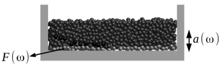
The effective mass of the granular medium in a cup of mass vibrating with frequency is defined as (Hsu et al., 2009):
| (1) |
For each frequency , is determined by measuring the force necessary to displace the cup and, is the associated acceleration. The system is schematically explained in Fig. 1. Experimentally, both quantities are recorded in the frequency domain after waiting a short stabilization period of a few seconds. Then, equation 1 is employed to construct . In general, is complex-valued and reflects the partially in-phase and out-of-phase motion of the individual grains relative to the cup motion. and characterize the ensemble averaged elastic and dissipative capacity of the material in a simplified continuum with negligible boundary effects (see for instance Henann et al. (2013). An ideal example is provided by a low viscosity liquid where the dimensions of the cup are much larger than the viscous skin depth across the experimental frequency band; In this case the effective mass resonates at odd-multiples of wavelength of the longitudinal wave in the medium (Hsu et al., 2009). In fact, the dominant low frequency normal modes in a granular medium exhibit similar scaling behavior. However, the scaling of the modes in a confined granular medium is effected by the preparation protocol, and boundary condition (Henann et al., 2013).
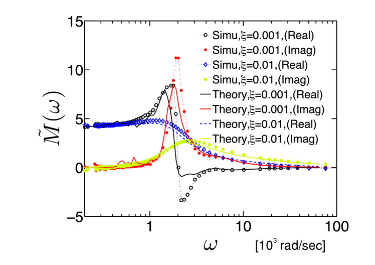
The imaginary part of the frequency dependent effective mass in a granular medium is roughly proportional to the frequency dependent attenuation in the system. This dissipation can be due to solid contact friction (asperities, material plasticity, etc.) or wetting dynamics from liquid bridges or films between grains. Figure 2 shows the results of a frequency sweep of the real () and imaginary () components of the effective mass obtained with DEM for packings under gravity with the indicated damping coefficients (DEM procedure outlined below). These results are qualitatively similar to those determined experimentally, and reported in Hsu et al. (2009) and Valenza and Johnson (2012). Here, we adapt the DEM technique to obtain the low-frequency modes in the region of interest. In a manner analogous to that achieved experimentally in Valenza and Johnson (2012) we use DEM to test the effect of interparticle damping on the dynamics of discrete systems.
PREVIOUS THEORETICAL RESULTS
Hertz-Mindlin interparticle force law
We consider a granular medium made of spherical particles interacting via Hertz-Mindlin contact forces and dissipative forces at the contact point. Our technique is generalizable, however, to nonspherical particles (Baule, et al., 2013; Baule and Makse, 2014). The normal component of the contact force between any two contacting particles with radius is the Hertz force (Landau and Lifschitz, 1970; Johnson, 1985) derived as:
| (2) |
where the normal deformation (1/2 the overlap between the spheres) between the neighboring grains is , are the position vectors, and is the normal spring constant. The latter is defined in terms of the corresponding material properties. The normal elastic constant is where is the shear modulus, and is the Poisson’s ratio of the material from which the grains are made.
The tangential Mindlin force between neighboring grains in contact is (Shafer et al., 1996):
| (3) |
where is the tangential spring constant, and the variable is defined such that the relative shear displacement between the two grain centers is .
In addition to these elastic forces we consider the effects of intergranular damping which are manifest here as forces proportional to the difference between the velocity values of two contacting grains. The general linearized form is and .
Finally, Coulomb friction with interparticle friction coefficient imposes at every contact. The experimental signature of this effect is that if the amplitude of vibration is large enough that adjacent grains slide against each other the measured effective mass becomes amplitude dependent. The previously cited experiments carefully avoided this situation by sticking to low amplitude vibrations. Accordingly, in the present article we shall assume either that there is no relative tangential slip between grains (perfect stick) or that there is no tangential force at all (perfect slip), as the case may be.
We are interested in the linear response of the granular system to infinitesimal perturbations. Therefore we consider the linearized forms of the above equations, ie, we use the Hertz-Mindlin force law linearized about the static value of the normal compression of contacts. The resulting elastic stiffness is the slope of the force law evaluated at (eg. equation 2 for the normal component) and equation 3 for the transverse component:
| (4) |
and
| (5) |
Our goal here is to understand the effects of dissipation when, for instance the particles are coated with a viscous fluid, such as described in the experiments of Valenza and Johnson (2012). The dissipation is mainly due to the ’squirt flow’ in liquid bridges at the particle contacts. We shall assume for simplicity that the damping constants are independent of the particle deformation and are therefore the same for all particles that are in contact. It shall prove to be convenient to write the damping forces as
| (6) |
and
| (7) |
where the overbar signifies an average over all non-zero contacts and , which has the dimensions of time, will be our control parameter. It is a stand-in for the viscosity of the fluid at the grain-grain contacts.
Theory of normal modes
In a typical experiment or simulation, the grains are settled in a cup that moves sinusoidally with magnitude , taken in the direction. We denote as the uniaxial displacement of the cup. In the analogous physical experiments (Hsu et al., 2009) is less than m, at least three orders of magnitude smaller than . This assures that the external displacement is smaller than the static compression at the grain contacts. Therefore, we take all to be infinitesimal, and utilize the linear equation of motion for the -th particle with mass to describe the system dynamics. The coupled equations of motion for the degrees of freedom in a system of particles is written as [see Valenza and Johnson (2012) and Hu et al. (2014) for details]:
| (8) |
where and label each of the degrees of freedom in the problem. The vector accounts for the set of particle displacements and particle rotations. The dynamical matrix in the frequency domain can be written as,
| (9) |
Here the mass matrix has elements , with the identity matrix if the particles interact via central forces only (frictionless), and it contains the moment of inertia for rotating particles interacting via tangential forces. Each term in accounts for the inertial term, the dissipative matrix , and elastic matrix , defined at the contact between particles and , respectively. The elements of the elastic matrix follow from the Hertz-Mindlin stiffness constants for infinitesimal displacement, equations 4 and 5. It is convenient to write this matrix for a given pair of grains and that are in contact as
| (10) |
where denotes the direction of the normal displacement along the contact point and we are using dyadic notation. Similarly, the damping matrix follows from equations 6 and 7 and may be written as
| (11) |
If the particles, and , are not in contact (), we set both and . In equation 8 is the generalized spring constant connecting a particle to the walls of the cup which moves oscillatory in the direction with amplitude .
Inverting the matrix we obtain the effective mass as has been shown in our previous work (Valenza and Johnson, 2012):
| (12) |
This equation expresses the relation between the effective mass and the normal mode spectrum. The peaks observed in the effective mass (Fig. 2), , are due to the set of normal modes, , that are a solution to equation 8 when there is no forcing by the cup, , i.e.,
| (13) |
Thus, the normal modes, , are those eigenvectors of for which the corresponding eigenvalue is zero, and they occur at specific complex-valued frequencies, .
EIGENVALUE TRAJECTORIES AS A FUNCTION OF DAMPING
While previous theoretical studies have considered the undamped modes of frictionless systems (Wyart et al., 2005a,b), the interpretation of the effective mass data from experiments or sonic logging data necessitates a formalism that considers damping and rotational modes that are indigenous in to real granular matter. Our formalism thus generalizes previous results valid for frictionless undamped systems to more realistic granular materials consisting of dissipative interactions with tangential forces.
Equation 12 implies that is the resonance frequency when has at least one zero eigenvalue or the determinant of is equal to zero. When , the resonance frequency is a complex number and the imaginary part is relevant to the attenuative properties of the granular system. Here, we study the effect of interparticle damping, , on the resonant modes .
We are interested in the complete set of complex valued normal modes that satisfy equation 13. For these modes, using some results from Caughey (1960) and Hu et al. (2014) we can rewrite equation 13 in the frequency domain as:
| (14) |
Here we have defined: , and , provided that the matrix is positive definite, we can always find .
It is obvious from their definitions, equations 10 and 11, that the matrices K and B do not commute. It shall prove to be informative to explore the consequences of assuming not only that they commute but that they are proportional to each other, viz:
| (15) |
The distribution of normal stiffness is directly related to the distribution of interparticle normal forces via the distribution of deformation . Such a force distribution is well known to display an exponential tail and to be relatively homogenous (Makse et al., 2000). Therefore, equation 15 amounts to neglecting the inhomogeneities in the force distribution as an approximation for the elastic and damping matrices. If each contact stiffness value was replaced by the average thereof, equation 15 would be exact.
An important implication of equation 15 is that the eigenvectors of and are the same. The normal modes in the damped system are exactly the same as in the undamped case except that they now have complex-valued frequencies, due to the attenuation. Here, we study the effect of the commuting approximation on the behavior of the normal mode frequencies as is varied.
Let be the eigenvalues of with the corresponding eigenvectors. Thus, in the absence of attenuation , is the undamped frequency of oscillation of this mode. If and are proportional, then each mode exactly decouples and we can re-write equation 14 as:
| (16) |
which is a quadratic equation in with roots:
| (17) |
From this result it is clear that, as the damping parameter, , is varied, each complex-valued normal mode frequency, , follows a trajectory which is a circle of radius as long as the damping is smaller than a critical value given by
| (18) |
For large enough damping , each normal mode becomes overdamped, and the corresponding frequencies are purely imaginary valued (Inman and Andry, 1980; Bhaskar, 1997). For , the modal frequencies are damped oscillators with
| (19) |
That is, the trajectories of the modes in the plane Re Im are exactly circular as a function of .
For a fixed value of we note the following consequence of equation 17 as long as :
| (20) |
That is, a cross-plot of the real and the imaginary parts of all the normal modes forms a circle centered at Re Im having radius .
If we take the low dissipation limit of equation 17, i.e. and expand the square root term, we see that the normal modes correspond to the purely elastic system plus an imaginary part, proportional to the damping parameter:
| (21) |
In the same limit, we observe that the real and imaginary parts of the normal modes follow a parabola in the complex plane for a given small fixed :
| (22) |
Equation 18 can be written in adimensional form. We normalize the variables by , such that and , then equation 17 becomes adimensional:
In this case, equation 18 for the critical damping parameter becomes:
We emphasize that equations 16 - 22 all follow directly from the assumption of the validity of equation 15. Inasmuch as our ansatz, equations 10 and 11, does not strictly obey equation 15 it shall prove instructive to examine how well our results approximately obey equations 16 - 22.
DEM SIMULATIONS
The primary motivation of this work is to test the predictions of equations 18, 20 and 22 using the DEM. The discrete simulations consist of a monodisperse granular packing where the grains interact via the contact force laws defined in the previous sections. For all calculations the particles are homogeneous with radius mm, particle density kg m-3, shear modulus GPa and Poisson ratio . We prepare a granular packing and impose gravity m/s2 in the direction perpendicular to the bottom wall.
The preparation protocols used to generate packings are similar to those used in Makse et al. (1999); Makse et al. (2000); Makse et al. (2004); Brujić et al. (2005); Brujić et al. (2007); Magnanimo, et al. (2008); Song et al. (2008); Jin and Makse (2010) where it is demonstrated that our approach generates stable jammed packings. Here, we generate a 3D distribution of spheres using a random number generator to locate the sphere centers. If an added sphere overlaps one or more existing ones, it is discarded from the ensemble. Periodic boundary conditions are assumed in all 3 dimensions at this step, using a periodicity which is large as compared to a sphere diameter. Next, the dimensions of the periodic unit cell are smoothly and uniformly decreased causing the spheres to rearrange under the influence of the intergranular forces. At this stage we assume the spheres interact by Hertz central forces only; this assumption mimics the effects of a vibratory filling protocol in a real experiment and it guarantees that the spheres form a random close packed structure. Once a stable configuration corresponding to a finite, but small, confining pressure is established we consider that all the spheres which intersect two opposing walls of the unit cell are now taken to be permanently fixed, and these spheres become the “top” and ‘bottom” of the ensemble. The force of gravity is now introduced pointing in the bottom direction and the top wall is removed. Those spheres which do not comprise the bottom are allowed to rearrange again and this becomes the starting configuration for our dynamical calculations. We still maintain periodic boundary conditions in both directions perpendicular to gravity. Figure 1 shows a typical configuration of the packing.
Damping at the grain-grain contact is governed by equation 11 with as the damping parameter. We measure the damping parameter in ms and the frequencies in rad/sec. The packings are composed of particles and we vary from small systems of 14 particles up to to test different aspects of the theory. The small system of 14 particles is used only to test the calculation of the normal modes.
First we validate our DEM framework by comparing the dynamical effective mass to the analytical prediction of equation 12. The latter relates the effective mass of a packing, a dynamical measure, to the inverse of the dynamical matrix , which is given by the static packing structure. The test of equation 12 involves two steps: First we perform a direct dynamical measure of the effective mass by shaking a packing generated by computer simulations at a given frequency. For a given shaking frequency and amplitude m, which is very small compared to the radii and overlap between particles, we record the equilibrium positions in the packing and shake the bottom wall for a time long enough to measure the force against the bottom wall. According to the time series of the force, we can compute the effective mass corresponding to the frequency. For this calculation we consider a fixed value of damping parameter . Thus, we measure the force and acceleration of the cup and extract the effective mass following equation 1. We hold the amplitude constant and vary the frequency therefore, the acceleration increases with the frequency.
The real and imaginary part of the DEM simulation are plotted as a function of in Fig. 2. The calculated effective mass exhibits dominant resonance features at similar frequencies as that observed experimentally (Hsu et al., 2009; Valenza et al, 2009; Valenza and Johnson, 2012; Hu et al., 2014). Next, we calculate by using the static positions of the grains before the shaking in order to employ equation 12. Figure 2 shows that the DEM and analytical result (equation 12) are in agreement. We think it is important to point out that the analytical prediction (equation 12) accounts for the complex behavior of dissipative granular media. Moreover, we demonstrate that the agreement is consistently good over an order of magnitude in damping parameter.
COMPUTATIONAL METHOD FOR TRAJECTORIES
Given the good agreement demonstrated in Figure 2 using the two different ways of computing the effective mass of our system, we calculate the normal modes of the system to test equations 18, 20 and 22. By using the static positions of the grains obtained from the packings, we can solve equation 13 to extract the normal modes by following the method derived by Meirovitch (1987). In the time domain, equations8 and 13 take the form:
| (23) |
If we utilize the state vector , equation 23 can be recast as:
| (24) |
where
| (25) |
Here, the normal modes frequencies are
| (26) |
where is the n-th eigenvalue of matrix . We use the methods developed by Lehoucq and Sorensen (1996) and Sorensen (1992) to solve for the eigenvalues of .
EFFECT OF DAMPING
Since the results of our DEM simulations are consistent with theory and experiment, we proceed to study the effect of the damping parameter, , on the normal mode frequencies. In particular we investigate the trajectories of the normal modes in the complex plane as we change the damping from undamped to critically damped and beyond. We first calculate the normal modes of the undamped system. For any single trajectory, we calculate the starting point at the undamped frequency . To obtain the trajectory of this particular normal mode we set an objective function , where are given by equation 26. Then, we increase by a small amount to . Using the ‘Eig’ function in Matlab, we calculate for a given damping. Next we employ the multidimensional unconstrained nonlinear minimization method (‘Fminsearch’ function in Matlab) with a starting point to determine corresponding to . It is important to note that using the starting point , implies that the solution will be in the vicinity of . This is the case when is small enough, which allows us to determine the exact trajectory of the normal mode in the complex plane as is varied.
We first test the method of equation 25 to calculate the normal modes using a small system of 14 particles, for which the modes can be easily calculated. We compare the modes obtained from equation 25 with a direct numerical calculation of the eigenvalues of the dynamical matrix , ie, we calculate all the which satisfy . We use a method derived from expanding the expression for the determinant of . The desired roots of the resulting polynomial in are equal to the eigenvalues of a simple matrix formed from the coefficients of that polynomial. The eigenvalues are calculated with the ’Eig’ function in Matlab. A potential problem of this technique appears for large number of particles. Thus, we use this technique to validate the use of equation 26 in a small system of 14 particles, and later we will use equation 26 to calculate the normal modes for larger systems of 400 particles.
For instance, consider the results of 14 balls interacting via central forces. The number of normal modes is and therefore the order of the polynomial to calculate the roots is 84. In our calculations, the different normal mode frequencies, , vary by a factor of 10 from the highest to lowest. If one were to evaluate the polynomial directly, the term would vary by a factor . This is well beyond the accuracy with which a computer stores numbers. So there may be a problem with the accuracy of the results obtained by a direct numerical evaluation of the normal modes via the eigenvalues of for large numbers of particles.
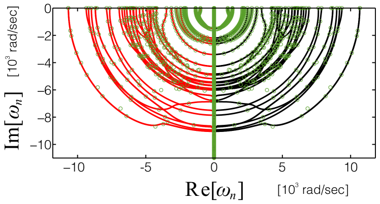
Figure 3 shows a comparison of both methods to calculate the normal modes as a function of for a system of 14 particles. The system is small enough that we can plot the trajectories of all the 84 normal modes. We see that for this system, equation 26 gives the same result as the direct calculation of normal modes via eigenvectors of the dynamical matrix (equation 13). We conclude that the alternative method of Meirovitch (1987), equation 26, works well and then we proceed to use it for large system sizes.
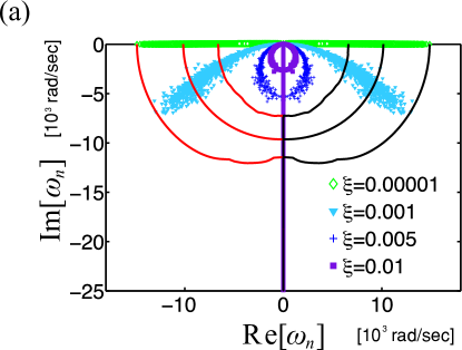
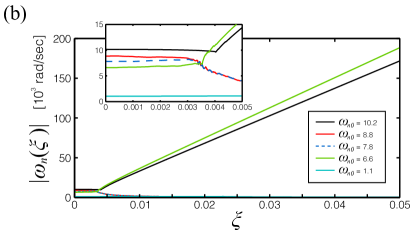
Figure 4a shows the results of the trajectories of the normal modes as a function of for a system of particles. The normal modes are calculated via equation 26. We start with a specific undamped mode and then follow its trajectory as a function of in the Re Im-plane. We follow the trajectories of specific undamped modes by increasing the damping parameter in small steps and using the method explained above. Since the system is large, we do not trace the trajectories of all 2400 modes. To indicate the general shape of the mode trajectories we trace that for three modes characterized by undamped frequencies and 15 rad/sec, as indicated by the solid red and black lines in the figure, respectively. In addition, we also plot all the modes for four values of as indicated in the figure.
In general, the theoretical predictions equations 18, 20 and 22 are in rather good agreement with the results in Figure 4; the small deviations can be traced back to the approximation equation 15 which is not exact in the considered packings. This plot shows that the modes follow a nearly circular trajectory as we change (the Menorah-shape traced in continuous black and red lines) as predicted by equation 17. When the modes lie on the imaginary axis in agreement with the prediction of equation 18. A cross-plot of Re[] vs. Im[], for fixed nearly follows equation 20, for modes which are not overdamped. The latter prediction is valid for small (light blue curve, ). For greater we find the circular plots predicted by equation 20 (see blue and purple curves for 0.4 and 0.8, respectively). The centers of the circles lie on the imaginary axis and they are characterized by a radius . The strong implication, then, is that all the normal mode frequencies for real granular media lie on or near a circle of radius centered on the point . (In our work, here, .)
To further test the prediction of circular trajectories, we plot the evolution of the absolute value of selected modes for increasing values of (Figure 4b). We find that the absolute value of the mode is nearly constant, corresponding to the circular trajectory, equation 19 for , until the critical value of damping unique to the individual modes. When approaches , the absolute value of the normal mode frequency is no longer constant and the mode becomes overdamped, with the result that either increases or decreases along the imaginary axis as a function of .
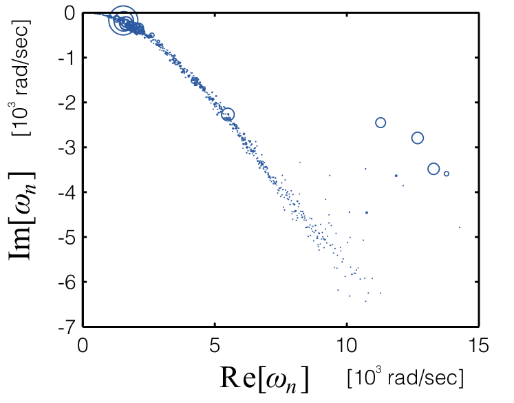
Figure 5 shows the normal modes for a system with a fixed value of . In this case, the relative residue of each mode is indicated by the size of the data point. The residue is indicative of the contribution of the mode to the effective mass (Valenza and Johnson, 2012; Hu et al., 2014); large residues correspond to modes with large contributions to the effective mass. The modes exhibit a parabolic dependence on consistent with equation 22, which is valid for this system characterized by small . However, we also observe that several modes with large residue do not lie on the parabola. As previously noted, the large residue indicates that these outliers make an important contribution to the effective mass. They are a direct manifestation of the breakdown of the approximation equation 15.
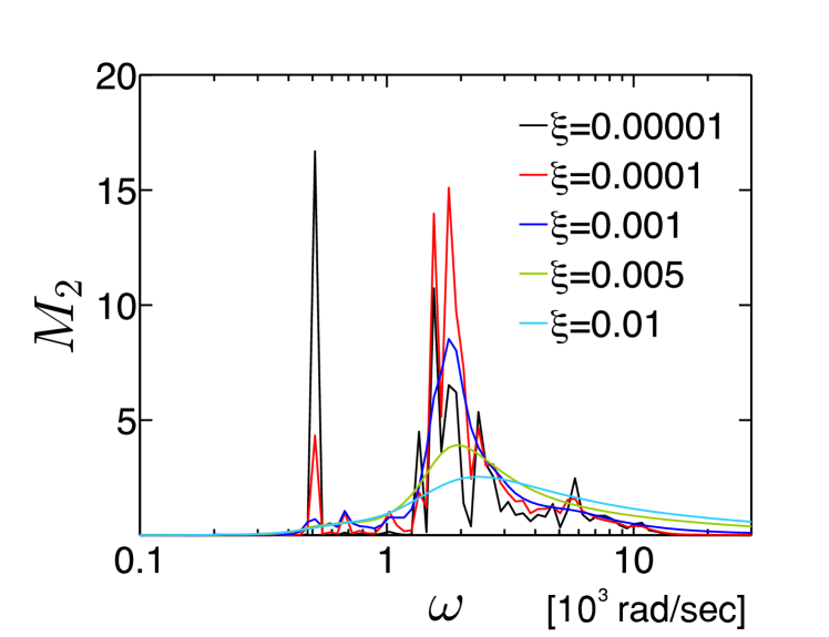
Figure 6 shows the imaginary part of the effective mass, , calculated via DEM, for different values of the damping parameter . As increases the large amplitude modes spread out over a larger frequency band, and modes characterized by a small amplitude, effectively disappear. That is, for small we find a large number of peaks in the effective mass. As increases, more and more peaks disappear. We also find a special low frequency mode less than 1000 rad/sec with a very large resonance peak indicating that this frequency contributes a lot to the attenuation of the medium. When the damping is increased from to , the peak almost disappears. Thus, even at small modes that make important contributions to dissipation can be overdamped. The strong attenuation of the first (low-frequency) peak is observed when increasing the damping parameter, compared to the high-frequency peaks. This effect is a consequence of equation 18, which states that the critical damping is inverse proportional to the frequency of the undamped mode.
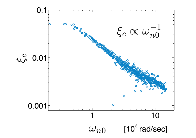
Finally, we test the scaling of the critical damping as a function of the frequency of the undamped mode , as suggested by equation 18. Figure 7 shows good agreement between the numerical estimation of and , confirming the inverse scaling law of equation 18. The deviations in the curve in Fig. 7 from equation 18 are explained due to the approximation of equation 15. This scaling law indicates that lower frequency modes are more resistant to becoming overdamped. Again, some high frequency modes do not obey the scaling behavior equation 18. These modes have a small value and therefore can be easily dampened.
CONCLUSIONS
In summary, we have explored the effects of interparticle damping on the normal modes in a granular medium. We find good agreement between the DEM simulations and the analytical predictions. As the interparticle damping is varied, the normal mode trajectories in the complex plane are nearly circular and the critical value of the damping parameter, , scales approximately as . For a fixed value of the damping parameter, , the normal mode frequencies lie nearly on the circle given by equation 20. These properties indicate that the assumption of proportionality, equation 15, is approximately valid, even though it is not strictly true. The strong implication is that these simulation results of ours have approximate validity to understanding dissipation effects in real granular systems. Specifically, the indication is that the normal mode frequencies of real granular systems lie on or near a circle of radius centered on the point , where is inversely proportional to the intergranular damping parameter.
A surprising observation is that there are some very special normal modes that do not obey this scaling law. The corresponding frequencies are easy to identify in trajectory plots and are characterized by a small critical damping parameter. These outliers can make large contributions to dissipation of acoustic energy in the granular medium. Overall, the theoretical approach allows for a systematic investigation of the normal mode frequencies not only for spherical particles, as presented here, but also for non-spherical particles as well to understand acoustics and dissipation in all granular media.
ACKNOWLEDGMENTS
We acknowledge financial support from DOE Office of Basic Energy Sciences, Chemical Sciences, Geosciences, and Biosciences Division, Grant DE-FG02-03ER15458, and NSF-CMMT. We thank F. Santibáñez and S. Reis for discussions and help with the manuscript.
REFERENCES
Alexander, S., 1998, Amorphous solids: their structure, lattice dynamics and elasticity: Phys. Rep. 296, 65-236.
Behringer, R. P. and J. T. Jenkins, 1997, Powders & Grains, Balkema.
Bhaskar, A. 1997, Criticality of damping in multi-degree-of-freedom systems: J. Appl. Mech. 64, 387–393.
Baule, A., R. Mari, L. Bo. L. Portal, H. A. Makse, 2013, Mean-field theory for random close packings of axisymmetric particles: Nature Commun. 4, 2194.
Baule, A. and H. A. Makse, 2014, Fundamental challenges in packing problems: from spherical to non-spherical particles: Soft Matter 10, 4423.
Brujić, J., P. Wang, C. Song, D. L. Johnson, O. Sindt, and H. A. Makse,, 2005, Granular dynamics in compaction and stress relaxation: Phys. Rev. Lett. 95, 128001.
Brujić, J., C. Song, P. Wang, C. Briscoe, G. Marty, and H. A. Makse, 2007, Fluorescent contacts measure the coordination number and entropy of a 3D jammed emulsion packing: Phys. Rev. Lett. 98, 248001.
Brunet, Th., X. Jia, and P. Mills, 2008, Mechanisms for acoustic absorption in dry and weakly wet granular media: Phys. Rev. Lett. 101, 138001.
Caughey, T. K., 1960, Classical normal modes in damped linear dynamic systems: J. Appl. Mech. 27, 269-271; Caughey, T. K. and M. E. J. O’Kelly, 1965, Classical normal modes in damped linear dynamic systems: J. Appl. Mech. 32, 583-588
Chen, Y.-C., I. Ishibashi, and J. T. Jenkins, 1988, Dynamic shear modulus and fabric: part I, depositional and induced anisotropy: Géotechnique 38, 25-32.
Cundall, P. A. and O. D. L. Strack, 1979, A Discrete Numerical Model for Granular Assemblies: Géotechnique 29, 47-65.
de Gennes, P.-G., 1996, Static compression of a granular medium: The “Soft Shell” model: Europhys. Lett. 35, 145-149.
Digby, P. J., 1981, The effective elastic moduli of porous granular rocks: J. Appl. Mech. 48, 803-808.
Domenico, S. N., 1977, Elastic properties of unconsolidated porous sand reservoirs: Geophysics 42, 1339-1368.
Garvey, S. D., J. E. T. Penny, and M. I. Friswell, 1998, The relationship between the real and the imaginary parts of complex modes: J. Sound & Vib. 212, 75-83.
Goddard, J. D., 1990, Nonlinear Elasticity and Pressure-dependent Wave Speeds in Granular Materials: Proc. R. Soc. Lond. A 430, 105-131.
Guyer, R. A. and P. A. Johnson, 1999, Nonlinear mesoscopic elasticity: Evidence for a new class of materials: Phys. Today 52, 30.
Henann, D. L., J. J. Valenza, D. L. Johnson, and K. Kamrin, 2013, Small amplitude acoustics in bulk granular media: Phys. Rev. E 88 042205.
Hsu, C-J., D. L. Johnson, R. A. Ingale, J. J. Valenza, N. Gland, and H. A. Makse, 2009, Dynamic effective mass of granular media: Phys. Rev. Lett. 102, 058001.
Hu, Y., D. L. Johnson, J. J. Valenza, F. Santibáñez, and H. A. Makse, 2014, Stress-dependent normal mode frequencies from the effective mass of granular matter: Phys. Rev. E 89, 062202.
Inman, D. J. and A. N. Andry, 1980, Some results on the nature of eigenvalues of discrete damped systems: J. Appl. Mech. 47, 927–930.
Jin, Y. and H. A. Makse, 2010, A first-order phase transition defines the random close packing of hard spheres: Physica A 389, 5362-5379 (2010).
Johnson, D. L., L. Schwartz, D. Elata, J. G. Berryman, B. Hornby, A. N. Norris, 1998, Linear and nonlinear elasticity of granular media: Stress-Induced anisotropy of a random sphere pack: ASME J. Appl. Mech. 65, 380-388.
Johnson, K. L., 1985, Contact Mechanics: Cambridge University Press.
Johnson, P. A., B. Zinszner, and P. N. J. Rasolofosaon, 1996, Resonance and nonlinear elastic phenomena in rock: J. Geophys. Res. 101, 11553-11564.
Landau, L. D. and E. M. Lifshitz, 1970, Theory of Elasticity: Pergamon.
Lehoucq, R. B. and D. C. Sorensen, 1996, Deflation techniques for an implicitly re-started Arnoldi iteration: SIAM J. Matrix Analysis and Applications 17, 789-821.
Magnanimo, V., L. La Ragione, J. T. Jenkins, P. Wang, and H. A. Makse, 2008, Characterizing the shear and bulk moduli of an idealized granular material: Europhys. Lett. 81, 34006.
Makse, H. A., N. Gland, D. L. Johnson, and L.M. Schwartz, 1999, Why effective medium fails in granular materials: Phys. Rev. Lett. 83, 5070-5073.
Makse, H. A., D. L. Johnson, and L. M. Schwartz, 2000, Packing of compressible granular materials: Phys. Rev. Lett. 84, 4160-4163.
Makse, H. A., J. Brujić, and S. F. Edwards, 2004, Statistical mechanics of jammed matter: in The Physics of Granular Media, H. Hinrichsen and D. E. Wolf (eds.) Wiley.
Meirovitch, L. , 1987, Principles and techniques of vibrations: Prentice-Hall.
Norris, A. N. and D. L. Johnson, 1997, Nonlinear elasticity of granular media: J. Appl. Mech. 64, 39-49.
O’Connell, R. J., and B. Budiansky, 1977, Viscoelastic properties of fluid-saturated cracked solids: J. Geophys. Res. B 82, 5719-5735.
O’Hern, C. S., L. E. Silbert, A. J. Liu, and S. R. Nagel, 2003, Jamming at zero temperature and zero applied stress: The epitome of disorder: Phys. Rev. E 68, 011306.
Shafer J., S. Dippel,and D. E. Wolf, 1996, Force schemes in simulations of granular materials: J. Phys. I (France) 6, 5-20.
Silbert, L. E., A. J. Liu, and S. R. Nagel, 2005, Vibrations and diverging length scales near the unjamming transition: Phys. Rev. Lett. 95, 098301.
Somfai, E., et al., 2007, Critical and noncritical jamming of frictional grains: Phys. Rev. E 75, 020301R.
Song, C., P. Wang, and H. A. Makse, 2008, Phase diagram for jammed matter: Nature 453, 629-632.
Sorensen, D. C., 1992, Implicit Application of polynomial filters in a k-step Arnoldi method: SIAM J. Matrix Analysis and Applications, 13, 357-385.
Sun, J. C., H. B. Sun, L. C. Chow, and E. J. Richards, 1986, Predictions of total loss factors of structures, part II: Loss factors of sand-filled structure: J. Sound and Vib. 104, 243-257.
Valenza, J. J., C.-J. Hsu, R. Ingale, N. Gland, H. A. Makse, and D. L. Johnson, 2009, Dynamic effective mass of granular media and the attenuation of structure-borne sound: Phys. Rev. E 80, 051304.
Valenza, J. J. and D. L. Johnson, 2012, Normal-mode spectrum of finite-sized granular systems: The effects of fluid viscosity at the grain contacts: Phys. Rev. E 85, 041302.
Walton, K., 1987, The effective elastic moduli of a random packing of spheres: J. Mech. Phys. Solids 35, 213-226.
Winkler, K. W., 1983, Contact stiffness in granular porous materials: Comparison between theory and experiments: Geophys. Res. Lett. 10, 1073-1076.
Wyart, M., S. R. Nagel, and T. A. Witten, 2005a, Geometric origin of excess low-frequency vibrational modes in weakly connected amorphous solids: Europhys. Lett. 72, 486-492.
Wyart, M., L. E. Silbert, S. R. Nagel S. R. and T. A. Witten, 2005b, Effects of compression on the vibrational modes of marginally jammed solids: Phys. Rev. E 72, 051306.
FIG. 1. Schematic view of the simulation box and particles. The simulations consider periodic boundary conditions. The walls are made of fixed particles of the same features of the particles in the bulk. The figure shows a system prepared after the relaxation under gravity has finished. The walls are shaken during the dynamical calculation of the effective mass with an acceleration and the force is measured at the bottom of the cup to obtain the effective mass via equation 1.
FIG. 2.Comparison of theoretical estimation of the effective mass via equation 12 and the direct dynamical measurements using the numerically generated packings with DEM by shaking the packing at a given frequency . DEM results are shown by the symbols for two damping parameters ms and ms and separately for the real and imaginary part of the effective mass , as indicated. The DEM shaking simulation results are obtained from the frequency sweep with amplitude m. The theory lines correspond to the solution of the right hand side of equation 12: , where is calculated as discussed in the text. The two different methods of computation are in good agreement with each other.
FIG. 3. Trajectories of all the 84 resonance frequencies for a small packing of 14 particles. This plot shows the comparison between the trajectories of calculated by the Meirovitch method of equation 25 (circles) with the direct determination of the determinant of the dynamical matrix (line trajectories). We confirm that both methods gives the same result for the normal frequencies. This result indicates that equation 25 is an efficient way to calculate the normal modes, and it is used then in the calculations for larger system sizes in the rest of the paper. The trajectories follow the Menorah-like shapes which are further investigated in Fig. 4 for a larger system.
FIG. 4. (a) Locus of all the complex-valued normal mode frequencies of our large system for four different values of the damping parameter, . The normal modes are calculated via the solution of equation 25. Also shown are the trajectories of three of the normal mode frequencies as is varied from low to high values. The frequencies approximately follow equations 19 and 20. The stated values for are in millisec. (b) vs. shown for a few selected modes obtained from (a) which shows how nearly circular the trajectories are up to the point of critical damping.
FIG. 5. Distribution of normal mode frequencies in the complex plane for a given fixed small damping ms for . The size of the symbol is proportional to the resonance mode residue.
FIG. 6. Imaginary effective mass calculated via the direct dynamical shaking of the medium for increasing values of , in millisec, for .
FIG. 7. Critical damping as function of the normal mode frequency of the undamped mode for . The theoretical prediction in equation 18 is in satisfactory statistical agreement with the numerical results.