Stress-dependent normal mode frequencies from the effective mass of granular matter

Abstract

A zero-temperature critical point has been invoked to control the anomalous behavior of granular matter as it approaches jamming or mechanical arrest. Criticality manifests itself in an anomalous spectrum of low-frequency normal modes and scaling behavior near the jamming transition. The critical point may explain the peculiar mechanical properties of dissimilar systems such as glasses and granular materials. Here, we study the critical scenario via an experimental measurement of the normal modes frequencies of granular matter under stress from a pole decomposition analysis of the effective mass. We extract a complex-valued characteristic frequency which displays scaling $|\omega^{*}(\sigma)|\sim\sigma^{\Omega^{\prime}}$ with vanishing stress $\sigma$ for a variety of granular systems. The critical exponent is smaller than that predicted by mean-field theory opening new challenges to explain the exponent for frictional and dissipative granular matter. Our results shed light on the anomalous behavior of stress-dependent acoustics and attenuation in granular materials near the jamming transition.

I Introduction

In granular media, a jammed system results if the particles pack together at high enough density such that all the particles are touching their neighbors jamming . As a result, the material undergoes a jamming transition above which the system remains arrested in a jammed state and is able to withstand a sufficiently small applied stress. The jamming transition occurs at a particularly subtle point where the particles have no redundant mechanical constraints, i.e. they are isostatic alexander ; moukarzel ; makse ; ohern1 . The system is a fragile solid that is highly susceptible to external perturbations. For instance, cutting a set of particle contacts creates floppy modes which necessitate global rearrangement to rebalance the system alexander ; moukarzel ; Matthieu2005 ; Wyart2005 ; liu-review .

This critical point has important consequences for the mechanical properties of granular matter. In particular, there exists an excess of low-frequency modes above that expected from the Debye scaling of phonons in elastic solids ohern ; silbert2005 . When the system is jammed, a band of excess modes exists for $\omega>\omega_{D}^{*}$, $\omega_{D}^{*}$ is a characteristic frequency that vanishes as the jamming transition is approached silbert2005 [the subscript indicates that this frequency determines the limit of validity of Debye scaling in the density of states]. For $\omega<\omega_{D}^{*}$ one has the usual Debye density of states. The system is argued to be critical with a diverging correlation length $\ell^{*}$ Wyart2005 scaling as the inverse of the characteristic frequency. The excess modes distinguish an isostatic critical state at scales below $\ell^{*}$ from an elastic solid at scales larger than $\ell^{*}$ Matthieu2005 ; Wyart2005 . The characteristic frequency follows scaling law ohern ; silbert2005 ; liu-review ; Matthieu2005 ; Wyart2005 ; friction1 ; xu :

$$\omega_{D}^{*}\sim(\phi-\phi_{c})^{\Omega}\sim\sigma^{\Omega^{\prime}},$$ (1)

with external stress, $\sigma$, or volume fraction, $\phi$, measured with respect to the jamming point $\Delta\phi=\phi-\phi_{c}$ (eg random close packing or point J ohern ; makse ; ohern1 ).

The static properties of jammed systems are also characterized by scaling laws. In particular, the average coordination number scales as

$$Z-Z_{c}\sim(\phi-\phi_{c})^{1/2},$$ (2)

with scaling exponent approximately independent of friction makse ; ohern1 ; ohern ; liu-review ; friction1 ; zhang ; Matthieu2005 . Here, $\Delta Z=Z-Z_{c}$ measures the excess contacts from the minimal isostatic coordination number for frictionless grains $Z_{c}=6$, or a critical value $4\leq Z_{c}\leq 6$ for frictional grains in 3D friction1 ; zhang ; brujic-prl . The constitutive law between stress and volume fraction is

$$\sigma\sim(\phi-\phi_{c})^{\alpha},$$ (3)

where $\alpha=3/2$ for Hertzian spheres and $\alpha=1$ for linear springs. Thus, $\Omega=\Omega^{\prime}\alpha$.

To compare across systems with different constitutive laws, we separate the trivial stress dependence of $\alpha$ from the non-trivial structural dependence characterized by exponent $\delta$:

$$\omega_{D}^{*}\sim\Delta\phi^{(\alpha-1)/2}\Delta\phi^{\delta},$$ (4)

with $\delta=\Omega+(1-\alpha)/2$. Theory Wyart2005 ; Matthieu2005 has found using a variational argument of boundary contact removal process for a system of particles with linear constitutive law ($\alpha=1)$

$$\omega_{D}^{*}(\Delta Z)\sim\Delta Z,\,\,\,\,\,\,\mbox{($\alpha=1$, mean-field scaling)},$$ (5)

yielding a prediction $\delta_{\rm th}=1/2$, using Eq. (2), which agrees with simulations of frictionless particles silbert2005 .

So far, the scaling behavior of Eq. (1) has not been tested by direct experimental measurements on zero-temperature granular matter. Indeed, experiments cannot calculate the density of states by directly measuring the interparticle potential as done in simulations ohern ; silbert2005 . Here, we employ a novel dynamical measurement to measure the normal modes.

Previous experiments focused on thermally agitated colloidal glasses and supercooled liquid systems kurchan ; Chen2010 ; Widmer2008 . In contrast, granular materials are athermal (the energy necessary to displace a grain is much larger than the thermal energy $\sim 10^{14}$ times) and friction dominated. Moreover, Eq. (1) was derived for non-frictional non-dissipative systems Matthieu2005 ; Wyart2005 . In the case of real granular media, dissipation plays a key role in governing the dynamics JValenza2012 . In this work, we develop an experimental study of the stress-dependent normal modes frequencies for the case of granular matter. We demonstrate that the normal mode spectrum of a finite sized granular system can be determined through a pole decomposition of the frequency-dependent effective mass Chaur2009 ; JValenza2009 ; JValenza2012 . The results of this analysis supports the scaling hypothesis Eq. (1) in a realistic athermal and dissipative medium. However, the exponents characterizing this granular medium are smaller than those predicted by theory Eq. (5) Wyart2005 ; Matthieu2005 .

II Experiments

We employ a dynamical effective mass measurement to obtain the normal modes which complements other measures of the normal modes obtained from the Fourier transform of the velocity autocorrelation function and the eigenvalues of the displacement correlation matrix ohern ; silbert2005 ; xu ; friction1 ; liu-review . Specifically, we measure the frequency dependent effective mass, $\tilde{M}(\omega)$, introduced previously in Chaur2009 ; JValenza2009 ; JValenza2012 , of a granular medium held in a cup under varying stress.

The full experimental program has been developed in Chaur2009 ; JValenza2009 ; JValenza2012 and it is described in detail in Appendix X. Here we refer to the most important aspects of the experiments and the corresponding set of predictions. The stress-dependent scaling behavior of the normal mode spectrum of the granular system can be determined through a pole decomposition of the frequency-dependent effective mass Chaur2009 ; JValenza2009 ; JValenza2012 . We use a variety of granular systems consisting of particles of different sizes (ranging from $\sim$150 microns to millimeters), different shapes (irregular and spherical), different materials (tungsten, steel and glass), and different damping conditions (particles coated with silicone oil and uncoated).

An important factor in the dynamics of this system is the existence of dissipative modes. Accordingly, our initial experiments follow the procedure described in reference JValenza2012 to lightly coat the tungsten particles (nominal size $\sim$150 $\mu$m) with silicone oil (PDMS), which yields a system with known dissipative properties— later, we will show results for uncoated particles. The weakly wet powder is poured into a cup, and the cup is tapped to encourage the powder to settle and yield a flat free surface, Fig. 1. Finally, a standard mechanical compaction protocol is followed brujic ; edwards ; briscoe ; Baule to prepare the system in a reversible state which yields a reproducible $\tilde{M}(\omega)$.

Once loaded, the cup is subjected to a vertical sinusoidal vibration at angular frequency $\omega$. The force, $\tilde{F}(\omega)$, is measured by a force gauge mounted between the cup and the shaker, and the acceleration, $\tilde{a}(\omega)$, is taken as the average of that measured at two points on the opposite end of a single diameter. The effective mass of the granular medium is the causal response function Chaur2009 ; JValenza2009 ; JValenza2012 :

$$\tilde{M}(\omega)=\frac{\tilde{F}(\omega)}{\tilde{a}(\omega)}-M_{c},$$ (6)

where $M_{c}$ is the mass of the empty cup. Here, $\tilde{M}(\omega)=M_{1}(\omega)\>+\>iM_{2}(\omega)$ is complex-valued and reflects the partially in-phase and out-of-phase motion of the individual grains relative to the cup motion. $M_{1}$ is indicative of the elastic, and $M_{2}$ of the dissipative characteristics of the powder. Figures 2a and b show $M_{1}(\omega)$ and $M_{2}(\omega)$ for tungsten systems exposed to an incrementally increasing uniaxial confining stress, $\sigma$. In all cases, the lowest characteristic frequency mode manifests itself as the sharpest resonance peak in $M_{2}(\omega)$. This peak and the other, lower amplitude, modes in the system are characterized by a complex-valued normal mode frequency, $\omega_{n}$. Roughly speaking, Re$[\omega_{n}]$ is given by the position of the frequency mode, and Im$[\omega_{n}]$ is half of the full width at half max of the frequency mode.

To accurately infer $\omega_{n}$ from the data in Fig. 2 we analyze $\tilde{M}(\omega)$ within the context of a theory of damped and frictional contact forces JValenza2012 , which generalizes the results of previous analyses Matthieu2005 ; Wyart2005 . While previous theories have considered central force systems Matthieu2005 ; Wyart2005 , interpreting the dynamic response of our experiments necessitates a formalism that accounts for translational and rotational degree of freedom and damped modes. We develop such a formalism next.

III Theory

III.1 Interparticle force-law

In general the granular medium is modeled as a set of grains held in a rigid cup. The theory is valid for any linearized set of contact forces. Without loss of generality, below we define it for the specific case of Hertz-Mindlin contact forces. The normal force between any two contacting particles with radius $R$ is brilliantov ; wolf :

$$F_{n}=\frac{2}{3}k_{n}R^{1/2}x_{ij}^{3/2},$$ (7)

where the normal deformation (1/2 the overlap between the spheres) between the neighboring grains is $x_{ij}=\frac{1}{2}[2R-|\mathbf{x}_{i}-\mathbf{x}_{j}|]$, $\mathbf{x}_{i,j}$ are the position vectors, and $k_{n}$ is the normal spring constant. The latter is defined in terms of the corresponding material properties. The normal elastic constant is

$$k_{n}=4G_{g}/(1-\nu_{g}),$$ (8)

where $G_{g}$ is the shear modulus, and $\nu_{g}$ is the Poisson’s ratio of the material from which the grains are made.

The tangential force between neighboring grains in contact is wolf :

$$\Delta F_{t}=k_{t}(Rx_{ij})^{1/2}\Delta s,$$ (9)

where

$$k_{t}=8G_{g}/(2-\nu_{g}),$$ (10)

is the tangential spring constant, and the variable $s$ is defined such that the relative shear displacement between the two grain centers is $2s$. Finally, Coulomb friction with interparticle friction coefficient $\mu$ imposes $F_{t}\leq\mu F_{n}$ at every contact.

From the definition of particle interactions, the elastic spring constant tensor is written in terms of the normal ($N$) and transverse ($T$) stiffnesses as:

$$\mathbf{K}_{ij}=k^{N}(x_{ij})\mathbf{\hat{d}}_{ij}\mathbf{\hat{d}}_{ij}+k^{T}(x_{ij})[\mathbf{I}-\mathbf{\hat{d}}_{ij}\mathbf{\hat{d}}_{ij}],$$ (11)

where $\mathbf{\hat{d}}_{ij}$ denotes the direction of the normal displacement and we use the dyadic notation. Since we are interested in infinitesimal displacements, without loss of generality we use a linearized version of the Hertz-Mindlin force law Eqs. (7) and (9) and define the elastic stiffnesses as:

$$k^{N}(x_{ij})=k_{n}R^{1/2}x_{ij}^{1/2},$$ (12)

and

$$k^{T}(x_{ij})=k_{t}R^{1/2}x_{ij}^{1/2},$$ (13)

where $k_{n}$ is the normal spring constant defined in terms of the corresponding material properties above. That is, we use the Hertz-Mindlin force law linearized about the static value of the normal compression of contacts. The resulting elastic stiffness is simply the slope evaluated at $x_{ij}$. The tangential force between neighboring grains in contact is defined in terms of the tangential spring constant $k_{t}$ above.

The dissipative properties of the particles are defined as follows. The definition of the damping tensor $\mathbf{B}_{ij}$ involves a normal damping and a tangential damping in analogy to the definition of the elastic matrix Eq. (11). A representation of the damping matrix in terms of the first order Taylor expansion gives the following form which is an extension of the original Hertz approach assuming the material to be viscoelastic instead of elastic. The form of the damping tensor $\mathbf{B}_{ij}$ has been calculated by Kuwabara and Kono kono and Brilliantov et al. brilliantov (see also wolf for a review):

$$\mathbf{B}_{ij}=\gamma^{N}(x_{ij})\mathbf{\hat{d}}_{ij}\mathbf{\hat{d}}_{ij}+\gamma^{T}(x_{ij})[\mathbf{I}-\mathbf{\hat{d}}_{ij}\mathbf{\hat{d}}_{ij}].$$ (14)

If the particles, $i$ and $j$, are not in contact ($|\mathbf{x}_{j}-\mathbf{x}_{i}|>2R$), we set both $\mathbf{K}_{ij}=0$ $\mathbf{B}_{ij}=0$.

Both damping constants, normal $\gamma^{N}(x_{ij})$ and tangential $\gamma^{T}(x_{ij})$, are proportional to the respective elastic constants in the elastic counterparts $k^{N}(x_{ij})$ and $k^{T}(x_{ij})$. This is seen by following the calculations of Brilliantov brilliantov for the dissipative force between two contacting particles. The total force acting between viscoelastic particles can be derived from the total stress tensor taking into account the elastic and dissipative parts (see Landau for details landau ):

$$\hat{\sigma}=\hat{\sigma}_{(el)}+\hat{\sigma}_{(dis)}.$$ (15)

The calculations are simplified since the elastic and dissipative parts of the stress tensor are related in the quasi-static limit brilliantov ; landau :

$$\hat{\sigma}_{(dis)}=\dot{x}_{ij}\frac{\partial}{\partial x_{ij}}\hat{\sigma}_{(el)}.$$ (16)

This leads to a dissipative force of the form:

$$F^{N}_{dis}=\xi k_{n}R^{1/2}x_{ij}^{1/2}\dot{x}_{ij},$$ (17)

where $\xi$ is the damping parameter with unit of time and related to the elastic and viscoelastic constant of the material from which the particles are made. From landau we have:

$$\xi=\frac{1}{2}\frac{(3\eta_{2}-\eta_{1})^{2}}{(3\eta_{2}+2\eta_{1})}\Big{[}\frac{(1+\nu_{g})(1-2\nu_{g})}{2G_{g}}\Big{]},$$ (18)

where $\eta_{1}$ and $\eta_{2}$ are the viscous constants of the material of the particles (see Eq. (23) in brilliantov ). Comparing with the Hertzian counterpart Eq. (7) we have the formal relation for the total force in the normal direction:

$$F^{N}_{tot}=const\Big{(}x_{ij}^{3/2}+\xi x_{ij}^{1/2}\dot{x}_{ij}\Big{)}.$$ (19)

A similar derivation holds for the tangential components, for which we have brilliantov :

$$F^{T}_{dis}=\xi k_{t}R^{1/2}x_{ij}^{1/2}\dot{s}.$$ (20)

These considerations leads to Eq. (14) with

$$\gamma^{N}(x_{ij})=\xi k^{N}(x_{ij}),$$ (21)

and

$$\gamma^{T}(x_{ij})=\xi k^{T}(x_{ij}).$$ (22)

Combining these equations we arrive at:

$$\mathbf{B}_{ij}=\xi\mathbf{K}_{ij},$$ (23)

which is used later to understand the trajectories of the normal mode frequencies in the complex plane, considered as functions of $\xi$: $\omega_{n}=\omega_{n}(\xi)$.

The constitutive contact laws expressed by the Hertz-Mindlin theory imply the trivial scaling between the stress and strain (or volume fraction) under compression HMakse :

$$\sigma\sim\epsilon^{\alpha},$$ (24)

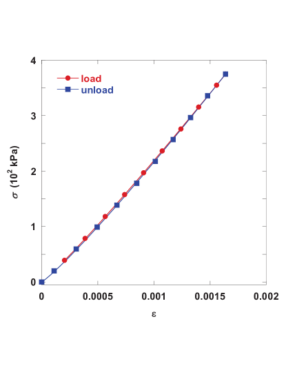
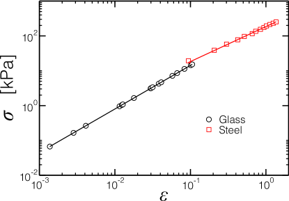
(a) (b)

Figure 3: (Color online) Force constitutive law. We measure the axial stress vs. strain response of (a) the tungsten powder confined in the cup and find an approximate power-law with exponent $1.15\pm 0.01$, averaged over load and unload, (b) the packing of glass beads and steel balls with exponents $\alpha$ given in Table 1.

with $\alpha=3/2$ for Hertz contact force law, Eq. (7), $\sigma$ is the uniaxial stress and $\epsilon$ is the strain. When the constitutive particles follow other force law, the exponent $\alpha$ is modified accordingly. In fact, $\alpha=3/2$ is expected for a collection of monodisperse spherical Hertzian grains, which is not an accurate description for the system we study here. Therefore, we use a mechanical testing machine to measure the stress-strain relationship exhibited by the tungsten powder and the system of glass and steel beads confined in the cup. To perform this characterization, we sit a solid stainless steel plunger on top of the powder. As demonstrated in Fig. 3a, we find a weakly non-linear stress-strain response of the tungsten powder. For the powder we use in this study, the power law exponent always falls significantly below that predicted by Eq. (24), $\alpha=1.15\pm 0.01$. We also test the constitutive laws for the systems of glass beads and steel beads (Fig. 3b) obtaining the $\alpha$ exponent summarized in Table 1.

III.2 Theory of normal modes in a dissipative medium

In what follows, $\mathbf{x}_{i}$, and $\mathbf{u}_{i}$ denote the equilibrium position, and displacement from equilibrium, respectively, of the $i$-th particle. The variables $\theta_{i}$ represent the librational angles of the i-th particle. In addition, $\mathbf{W}=W\mathbf{\hat{z}}$ represents the displacement of the cup wall in the $z$-direction. In the associated experiment, $\mathbf{W}=W\mathbf{\hat{z}}$ is 1 micron, at least three orders of magnitude smaller than $R$, therefore, all $\mathbf{u}_{i}$ are infinitesimal and the linear equation of motion for the $i$-th particle with mass $m$ is:

$$-m\omega^{2}\mathbf{u}_{i}=\mathbf{K^{\prime}}_{i\omega}[\mathbf{u}_{i}+\theta_{i}\times\mathbf{\hat{d}}_{iw}-\mathbf{W}]+\\ \sum_{j}\mathbf{K^{\prime}}_{ij}[\mathbf{u}_{j}-\mathbf{u}_{i}+\theta_{j}\times\mathbf{\hat{d}}_{ji}-\theta_{i}\times\mathbf{\hat{d}}_{ij}],$$ (25)

where, $\mathbf{d}_{ij}=(1/2)(\mathbf{x}_{i}-\mathbf{x}_{j})$ for the case when neighboring particles are identical spheres, and the subscript, $w$ indicates a particle interacting with the cup wall. The equations of motion for the angular variables are:

$$-\omega^{2}\mathbf{I}_{i}\dot{\theta}_{i}=-\mathbf{d}_{iw}\times\mathbf{K^{\prime}}_{i\omega}[\mathbf{u}_{i}+\theta_{i}\times\mathbf{\hat{d}}_{iw}-\mathbf{W}]+\\ \sum_{j}\mathbf{d}_{ij}\times\mathbf{K^{\prime}}_{ij}[\mathbf{u}_{j}-\mathbf{u}_{i}+\theta_{j}\times\mathbf{\hat{d}}_{ji}-\theta_{i}\times\mathbf{\hat{d}}_{ij}].$$ (26)

The stiffness matrix $\mathbf{K^{\prime}}_{ij}$ modulates the elastic and viscous interactions between neighboring particles and is defined in terms of the elastic matrix $\mathbf{K}_{ij}$ and the damping matrix $\mathbf{B}_{ij}$ as defined above:

$$\mathbf{K^{\prime}}_{ij}=\mathbf{K}_{ij}-i\omega\mathbf{B}_{ij}.$$ (27)

Similarly, $\mathbf{K^{\prime}}_{iw}$ describes the elastic and viscous interaction between a particle and the wall of the cup; it is zero for particles not in contact with the wall. Next we write a compact form of these equations of motion, Eqs. (25) and (26).

The linearized equation of motion for the $i-$th particle in the system of $N$ particles with mass $m$ can be succinctly written as:

$$H_{ij}(\omega)u_{j}=K_{i\omega}W,\,\,\,\,\,\,\mbox{$i,j=1:6N$},$$ (28)

where the dynamical matrix is:

$$H_{ij}(\omega)=-m\delta_{ij}\omega^{2}-i\omega B_{ij}+K_{ij}.$$ (29)

Each term in $H_{ij}$ accounts for the inertial, dissipative and elastic interactions at the contact between particles $i$ and $j$, respectively. The vector $\{u_{j}\}$ represents the set of $3N$ particle displacements and $3N$ particle rotations, and $K_{i\omega}$ is the generalized spring constant connecting a particle to the walls of the cup which moves oscillatory in the $z$ direction with amplitude $W$. The effective mass is obtained by inverting the matrix $\mathbf{H}$ JValenza2012 :

$$\tilde{M}(\omega)=m[H^{-1}(\omega)]_{ij}K_{j\omega}.$$ (30)

This result formalizes the relation between the resonance peaks in the effective mass and the normal mode frequency spectrum. The peaks observed in $\tilde{M}(\omega)$ (Fig. 2) are due to the set of normal modes, $e_{j}^{n}$, that are a solution to Eq. (28) when there is no forcing by the cup, $W=0$, i.e.,

$$H_{ij}(\omega_{n})e_{j}^{n}=0.$$ (31)

The normal modes are those eigenvectors of $\mathbf{H}$ for which the corresponding eigenvalue is zero, and they occur at the complex-valued frequencies, $\omega_{n}$.

The normal mode frequencies, $\omega_{n}$, are the non-trivial solutions of Eq. (31), in which the eigenvalue is 0. Regardless the properties of the matrices $\mathbf{K,B}$ it is a rigorous result that for values of $\xi$ below a critical and finite value, $\xi_{m}$, all the modes are underdamped InmanAndry , meaning $\Re(\omega_{n})\neq 0\>\>\forall\;n\;$. Similarly, there is another finite, critical value, $\xi_{M}$, such that when $\xi\geq\xi_{M}$ all the modes are overdamped Bhaskar : $\Re(\omega_{n})\equiv 0\;\;\forall\;n$. As $\xi$ is increased from $\xi_{m}$ to $\xi_{M}$ each branch becomes critically damped at the values $\xi_{c}$ viz: $\omega_{n}(\xi_{c})=i\lambda_{n}\>\>\>n=1,2,...$. All normal modes have the same functional dependence on $\xi$ in the vicinity of such a critical point. Let $D(\lambda,\xi)=det\{H_{ij}(\omega=i\lambda,\xi)\}$. In the vicinity of the critical damping point $\lambda=\lambda_{nc},\;\xi=\xi_{nc}$ we may expand $D$ in a Taylors series:

$$\begin{array}[]{r}D(\lambda,\xi)=a_{n}(\lambda-\lambda_{nc})+b_{n}(\xi-\xi_{nc})+d_{n}(\lambda-\lambda_{nc})^{2}+\\ \\ e_{n}(\lambda-\lambda_{nc})(\xi-\xi_{nc})+f_{n}(\xi-\xi_{nc})^{2}\;+\;\ldots\end{array}\>\>\>,$$ (32)

where

$$\begin{array}[]{c}a_{n}=\frac{\partial D}{\partial\lambda}|_{(\lambda_{nc},\xi_{nc})}\>\>\>b_{n}=\frac{\partial D}{\partial\xi}\mid_{(\lambda_{nc},\xi_{nc})}\\ \\ d_{n}=(1/2)\frac{\partial^{2}D}{\partial\lambda^{2}}|_{(\lambda_{nc},\xi_{nc})}\>\>\>e_{n}=\frac{\partial^{2}D}{\partial\lambda\partial\xi}|_{(\lambda_{nc},\xi_{nc})}\\ \\ f_{n}=(1/2)\frac{\partial^{2}D}{\partial\xi^{2}}|_{(\lambda_{nc},\xi_{nc})}\end{array}$$ (33)

The coefficients $a_{n},b_{n},\ldots,f_{n}$ are all real-valued because $\{a_{i}^{j}\},\lambda_{nc}$ and $\xi_{nc}$ are all real-valued. $\lambda_{nc}$ is a double root of $D$ because it represents the coalescence of two distinct complex-conjugate roots in the limit $\xi\rightarrow\xi_{nc}^{-}$. Accordingly, $a_{n}\equiv 0$. One may solve for the roots of Eq. (32):

$$\omega_{n}=i\lambda_{n}=i\lambda_{nc}\pm ig_{n}(\xi-\xi_{nc})^{1/2}+\mathcal{O}(\xi-\xi_{nc})^{+1}\>\>\>,$$ (34)

where $g_{n}=\sqrt{-b_{n}/d_{n}}$ is real-valued because $\lambda_{n}$ is real-valued when $\xi>\xi_{nc}$.

Since $\mathbf{H}$ is a $6N\times 6N$ matrix, there are 12$N$ normal modes in this model. In practice, the effective mass can be understood in terms of a subset of these normal modes, which correspond to the modes located in the complex region of interest $[-\omega_{M}\leq{\rm Re}[\omega_{n}]\leq+\omega_{M}\;:\>\>-\omega_{M}\leq{\rm Im}[\omega_{n}],\leq 0]$, where $\omega_{M}$ is the maximal frequency measured in the experiment. The frequency dependence of $\tilde{M}(\omega)$ can be expressed in terms of this subset of normal modes through a pole decomposition JValenza2012 as described in the next section.

Thus, this set of equations allow for an experimental measurement of the normal mode frequencies directly from the effective mass.

IV Pole decomposition

The matrix $\mathbf{H}$ is complex-valued, frequency-dependent and symmetric. A non-Hermitian matrix like $\mathbf{H}$ may lack, in general, the property that its eigenvectors form a complete orthonormal basis 19 . However, according to a recent theorem by Tzeng and Wu 20 , there still exists $6N$ orthonormal vectors which satisfy the following modified eigenvector problem:

$$H_{ij}e_{j}^{n}=\lambda^{n}e_{i}^{n*},$$ (35)

where the eigenvalues $\lambda^{n}$ are complex valued and the asterisk denotes conjugation. A normal mode of the system is a solution to the set of Eqs. (25) and (26) in which there is no forcing by the cup: $W=0$. The corresponding displacements or rotations are the eigenvectors of $H$ whose eigenvalues are zero, i.e., $\lambda^{n}(\omega_{n})=0$. If we expand to first order: $\lambda^{n}(\omega)=\alpha^{n}(\omega-\omega_{n})+O(\omega-\omega_{n})^{2}$, and introduce this expansion into Eq. (30), we obtain the pole expansion:

$$\tilde{M}(\omega)=\sum_{n}\frac{A_{n}}{\omega-\omega_{n}},$$ (36)

with the residues given by

$$A_{n}=\frac{me^{n}_{i}(\omega_{n})e_{j}^{n}(\omega_{n})K_{jw}(\omega_{n})}{\alpha^{n}}.$$ (37)

In reference JValenza2012 it was demonstrated that the sum Eq. (36), is an exact expression for the effective mass. This allows us to use the rational function approximation, $\tilde{M}_{RF}$ discussed in the following section to extract the normal mode frequencies from the effective mass. The matrix $\mathbf{A_{n}}$ are the residues of the poles representing the strength of each resonance $\omega_{n}$. Using this expansion, which can be proved to be exact JValenza2012 , the set of normal modes and residues $\{\omega_{m},A_{m}\}$ can be determined from the experimental data of Fig. 2 via a search of all zeros of the rational function $M^{-1}$ analytically continued to the complex plane. We describe this procedure in the next Section V.

V Rational function decomposition to extract normal modes

We use the measured effective mass to extract the normal modes via the pole decomposition described by Eq. (36). Here, we describe the numerical procedure for generating the rational function interpolation of our data $\tilde{M}_{RF}$, which we use to determine the poles and the residues in our system.

In the experiments, we measure the effective mass $\tilde{M}(\omega_{i}^{e})$ at a series of discrete frequencies $e=1:1490$ from 100 Hz to a maximum frequency of 15 kHz. Using the reflection property, $\tilde{M}(-\omega_{i}^{e*})=\tilde{M}^{*}(\omega_{i}^{e})$, we extend the experimental data to negative real-valued frequencies, and we set $\tilde{M}(0)=M_{0}$, the static mass of the powder. So we are working with 2981 data points on the real frequency axis.

To search for the normal mode frequencies we require a complex valued function that passes through all the data points on the real axis. To this end we employ the Bulirsch-Stoer algorithm Bulirsch-Stoer-algorithm to determine a rational interpolation $R_{i(i+1)\ldots(i+m)}(x)$ of our data $(x_{i},y_{i}),\ldots,(x_{i+m},y_{i+m}).$. Typically Numerical_Recipes :

$$R_{i(i+1)\ldots(i+m)}(x)=\frac{p_{0}+p_{1}(x)+\ldots+p_{\mu}x^{\mu}}{q_{0}+q_{1}(x)+\ldots+q_{\nu}x^{\nu}},$$ (38)

where the coefficients of the numerator and denominator can be complex numbers. We choose to use the rational function in the recurring form:

$$R_{i(i+1)\ldots(i+m)}(x)=\frac{R_{(i+1)\ldots(i+m)}(x)-R_{i\ldots(i+m-1)}(x)}{(\frac{x-x_{i}}{x-x_{i+m}})(1-\frac{R_{(i+1)\ldots(i+m)}(x)-R_{i\ldots(i+m-1)}(x)}{R_{(i+1)\ldots(i+m)}(x)-R_{(i+1)\ldots(i+m-1)}(x)})},$$ (39)

where, the starting points are $R_{i}(x)=y_{i},$ $R_{i-1}(x)=0.$

The poles $\omega_{n}$ correspond to $M_{RF}(\omega_{n})=\infty$. Therefore, we identify the poles using the condition outlined by Eq. (41), $\frac{1}{M_{RF}(\omega_{1})}=0$. We employ Muller’s method Numerical_Recipes to identify the poles in the complex plane. Once a normal mode frequency is identified, $\omega_{1}$, we use Eq. (36), to determine the corresponding residue $A_{1}$, $A_{1}=\lim_{\omega\rightarrow\omega_{1}}(\omega-\omega_{1})M_{RF}(\omega).$ Using the reflection property, we obtain the corresponding symmetric pole and residue which are $-\omega_{1}^{*}$ and $-A_{1}^{*}.$

The main resonance peak in $\tilde{M}(\omega)$ is often very large compared to the rest of the peaks, which makes it simple to find the first pole, but increasingly difficult to find the remaining poles by Muller’s method. Thus, to find the next pole we use the difference between the original effective mass and the effective mass given by Eq. (36). That is, we define a new set of data points $\{\omega_{i}^{e},M_{i}^{2}\}$ by

$$M_{i}^{2}(\omega_{i}^{e})=M_{i}(\omega_{i}^{e})-\frac{A_{1}}{\omega_{i}^{e}-\omega_{1}}-\frac{-A_{1}^{*}}{\omega_{i}^{e}-(-\omega_{1}^{*})}.$$ (40)

This iterative process is repeated to identify all of the poles that make a notable contribution to the measured effective mass. As a test of the accuracy of this approach, we compare the real data to that from Eq. (36) utilizing all of poles and residues as shown in Fig. 4. The difference between the data and the fitting is negligible indicating that the relevant poles in the frequency range of measurement have been identified. The other systems at different stress behave similarly.

As explained above, there are $12N$ normal modes. The modes that we observe in the effective mass are those with the largest residues in the pole decomposition as expressed by Eq. (36). While it is visually apparent that only a few modes appear in the experimental effective mass, like in Fig. 2, when we subtract the pole contribution of the principal mode, then a finer structure appears, as seen in Fig. 4. The curve called Remainder in Fig. 4 appears with many (small) peaks signaling the existence of many more modes in the system. The fact that these modes are visible only after subtracting the first modes, is because their residues are very small and therefore do not contribute much to the effective mass. Thus, the effective mass is sensitive to the most important extended modes in the system as given by the visible resonance peaks. These modes are extended and define the correlation length of the system. The remaining modes are still part of the effective mass but their contribution is small.

To locate the remaining modes, we repeat the process of subtracting the pole contribution from Eq. (36) after we locate the largest pole in the remainder signal. In this way, we keep locating all the modes in the system. We estimate that we have approximately 1 million particles in the tungsten system. While it is not realistic to expect to find all the 6 million modes by this method, the pole decomposition provides a large number of the most important modes that define the effective mass in the region of observation. Indeed, there could be other modes that are outside the frequency domain of measurement and cannot be measured. Beyond this, the only limitation to locate the modes is the resolution of the signal obtained as a remainder after subtracting each pole from Eq. (36).

VI Interpretation of experimental data

In practice, we fit a complex valued rational function to our experimental data, $\tilde{M}_{RF}(\omega)$ to determine the set of perceivable normal modes and residues $\{\omega_{n},A_{n}\}$ (Fig. 2). Utilizing $\tilde{M}_{RF}(\omega)$ the normal modes are identified by the criteria of Section V:

$$\frac{1}{\tilde{M}_{RF}(\omega_{n})}=0.$$ (41)

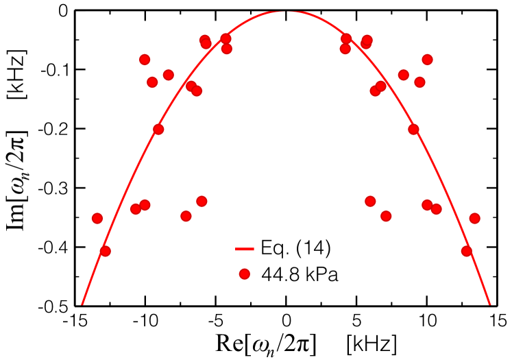
Figure 5: (Color online) Location of the normal mode frequencies in the complex-value plane (Re[$\omega_{n}$], Im[$\omega_{n}$]) which contribute to the pole decomposition Eq. (36) of the data plotted in Fig. 2 for $\sigma=$44.8 kPa. Solid line represents a fit according to the parabolic Eq. (47). This equation neglects the fluctuations in the force distribution, which explains the scattering of the data around the parabolic fit. Other stresses behave similarly.

The locations of the complex-valued normal modes in the $\omega$-plane (Re$[\omega_{n}]$, Im$[\omega_{n}])$ are plotted in Fig. 5 for the tungsten system at $\sigma=44.8$ kPa. The poles are located relatively close to the real axis, indicating that the system is underdamped, Im$[\omega_{n}]\ll$ Re$[\omega_{n}]$, which is consistent with our previous experience JValenza2012 . Furthermore, the data of Fig. 5 of the identified normal modes frequencies follow, in average, a parabolic curve in the complex plane. We have confirmed that this parabolic shape also holds for the other stress levels, however the data is more noisy. This parabolic shape is also confirmed in numerical simulations done in hu .

This result provides the basis for interpreting the experimental data. Indeed, the parabolic curve can be shown to be the result of a weakly damped system with a commutative property of the dynamical matrices: if the damping and stiffness matrices commute, $\mathbf{KB}=\mathbf{BK}$, the trajectories can be approximated by parabolas for small damping. As an illustrative example of this, let us investigate a consequence of the approximation Eq. (23) between the elastic and the damping matrices.

An important implication of Eq. (23) is that the matrices $\mathbf{K}$ and $\mathbf{B}$ commute: $\mathbf{KB}=\mathbf{BK}$, and the set $\{e_{j}^{n}\}$ are the complete eigenvectors for both matrices. The normal modes in the damped system are exactly the same as in the undamped case except that they now have complex-valued frequencies, due to the attenuation. In the presence of damping, each mode exactly decouples.

Expanding Eq. (31) we have,

$$\Big{[}-m\delta_{ij}\omega_{n}^{2}-i\omega_{n}B_{ij}+K_{ij}\Big{]}e_{j}^{n}=0.$$ (42)

When $\xi>$ 0 the normal mode frequencies are complex. If we substitute the approximation Eq. (23) into Eq. (42), we have:

$$\Big{[}-m\delta_{ij}\omega_{n}^{2}-i\omega_{n}\xi K_{ij}+K_{ij}\Big{]}e_{j}^{n}=0.$$ (43)

The approximation Eq. (23) implies that $e_{j}^{n}$ is also an eigenvector of $\mathbf{B}$, which permits us to simplify Eq. (43):

$$-\omega_{n}^{2}-i\xi\omega_{n0}^{2}\omega_{n}+\omega_{n0}^{2}=0,$$ (44)

where $\omega_{n0}$ are the normal modes of the system without damping, $\xi=0$. Equation (44) is a quadratic equation with roots:

$$\omega_{n}=-i\frac{\xi}{2}\omega_{n0}^{2}\pm\omega_{n0}\sqrt{1-\Big{(}\frac{\xi\omega_{n0}}{2}\Big{)}^{2}}.$$ (45)

For large enough damping, $\xi>\xi_{c}=2/\omega_{n0}$, these normal modes are overdamped, and the corresponding frequencies are purely imaginary. For weak damping, $\xi<\xi_{c}$, the modal frequencies are damped oscillators. In this case:

$$\xi<\xi_{c}:\;|\omega_{n}(\xi)|=\omega_{n0}.$$ (46)

Thus, when Eq. (23), the underdamped modes have the property that, for a fixed $\xi\ll\xi_{c}$, the modes lie approximately on a parabola given by:

$$\mbox{Im}[\omega_{n}]\approx-\frac{\xi}{2}\;\mbox{Re}[\omega_{n}]^{2}.$$ (47)

As seen in Fig. 5, the modes exhibit a parabolic shape in the $\omega_{n}$-plane, which suggests the validity of Eq. (47) in average. We fit Eq. (47) to the modal frequencies obtained experimentally in Fig. 5, and find $\xi=(2.2\pm 0.2)\times 10^{-5}$s$\ll\xi_{c}=2/\omega_{n0}$, confirming that the system is weakly damped. We conclude that the scaling of the undamped normal modes can be extracted via Eq. (46), i.e. by plotting the absolute value, $|\omega_{n}|$ against applied stress.

VII Location of the missing modes

At this point we would like to show how the results of our analysis can give an indication of where, in the complex plane, the remaining normal mode frequencies are located. These missing normal mode frequencies correspond to residues which are negligibly small in the measured effective mass and are not visible in the effective mass decomposition. Consider Eq. (45) which may be re-written as

$$[\Re(\omega_{n})]^{2}+[\Im(\omega_{n})+\xi^{-1}]^{2}=\xi^{-2}$$ (48)

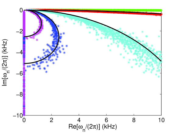
Figure 6: (Color online) Computed complex-valued normal mode frequencies of a simulated system of 400 particles interacting via contact springs and dampers for 5 different values of the damping parameter. From Ref. hu . Although the matrices K and B do not commute in this case, the normal mode frequencies approximately follow the predictions of Eq. (48), which is shown as a solid curve for different values of $\xi$.

Thus, if the matrices B and K commute all the normal mode frequencies, for a fixed value of the damping parameter, $\xi$, lie on a circle of radius $1/\xi$ centered on the point $-i/\xi$, as discussed above. In a separate effort of ours hu we have investigated the extent to which these results may hold true with computer simulations. We have performed molecular dynamic simulations of ensembles of spherical grains in which we take the spring constants, K, to be given by the Hertz-Mindlin theory and we have taken the damping constants, B, to be the same for every non-zero contact. Although B and K do not commute in this case, the computed normal mode frequencies are reasonably well described by the predictions of Eq. (45) as we show in Fig. 6 which is reproduced from hu . Specifically, for each value of the damping parameter, $\xi$, the set $\{\omega_{n}\}$ approximately lies on a circle whose radius decreases as $\xi$ is increased, Eq. (48). The matrices B and K are mostly zero-valued, except for grains which are actually in contact with each other. In this sense we may say that they approximately commute; hence Eqs. (46) and (48) are approximately true.

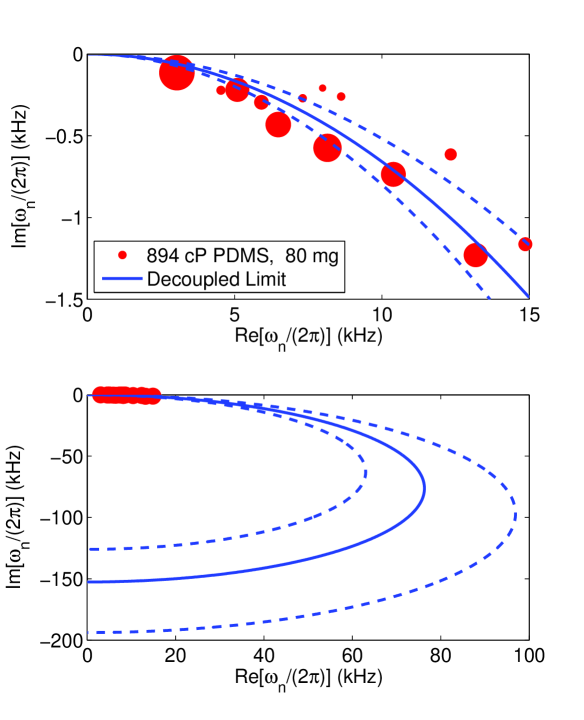
Figure 7: (Color online) (a) Complex-valued normal mode frequencies determined from experimental data of loose granular tungsten particles, lightly coated with 80 mg of PDMS of viscosity 894 cP. From Ref JValenza2012 . This system is identical to the system of Fig. 5 except for larger amount of PDMS which increases the dissipation. The size of each symbol is proportional to the magnitude of the residue, $A_{n}$, in the decomposition of the effective mass data. The solid curve is a best fit of the data to Eq. (48). The dashed curves are for radius values corresponding to the full width at double the minimum of the cost function, Eq. (49). (b) Same as (a) but with an expanded scale. We expect the missing normal mode frequencies - those whose residues are negligibly small in the measured effective mass - to lie within these bands or on the negative imaginary axis.

We suppose these features also apply to real data on real granular media as we have already seen in Fig. 5. In order to draw some quantitative conclusions from our data we replot, in Fig. 7, some of our previously published results JValenza2012 which were deduced from the measured effective mass of tungsten granules lightly coated with viscous PDMS fluid. The difference between the system of coated tungsten particles used in Fig. 5 and Fig. 7 is that in the later we use larger amount of silicone oil to coat the particles (80 mg as indicated). Thus, the damping in the system is increased as shown in JValenza2012 . We have fit the data to Eq. (48) using the cost function

$$\chi(R)=\sum_{n}\mid A_{n}\mid r_{n}^{2}\;[\theta_{n}-\theta(r_{n};R)]^{2}\>\>\>.$$ (49)

Here, $R=1/\xi$ is the radius of the circle and the resonant frequencies are written in polar coordinates: $\omega_{n}=r_{n}\exp{(i\theta_{n})}$. $A_{n}$ are the residues of the poles in the decomposition of the effective mass data, Eq. (36); their magnitudes are indicated by the sizes of the symbols in Fig. 7. $\theta(r;R)=-\arcsin(r/2R)$ is the representation of Eq. (48) in polar coordinates. The results are shown in Fig. 7(a).

Although the existing data cover only a small arc of the circle, we feel that based on the results of our numerical simulations, and the fact that the existing data do trend along the curve, Eq. (48), we may conclude that the underdamped resonance frequencies which we are not able to directly locate with our effective mass measurements lie roughly between the bounds of the two dashed curves in Fig. 7. The overdamped resonance frequencies will lie on the negative imaginary axis, of course.

VIII Stress-dependence of the characteristic frequency

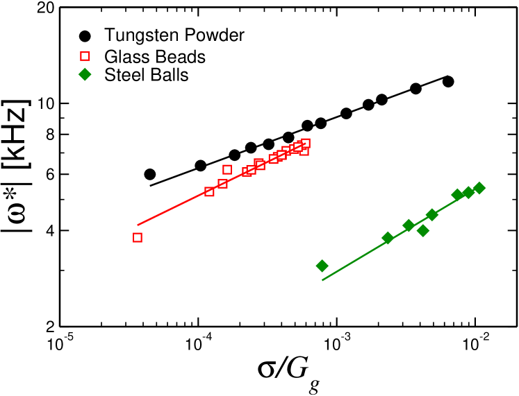
Figure 8: (Color online) Absolute value of the characteristic frequency, $|\omega^{*}(\sigma)|$, corresponding to the main resonance peak of the effective mass as a function of stress $\sigma$ rescaled by the shear modulus ($G_{g}$) of the material from which the particles are made. We plot results for experimental systems composed of tungsten irregular particles of $\sim 150\mu$m coated with PDMS, uncoated spherical glass beads of 1mm, uncoated steel balls of 2mm. Solid lines are power-law fits with OLS estimator. Exponents are reported in Table 1.

The pole with the largest residue contributing to the resonance frequency at the main peak of the effective mass defines the characteristic frequency $|\omega^{*}(\sigma)|$. By the absolute value we indicate that this is the characteristic frequency of the damped modes obtained via the effective mass to distinguish it from the undamped $\omega_{D}^{*}$ obtained from the Debye departure in the density of states in Eq. (1). Figure 8 shows $|\omega^{*}(\sigma)|$ indicating a power-law dependence on $\sigma$ consistent with Eq. (1) for the tungsten powder. Using an OLS estimator, we find $\Omega^{\prime}=0.15\pm 0.02$ ($R^{2}=0.9949$). More specifically, the fitting yields:

$$|\omega^{*}(\sigma)|=(3.27\pm 0.03)\,\sigma^{\Omega^{\prime}},$$ (50)

with $\sigma$ measured in kPa and the frequency in kHz.

Using the stress vs strain curve in Fig. 3a with $\alpha=1.15\pm 0.01$, we find $\Omega=0.17\pm 0.02$ and $\delta=0.10\pm 0.02$ for the tungsten powder.

We test further the results with packings constituted by different particle types. We use spherical particles made of glass beads (1mm diameter) and steel balls (2mm diameter) without coating. Figure 8 shows the scaling of $|\omega^{*}|$ with stress for these systems and the exponents ($\Omega^{\prime},\Omega,\delta,\alpha$) are indicated in Table 1 (see Fig. 3b for constitutive law). We find for glass beads $\delta=0.14\pm 0.02$ and for steel balls $\delta=0.13\pm 0.02$.

The exponent of the tungsten particles is smaller than the rest. We hypothesize that irregularities in particle shape may add some complexity in the modes not seen in spherical particles. These particles were obtained by fusing two or three irregular (approximately cubic) particles with facets and angularities that may introduce modes not seen in spherical particles coupling the rotational and translational modes in an uncontrolled way.

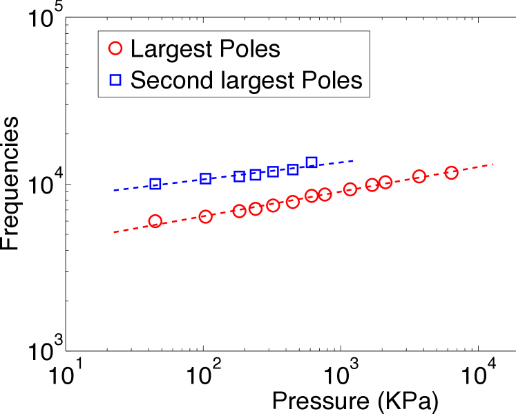
Figure 9: (Color online) Scaling of the modes obtained from the first and second peak of the tungsten system showing similar scaling with pressure.

We also test the scaling of the other modes obtained from the effective mass by looking at the modes with smaller residue than the main characteristic frequency. We find that the other modes scale with similar exponent as the characteristic mode $|\omega^{*}|$ (Fig. 9). The lack of data in the second peak for large stress is due to the fact that they fall outside of our experimental range of observation for high enough pressures. This is also corroborated by the data collapse shown in Fig. 2c and 2d. The result of the characteristic frequency following a decreasing path in stress is plotted in Fig. 10 showing that the scaling of the characteristic frequency with stress yields similar exponent as the upward path in stress shown in Fig. 8.

IX Conclusions

Our results suggest that granular materials near jamming behave critically with a characteristic frequency defined by a critical exponent $\delta$. The experimental exponents $\delta$ are consistently smaller than $\delta_{\rm th}=1/2$ predicted by theory Matthieu2005 ; Wyart2005 . Such an anomalous exponent $\delta<1/2$ poses new theoretical challenges to explain frictional systems with translational and rotational degrees of freedom. It might be possible that the path followed in stress space may change the value of the exponents. The usual path followed in previous works is along the line of zero shear stress, as a function of packing fraction. The present experiments follow a line of changing uniaxial stress, which would place it along a path that excites bulk and shear modes. Thus, it is plausible that the exponents might be affected by the path taken to approach the jamming transition. Another interpretation is that the lowest of our frequencies may not be a proxy for the cutoff frequency $\omega_{D}^{*}$, which separates the region of excess density of states from the Debye region. However, if some universality could be claimed at the jamming transition, both characteristic frequencies should scale with stress with the same universal exponent. In the same line, it is interested to note that the lowest frequency estimated from the effective mass is directly obtained from the dynamical matrix as done in $\omega_{D}^{*}$ as well.

In general, other mechanical properties such as elastic constants (shear and bulk moduli), sound speeds, and attenuation can be obtained from the effective mass measurement Chaur2009 ; JValenza2012 . Furthermore, the theory can be extended to non-spherical particles as well Baule2 .Thus, the effective mass technique facilitates a systematic test of the scaling laws of the anomalous mechanical and acoustic properties of athermal and dissipative granular systems near the jamming transition. We hope that this technique may open new experimental tests of granular matter near the jamming point.

Acknowledgements. We acknowledge funding by DOE Office of Basic Energy Sciences, Geosciences Division, Grant DE-FG02-03ER15458. This work was partially supported by NSF-CMMT. We are grateful to S. Reis and E. Kyeyune-Nyombi for help with experiments and simulations. F. Santibanez acknowledges FONDECYT POSTDOC project N^o 3120130.

Material	Size	Shape	Damping	$\Omega^{\prime}$	$\alpha$	$\Omega=\alpha\Omega^{\prime}$	$\delta$
Tungsten powder	$\sim 150\mu$m	irregular	coating	0.15	1.15	0.17	0.10
Glass beads	1 mm	sphere	no coating	0.21	1.25	0.26	0.14
Steel balls	2 mm	sphere	no coating	0.195	1.21	0.24	0.13
Theory linear spring Wyart2005	–	sphere	–	1/2	1	1/2	1/2
Theory Hertz Wyart2005	–	sphere	–	1/2	3/2	3/4	1/2

Table 1: Summary of the measured exponents and predicted by theory.

X Appendix. Experimental set up

We characterize the normal mode spectrum of the granular medium by measuring the effective mass. The main results in the text are for a granular medium made of tungsten powder that is lightly coated with silicone oil (PDMS) of viscosity 894 cP. We also present results for spherical glass beads of 1 mm diameter and spherical steel balls of 2mm. Both systems are uncoated. The preparation protocol is the same for all cases. Below, we explain the experimental procedure for tungsten particles.

The tungsten powder JValenza2009 and coating procedure JValenza2012 are discussed elsewhere. In the latter reference we found that the light PDMS coating significantly dampened or eliminated the low amplitude modes in the system. This is advantageous for the purposes of this study because it permits us to unambiguously monitor the effect of pressure on the trajectory of the dominant large amplitude modes in the system. The purpose of using tungsten as a material for the particles is to achieve a large mass of the granular system in comparison with the mass of the cup, to maximize the difference between both quantities and obtain a reliable effective mass.

After coating, $\sim$100 g of the weakly wet powder is poured into a cylindrical cup (Fig. 1). The cup has internal diameter=2.54 cm, and height=3.08 cm. The sides of the cup are tapped to encourage the powder to settle, and yield a flat free surface. Finally, the system is compacted using a cyclical stress imposed with an Inkstrom press of sequentially increasing then decreasing amplitude as we have previously developed brujic . The maximum stress amplitude is 118.5 kPa. It was previously shown JValenza2009 that this handling procedure suitably produces a finite sized granular medium with a reproducible effective mass which is independent on the amplitude of oscillation. The mechanical compaction protocol is discussed in detail in reference JValenza2009 .

The effective mass measurement is discussed in reference Chaur2009 ; JValenza2009 ; JValenza2012 . The cylindrical cup is subjected to a vertical, sinusoidal displacement where the vibrational frequency is varied in the range 0.1 - 15 kHz. We take frequency steps of 10 Hz, and at each frequency we measure the force on the bottom of the cup, and the acceleration at two points on opposite ends of a single diameter. The mass is determined by the difference between the ratio of the force to the average acceleration, and the static mass of the cup. The effective mass is a frequency dependent complex value, owing to the partial in phase partial out of phase motion of the individual grains.

The objective of this work is to observe the effect of a uniaxial confining pressure on the dominant normal modes in our granular system. To impose a sequentially increasing stress on the granular medium, we place a thin $\sim$ 5 - 8 mm urethane plug on the free surface of the powder, and screw a cap on top of the cup. After determining the orientation of the cap corresponding to initial contact with the top of the urethane, we further tighten the cap to impose a uniaxial compressive stress. Each rotation of the cap corresponds to an axial displacement that is governed by the characteristics of the threads which support the cap. To convert this displacement to a stress, we use a mechanical testing machine to characterize the stress-displacement relationship of the coupled urethane/tungsten powder system in the cup.

The results of the effective mass are shown in Fig. 2. It is visually apparent from Fig. 2 that only a few modes appear in the effective mass while 12N modes are expected. The effective mass is sensitive to the extended modes in the system corresponding to collective motion of the grains. For instance, the main mode from where we obtain the characteristic frequency, is an extended mode spanning the system size. The remaining modes are more localized, correspond to modes with smaller residues, or are heavily damped and are difficult to observe them in the shape of the effective mass. However, all the 12N modes appear in the effective mass measurement. The remaining modes, being more damped, do not show easily in the shape of the effective mass. Thus, the effective mass is most effective in finding the main extended modes in the system.

Thus, modes with small residues are difficult to see in the effective mass since they are overshadowed by the extended modes with larger residues appearing as large peaks in Im($\omega$). This picture is corroborated in the pole analysis of Fig. 4. When we subtract the main pole contribution of the characteristic frequency $|\omega^{*}|$, a finer structure with many small peaks (called Remainder in Fig. 4) appears. This finer structure corresponds to the remainder modes with smaller residues. By subtracting one by one the contribution of these modes from the effective mass, in principle, we could obtain the entire subset of the 12N modes that appear in the window of observation. In practice, we do it for only the few largest modes since we are interested in the extended modes that test the criticality of the system. However, the procedure can be extended to find more modes until a given resolution preset by the experimental measurement of the effective mass. That is, one can continue extracting modes from the pole decomposition as long as the mass measurement can resolve the peaks in the Reminder of the effective mass.

Thus, while nonlinearities are inherent in the system, still the 12N modes are part of the effective mass, at least those that are within the experimental window of observation. As long as the sought-after poles lie within the rectangle [$\pm 15$ kHz, $\pm i$15 kHz], our procedure will determine their properties with a reasonable accuracy.

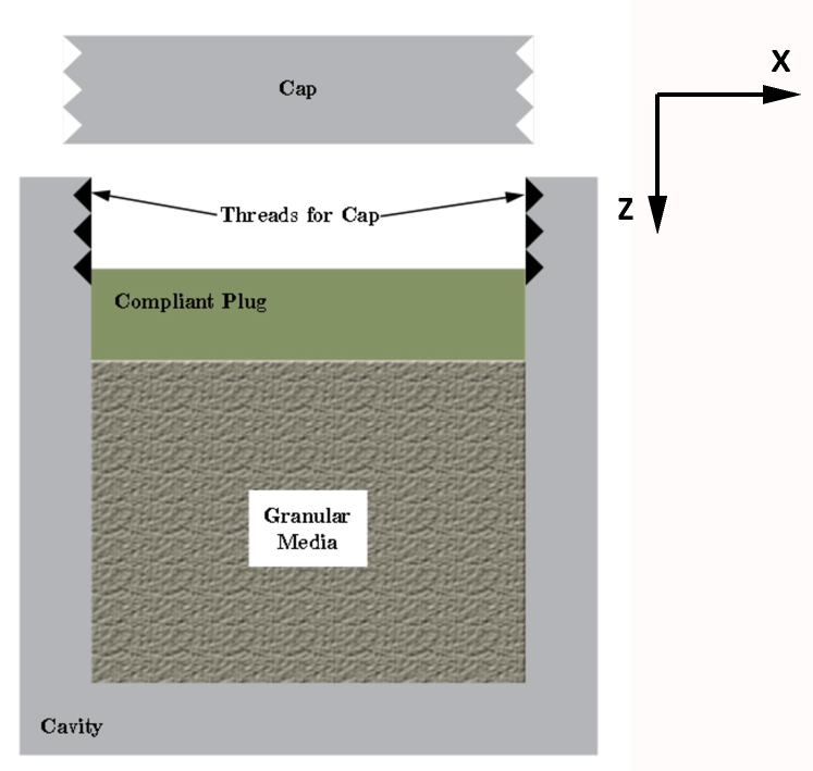
Figure 1: (Color online) Schematic of cup used in effective mass experiments. A compliant plug is sandwiched between the tungsten powder and the cap. The uniaxial confining stress is increased by tightening the cap.

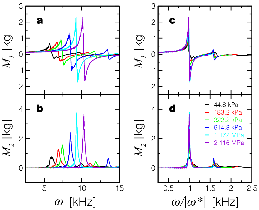
Figure 2: (Color online) Effective mass of tungsten particles in a cup as a function of driving frequency: (a) Real part $M_{1}(\omega)$, and (b) Imaginary part, $M_{2}(\omega)$, plotted for the indicated external stresses. We calculate $\tilde{M}$ for 13 stresses between $\sigma=44.8$ kPa and 6.39 MPa and show six curves as indicated for clarity. All datasets are available at http://jamlab.org. (c)-(d) Data collapse of $M_{1}(\omega)$ and $M_{2}(\omega)$ according to the scaling scenario Eq. (1).

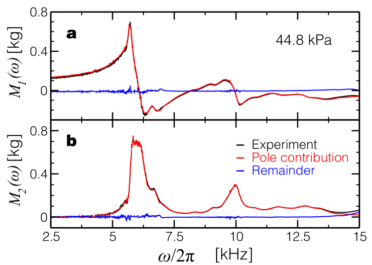
Figure 4: (Color online) Pole decomposition. Comparison of pole decomposition using Eq. (36) and the obtained poles and experimental data at 44.8 kPa for the tungsten particles. We also plot the difference showing that many more nodes with small residues are still present in the effective mass.

Figure 10: Test of reversibility in the glass beads experimental system. We follow a decreasing path in pressure and obtain similar exponent $\Omega^{\prime}=0.20\pm 0.02$ as the one obtained with the upward pressure path reported in Table 1.

References

- (1) A. L. Liu, S. R. Nagel, (eds.), Jamming and Rheology: Constrained Dynamics on Microscopic and Macroscopic Scales (Taylor & Francis, London, 2001).
- (2) S. Alexander, Phys. Rep. 296, 65 (1998).
- (3) C. F. Moukarzel, Phys. Rev. Lett. 81, 1634 (1998).
- (4) H. A. Makse, D. L. Johnson, L. M. Schwartz, Phys. Rev. Lett. 84, 4160 (2000).
- (5) C. S. O’Hern, S. A. Langer, A. J. Liu, S. R. Nagel, Phys. Rev. Lett. 88, 075507 (2002).
- (6) M. Wyart, S. R. Nagel, T. A. Witten, Europhys. Lett. 72, 486 (2005).
- (7) M. Wyart, L. E. Silbert, S. R. Nagel T. Witten, Phys. Rev. E 72, 051306 (2005).
- (8) A. J. Liu, S. R. Nagel, W. van Saarloos, M. Wyart, The jamming scenario - an introduction and outlook, in Dynamical Heterogeneities in Glasses, Colloids, and Granular Media (Oxford University Press, 2011).
- (9) C. S. O’Hern, L. E. Silbert, A. J. Liu, S. R. Nagel, Phys. Rev. E 68, 011306 (2003).
- (10) L. E. Silbert, A. J. Liu, S. R. Nagel, Phys. Rev. Lett. 95, 098301 (2005).
- (11) E. Somfai, M. van Hecke, W. G. Ellenbroek, K. Shundyak, W. van Saarloos, Phys. Rev. E 75, 020301R (2007).
- (12) N. Xu, M. Wyart, A. J. Liu, S. R. Nagel, Phys Rev. Lett 98, 175502 (2007).
- (13) H. Zhang, H. A. Makse, Phys. Rev. E 72, 011301 (2005).
- (14) J. Brujić, C. Song, P. Wang, C. Briscoe, G. Marty, H. A. Makse, Phys. Rev. Lett. 98, 248001 (2007).
- (15) A. Ghosh, et al. Phys. Rev. Lett. 104, 248305 (2010).
- (16) K. Chen, et al. Phys. Rev. Lett. 105, 025501 (2010).
- (17) A. Widmer-Cooper, H. Perry, P. Harrowell, D. R. Reichman, Nature Phys. 4, 711 (2008).
- (18) C.-J. Hsu, et al. Phys. Rev. Lett. 102, 058001 (2008).
- (19) J. J. Valenza, et al. Phys. Rev. E 80, 051304 (2009).
- (20) J. J. Valenza, D. L. Johnson, Phys. Rev. E 85, 041302 (2012).
- (21) J. Brujić, P. Wang, C. Song, D. L. Johnson, O. Sindt, and H. A. Makse, Phys. Rev. Lett. 95, 128001 (2005).
- (22) H. A. Makse, J. Brujić, and S. F. Edwards, “Statistical Mechanics of Jammed Matter”, in The Physics of Granular Media, edited by H. Hinrichsen and D. E. Wolf, (Wiley-VCH), (2004).
- (23) C. Briscoe, C. Song, P. Wang, and H. A. Makse, Phys. Rev. Lett. 101, 188001 (2008).
- (24) A. Baule, H. A. Makse. Fundamental challenges in packing problems: from spherical to non-spherical particles. Soft Matter, DOI: 10.1039/c3sm52783b (2014).
- (25) N. K. Brilliantov, F. Spahn, J.-M. Hertzsch, T. Poschel, Phys. Rev. E 53, 5382 (1996).
- (26) J. Shafer, S. Dippel, D. E. Wolf, J. Phys. I (France) 6, 5- (1996).
- (27) G. Kuwabara, K. Kono, Jap. J. Appl. Phys. 26, 1230 (1987).
- (28) L. D. Landau, E. M. Lifshitz, E. M. Theory of Elasticity (Oxford University Press, Oxford, 1965).
- (29) H. A. Makse, N. Gland, D. L. Johnson, L. M. Schwartz, Phys. Rev. E 70, 061302 (2004).
- (30) D. J. Inman, A. N. Andry, J. Appl. Mech. 47, 927 (1980).
- (31) A. Bhaskar, J. Appl. Mech. 64, 387 (1997).
- (32) J. H. Wilkinson, Algebraic Eigenvalue Problem (Oxford University Press, New York, 1965).
- (33) W. J. Tzeng, F. Y. Wu, J. Phys. A: Math. Gen. 39, 8579 (2006).
- (34) J. Stoer, R. Bulirsch, R. Introduction to Numerical Analysis (3rd ed.) (Springer, New York, 2002).
- (35) W. H. Press, B. P. Flannery, S. A. Teukolsky, W. T. Vetterling, Numerical Recipes (Cambridge University Press, New York, 1987).
- (36) Y. Hu, H. A. Makse, J. J. Valenza, D. L. Johnson, Geophysics (2014).
- (37) A. Baule, R. Mari, L. Bo. L. Portal, H. A. Makse, ”Mean-field theory for random close packings of axisymmetric particles”,Nature Communications 4 , 2194 (2013).