Thermal properties of light tensor mesons via QCD sum rules

The thermal properties of $f_{2}(1270)$, $a_{2}(1320)$ and $K_{2}^{*}(1430)$ light tensor mesons are investigated in the framework of QCD sum rules at finite temperature. In particular, the masses and decay constants of the light tensor mesons are calculated taking into account the new operators appearing at finite temperature. The numerical results show that at the point which the temperature-dependent continuum threshold vanishes, the decay constants decrease with amount of $(70-85)\%$ compared to their vacuum values, while the masses diminish about $(60-72)\%$ depending on the kinds of the mesons under consideration. The results obtained at zero temperature are in good consistency with the experimental data as well as existing theoretical predictions.

PACS number(s): 11.10.Wx, 11.55.Hx, 14.40.Be, 14.40.Df

1 Introduction

The study of strong interaction at low energies is one of the most important problems of the high energy physics. This can play a crucial role to explore the structure of mesons, baryons and vacuum properties of strong interaction. The tensor particles can provide a different perspective for understanding the low energy QCD dynamics. In recent decades there have been made great efforts both experimentally and theoretically to investigate the tensor particles in order to understand their nature and internal structure.

The investigation of hadronic properties at finite baryon density and temperature in QCD also plays an essential role for interpretation of the results of heavy-ion collision experiments and obtaining the QCD phase diagram. The Compressed Baryonic Matter (CBM) experiment of the FAIR project at GSI is important for understanding the way of Chiral symmetry realization in the low energy region and, consequently, the confinement of QCD. According to thermal QCD, the hadronic matter undergoes to quark gluon-plasma phase at a critical temperature. These kind of phase may exist in the neutron stars and early universe. Hence, calculation of the parameters of hadrons via thermal QCD may provide us with useful information on these subjects.

The restoration of Chiral symmetry at high temperature requires the medium modifications of hadronic parameters [1]. There are many non-perturbative approaches to hadron physics. The QCD sum rule method [2, 3] is one of the most attractive and applicable tools in this respect. In this approach, hadrons are represented by their interpolating quark currents and the correlation function of these currents is calculated using the operator product expansion (OPE). The thermal version of this approach is based on some basic assumptions so that the Wilson expansion and the quark-hadron duality approximation remain valid, but the vacuum condensates are replaced by their thermal expectation values [4]. At finite temperature, the Lorentz invariance is broken and due to the residual $O(3)$ symmetry, some new operators appear in the Wilson expansion [5, 6, 7]. These operators are expressed in terms of the four-vector velocity of the medium and the energy momentum tensor. There are numerous works in the literature on the medium modifications of parameters of (psedo)scalar and (axial)vector mesons using different theoretical approaches e.g. Chiral model [8], coupled channel approach [9, 10] and QCD sum rules [5, 6, 11, 12, 13, 14, 15, 16, 17]. Recently, we applied this method to calculate some hadronic parameters related to the charmed $D_{2}^{*}(2460)$ and charmed-strange $D_{s2}^{*}(2573)$ tensor [18] mesons.

In the present work we investigate the properties of light $a_{2}(1320)$, $f_{2}(1270)$ and $K_{2}^{*}(1430)$ tensor mesons in the framework of QCD sum rules at finite temperature. We also compare the results obtained at zero temperature with the predictions of some previous studies on the parameters of the same mesons in vacuum [19, 20, 21].

The present article is organized as follows. In next section, considering the new operators raised at finite temperature, we evaluate the corresponding thermal correlation function to obtain the QCD sum rules for the parameters of the mesons under consideration. Last section is devoted to the numerical analysis of the sum rules obtained as well as investigation of the sensitivity of the masses and decay constants of the light tensor mesons on temperature.

2 Thermal QCD Sum Rules for Masses and Decay Constants of Light Tensor Mesons

In this section we present the basics of the thermal QCD sum rules and apply this method to some light tensor mesons like $f_{2}(1270)$, $a_{2}(1320)$ and $K_{2}^{*}(1430)$ to compute their mass and decay constant. The starting point is to consider the following thermal correlation function:

$$\Pi_{\mu\nu,\alpha\beta}(q,T)=i\int d^{4}xe^{iq\cdot(x-y)}Tr\left\{\rho{\cal T}\left[J_{\mu\nu}(x)\overline{J}_{\alpha\beta}(y)\right]\right\},$$ (1)

where $\rho=e^{-\beta H}/Tr(e^{-\beta H})$ is the thermal density matrix of QCD, $\beta=1/T$ with $T$ being temperature, $H$ is the QCD Hamiltonian, ${\cal T}$ indicates the time ordered product and $J_{\mu\nu}$ is the interpolating current of tensor mesons. The interpolating fields for these mesons can be written as

$$J_{\mu\nu}^{K_{2}^{*}}(x)=\frac{i}{2}\left[\bar{s}(x)\gamma_{\mu}\stackrel{{\scriptstyle\leftrightarrow}}{{\cal D}}_{\nu}(x)d(x)+\bar{s}(x)\gamma_{\nu}\stackrel{{\scriptstyle\leftrightarrow}}{{\cal D}}_{\mu}(x)d(x)\right],$$ (2)

$$J_{\mu\nu}^{f_{2}}(x) = \frac{i}{2\sqrt{2}}\Big{[}\bar{u}(x)\gamma_{\mu}\stackrel{{\scriptstyle\leftrightarrow}}{{\cal D}}_{\nu}(x)u(x)+\bar{u}(x)\gamma_{\nu}\stackrel{{\scriptstyle\leftrightarrow}}{{\cal D}}_{\mu}(x)u(x)$$ (3)

$$+ \bar{d}(x)\gamma_{\mu}\stackrel{{\scriptstyle\leftrightarrow}}{{\cal D}}_{\nu}(x)d(x)+\bar{d}(x)\gamma_{\nu}\stackrel{{\scriptstyle\leftrightarrow}}{{\cal D}}_{\mu}(x)d(x)\Big{]},$$

and

$$J_{\mu\nu}^{a_{2}}(x) = \frac{i}{2\sqrt{2}}\Big{[}\bar{u}(x)\gamma_{\mu}\stackrel{{\scriptstyle\leftrightarrow}}{{\cal D}}_{\nu}(x)u(x)+\bar{u}(x)\gamma_{\nu}\stackrel{{\scriptstyle\leftrightarrow}}{{\cal D}}_{\mu}(x)u(x)$$ (4)

$$- \bar{d}(x)\gamma_{\mu}\stackrel{{\scriptstyle\leftrightarrow}}{{\cal D}}_{\nu}(x)d(x)-\bar{d}(x)\gamma_{\nu}\stackrel{{\scriptstyle\leftrightarrow}}{{\cal D}}_{\mu}(x)d(x)\Big{]},$$

where $\stackrel{{\scriptstyle\leftrightarrow}}{{\cal D}}_{\mu}(x)$ denotes the derivative with respect to four-$x$ simultaneously acting on left and right. It is given as

$$\stackrel{{\scriptstyle\leftrightarrow}}{{\cal D}}_{\mu}(x)=\frac{1}{2}\left[\stackrel{{\scriptstyle\rightarrow}}{{\cal D}}_{\mu}(x)-\stackrel{{\scriptstyle\leftarrow}}{{\cal D}}_{\mu}(x)\right],$$ (5)

where

$$\overrightarrow{{\cal D}}_{\mu}(x)=\overrightarrow{\partial}_{\mu}(x)-i\frac{g}{2}\lambda^{a}A^{a}_{\mu}(x),$$

$$\overleftarrow{{\cal D}}_{\mu}(x)=\overleftarrow{\partial}_{\mu}(x)+i\frac{g}{2}\lambda^{a}A^{a}_{\mu}(x),$$ (6)

with $\lambda^{a}(a=1,8)$ and $A^{a}_{\mu}(x)$ are being the Gell-Mann matrices and external gluon fields, respectively. The currents contain derivatives with respect to the space-time, hence we consider the two currents at points $x$ and $y$ in Eq. (1), but for simplicity, we will set $y=0$ after applying derivative with respect to $y$.

It is well known that in thermal QCD sum rule approach, the thermal correlation function can be calculated in two different ways. Firstly, it is calculated in terms of hadronic parameters such as masses and decay constants. Secondly, it is calculated in terms of the QCD parameters such as quark masses, quark condensates and quark-gluon coupling constants. The coefficients of sufficient structures from both representations of the same correlation function are then equated to find the sum rules for the physical quantities under consideration. We apply Borel transformation and continuum subtraction to both sides of the sum rules in order to further suppress the contributions of the higher states and continuum.

Let us focus on the calculation of the hadronic side of the correlation function. For this aim we insert a complete set of intermediate physical state having the same quantum numbers as the interpolating current into Eq. (1). After performing integral over four-$x$ and setting $y=0$, we get

$$\Pi_{\mu\nu,\alpha\beta}(q,T)=\frac{{\langle}0\mid J_{\mu\nu}(0)\mid K_{2}^{*}(f_{2})(a_{2})\rangle\langle K_{2}^{*}(f_{2})(a_{2})\mid\bar{J}_{\alpha\beta}(0)\mid 0\rangle}{m_{K_{2}^{*}(f_{2})(a_{2})}^{2}-q^{2}} + \cdots,$$ (7)

where dots indicate the contributions of the higher and continuum states. The matrix element $\langle 0\mid J_{\mu\nu}(0)\mid K_{2}^{*}(f_{2})(a_{2})\rangle$ creating the tensor mesons from vacuum can be written in terms of the decay constant, $f_{K_{2}^{*}(f_{2})(a_{2})}$ as

$$\langle 0\mid J_{\mu\nu}(0)\mid K_{2}^{*}(f_{2})(a_{2})\rangle=f_{K_{2}^{*}(f_{2})(a_{2})}m_{K_{2}^{*}(f_{2})(a_{2})}^{3}\varepsilon^{(\lambda)}_{\mu\nu},$$ (8)

where $\varepsilon^{(\lambda)}_{\mu\nu}$ is the polarization tensor. Using Eq. (8) in Eq. (7), the final expression of the physical side is obtained as

$$\Pi_{\mu\nu,\alpha\beta}(q,T)=\frac{f_{K_{2}^{*}(f_{2})(a_{2})}^{2}m_{K_{2}^{*}(f_{2})(a_{2})}^{6}}{m_{K_{2}^{*}(f_{2})(a_{2})}^{2}-q^{2}}\left\{\frac{1}{2}(g_{\mu\alpha}g_{\nu\beta}+g_{\mu\beta}g_{\nu\alpha})\right\}+\mbox{other structures}+...,$$ (9)

where the only structure that we will use in our calculations has been shown explicitly. To obtain the above expression we have used the summation over polarization tensors as

$$\sum_{\lambda}\varepsilon_{\mu\nu}^{(\lambda)}\varepsilon_{\alpha\beta}^{*(\lambda)}=\frac{1}{2}T_{\mu\alpha}T_{\nu\beta}+\frac{1}{2}T_{\mu\beta}T_{\nu\alpha}-\frac{1}{3}T_{\mu\nu}T_{\alpha\beta},$$ (10)

where

$$T_{\mu\nu}=-g_{\mu\nu}+\frac{q_{\mu}q_{\nu}}{m_{K_{2}^{*}(f_{2})(a_{2})}^{2}}.$$ (11)

Now we concentrate on the OPE side of the thermal correlation function. In OPE representation, the coefficient of the selected structure can be separated into perturbative and non-perturbative parts

$$\Pi(q,T)=\Pi^{pert}(q,T)+\Pi^{non-pert}(q,T).$$ (12)

The perturbative or short-distance contributions are calculated using the perturbation theory. This part in spectral representation is written as

$$\Pi^{pert}(q,T)=\int ds\frac{\rho(s)}{s-q^{2}},$$ (13)

where $\rho(s)$ is the spectral density and it is given by the imaginary part of the correlation function, i.e.,

$$\rho(s)=\frac{1}{\pi}Im[\Pi^{pert}(s,T)].$$ (14)

The non-perturbative or long-distance contributions are represented in terms of thermal expectation values of the quark and gluon condensates as well as thermal average of the energy density. Our main task in the following is to calculate the spectral density as well as the non-perturbative contributions. For this aim we use the explicit forms of the interpolating currents for the tensor mesons in Eq. (1). After contracting out all quark fields using the Wick’s theorem, we get

$$\Pi_{\mu\nu,\alpha\beta}^{K_{2}^{*}}(q,T) = -\frac{i}{4}\int d^{4}xe^{iq\cdot(x-y)}\Bigg{\{}Tr\Big{[}S_{s}(y-x)\gamma_{\mu}\stackrel{{\scriptstyle\leftrightarrow}}{{\cal D}}_{\nu}(x)\stackrel{{\scriptstyle\leftrightarrow}}{{\cal D}}_{\beta}(y)S_{d}(x-y)\gamma_{\alpha}\Big{]}$$ (15)

$$+ \left[\beta\leftrightarrow\alpha\right]+\left[\nu\leftrightarrow\mu\right]+\left[\beta\leftrightarrow\alpha,\nu\leftrightarrow\mu\right]\Bigg{\}},$$

and

$$\Pi_{\mu\nu,\alpha\beta}^{f_{2}(a_{2})}(q,T) = -\frac{i}{8}\int d^{4}xe^{iq\cdot(x-y)}\Bigg{\{}Tr\Big{[}S_{u}(y-x)\gamma_{\mu}\stackrel{{\scriptstyle\leftrightarrow}}{{\cal D}}_{\nu}(x)\stackrel{{\scriptstyle\leftrightarrow}}{{\cal D}}_{\beta}(y)S_{u}(x-y)\gamma_{\alpha}$$ (16)

$$+ S_{d}(y-x)\gamma_{\mu}\stackrel{{\scriptstyle\leftrightarrow}}{{\cal D}}_{\nu}(x)\stackrel{{\scriptstyle\leftrightarrow}}{{\cal D}}_{\beta}(y)S_{d}(x-y)\gamma_{\alpha}\Big{]}+\left[\beta\leftrightarrow\alpha\right]+\left[\nu\leftrightarrow\mu\right]$$

$$+ \left[\beta\leftrightarrow\alpha,\nu\leftrightarrow\mu\right]\Bigg{\}}.$$

To proceed we need to know the thermal light quark propagator $S_{q=u,d,s}(x-y)$ in coordinate space which is given as [18, 22]:

$$S_{q}^{ij}(x-y) = i\frac{\!\not\!{x}-\!\not\!{y}}{2\pi^{2}(x-y)^{4}}\delta_{ij}-\frac{m_{q}}{4\pi^{2}(x-y)^{2}}\delta_{ij}-\frac{\langle\bar{q}q\rangle}{12}\delta_{ij}-\frac{(x-y)^{2}}{192}m_{0}^{2}\langle\bar{q}q\rangle\Big{[}1-i\frac{m_{q}}{6}(\!\not\!{x}-\!\not\!{y})\Big{]}\delta_{ij}$$ (17)

$$+ \frac{i}{3}\Big{[}(\!\not\!{x}-\!\not\!{y})\Big{(}\frac{m_{q}}{16}\langle\bar{q}q\rangle-\frac{1}{12}\langle u\Theta^{f}u\rangle\Big{)}+\frac{1}{3}\Big{(}u\cdot(x-y)\!\not\!{u}\langle u\Theta^{f}u\rangle\Big{)}\Big{]}\delta_{ij}$$

$$- \frac{ig_{s}}{32\pi^{2}(x-y)^{2}}G_{\mu\nu}\Big{(}(\!\not\!{x}-\!\not\!{y})\sigma^{\mu\nu}+\sigma^{\mu\nu}(\!\not\!{x}-\!\not\!{y})\Big{)}\delta_{ij},$$

where $\langle\bar{q}q\rangle$ is the temperature-dependent quark condensate, $\Theta^{f}_{\mu\nu}$ is the fermionic part of the energy momentum tensor and $u_{\mu}$ is the four-velocity of the heat bath. In the rest frame of the heat bath, $u_{\mu}=(1,0,0,0)$ and $u^{2}=1$.

The next step is to use the expressions of the propagators and apply the derivatives with respect to $x$ and $y$ in Eqs. (15) and (16). After lengthy but straightforward calculations the spectral densities at different channels are obtained as

$$\rho_{K_{2}^{*}}(s)=N_{c}\Big{(}\frac{m_{d}m_{s}s}{32\pi^{2}}+\frac{s^{2}}{160\pi^{2}}\Big{)},$$ (18)

and

$$\rho_{f_{2}(a_{2})}(s)=N_{c}\Big{(}\frac{(m_{u}^{2}+m_{d}^{2})s}{96\pi^{2}}+\frac{s^{2}}{160\pi^{2}}\Big{)},$$ (19)

where $N_{c}=3$ is the number of colors. From a similar way, for the non-perturbative contributions we get

$$\Pi^{non-pert}_{K_{2}^{*}}(q,T)=\frac{(6m_{s}-5m_{d})m_{0}^{2}}{144q^{2}}\langle\bar{d}d\rangle+\frac{(6m_{d}-5m_{s})m_{0}^{2}}{144q^{2}}\langle\bar{s}s\rangle-\frac{2\langle u\Theta^{f}u\rangle(q\cdot u)^{2}}{9q^{2}},$$ (20)

and

$$\Pi^{non-pert}_{f_{2}(a_{2})}(q,T)=\frac{m_{d}m_{0}^{2}}{144q^{2}}\langle\bar{d}d\rangle+\frac{m_{u}m_{0}^{2}}{144q^{2}}\langle\bar{u}u\rangle-\frac{2\langle u\Theta^{f}u\rangle(q\cdot u)^{2}}{9q^{2}}.$$ (21)

After matching the hadronic and OPE representations, applying Borel transformation with respect to $q^{2}$ and performing continuum subtraction we obtain the following temperature-dependent sum rule

$$f_{K_{2}^{*}(f_{2})(a_{2})}^{2}(T)m_{K_{2}^{*}(f_{2})(a_{2})}^{6}(T)exp\Big{[}\frac{-m_{K_{2}^{*}(f_{2})(a_{2})}^{2}(T)}{M^{2}}\Big{]}$$

$$=\int_{(m_{q}+m_{d})^{2}}^{s_{0}(T)}ds\Big{\{}\rho_{K_{2}^{*}(f_{2})(a_{2})}(s)exp\Big{[}\frac{-s}{M^{2}}\Big{]}\Big{\}}+\hat{\cal B}\Pi_{K_{2}^{*}(f_{2})(a_{2})}^{non-pert}(q,T),$$ (22)

where $\hat{\cal B}$ denotes the Borel transformation with respect to $q^{2}$, $M^{2}$ is the Borel mass parameter, $s_{0}(T)$ is the temperature-dependent continuum threshold and $m_{q}$ can be $m_{u}$, $m_{d}$ or $m_{s}$ depending on the kind of tensor meson. The temperature-dependent mass of the considered tensor states is found as

$$m_{K_{2}^{*}(f_{2})(a_{2})}^{2}(T)=\frac{\int_{(m_{q}+m_{d})^{2}}^{s_{0}(T)}ds\Big{\{}\rho_{K_{2}^{*}(f_{2})(a_{2})}(s)~{}s~{}exp\Big{[}\frac{-s}{M^{2}}\Big{]}\Big{\}}-\frac{d}{d(\frac{1}{M^{2}})}\Big{[}\hat{\cal B}\Pi_{K_{2}^{*}(f_{2})(a_{2})}^{non-pert}\Big{]}}{\int_{(m_{q}+m_{d})^{2}}^{s_{0}(T)}ds\Big{\{}\rho_{K_{2}^{*}(f_{2})(a_{2})}(s)exp\Big{[}\frac{-s}{M^{2}}\Big{]}\Big{\}}+\hat{\cal B}\Pi_{K_{2}^{*}(f_{2})(a_{2})}^{non-pert}}.$$ (23)

3 Numerical Analysis

In this section, we discuss the sensitivity of the masses and decay constants of the $f_{2}$, $a_{2}$ and $K_{2}^{*}$ tensor mesons to temperature and compare the results obtained at zero temperature with the predictions of vacuum sum rules [19, 21] as well as the existing experimental data [23]. For this aim, we use some input parameters as: $m_{u}=(2.3_{-0.5}^{+0.7})MeV$, $m_{d}=(4.8_{-0.3}^{+0.7})MeV$ and $m_{s}=(95\pm 5)MeV$ [23], $\langle 0|\overline{u}u|0\rangle=\langle 0|\overline{d}d|0\rangle=-(0.24\pm 0.01)^{3}~{}$GeV³ [24] and $\langle 0|\overline{s}s|0\rangle=0.8\langle 0|\overline{u}u|0\rangle$ [25].

In further analysis we need to know the expression of the light quark condensate at finite temperature calculated at different works (see for instance [26, 27]). In the present study, we use the parametrization obtained in [27] which is also consistent with the lattice results [28, 29]. For the temperature-dependent continuum threshold we also use the parametrization obtained in [27] in terms of the temperature-dependent light-quark condensate and continuum threshold in vacuum ($s_{0}$). The continuum threshold $s_{0}$ is not completely arbitrary and is correlated with the energy of the first excited state with the same quantum numbers as the chosen interpolating currents. Our analysis reveals that in the intervals $(2.2-2.5)~{}GeV^{2}$, $(2.4-2.7)~{}GeV^{2}$ and $(3.0-3.3)~{}GeV^{2}$ respectively for $f_{2}$, $a_{2}$ and $K_{2}^{*}$ channels the results weakly depend on the continuum threshold. Hence, we consider these intervals as working regions of $s_{0}$ for the channels under consideration.

According to the general philosophy of the method used the physical quantities under consideration should also be practically independent of the Borel mass parameter $M^{2}$. The working region for this parameter are determined by requiring that not only the higher state and continuum contributions are suppressed, but also the contribution of the highest order operator are small. Taking into account these conditions we find that in the interval $1.4~{}GeV^{2}\leq M^{2}\leq 3~{}GeV^{2}$ , the results weakly depend on $M^{2}$. Figure 1 indicates the dependence of the masses and decay constants on the Borel mass parameter at zero temperature. From this figure we see that the results demonstrate good stability with respect to the variations of $M^{2}$ in its working region.

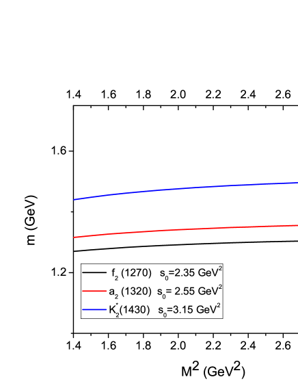
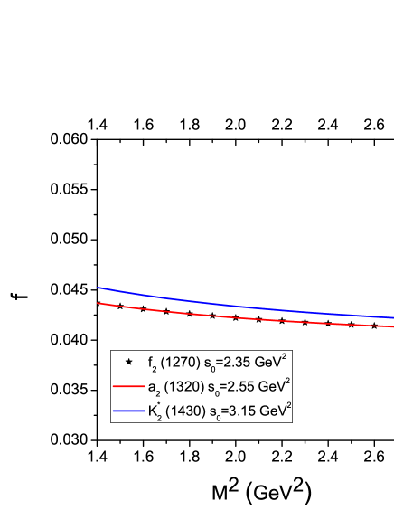
Figure 1: Variations of the masses and decay constants of the $K_{2}^{*}(1430)$, $f_{2}(1270)$ and $a_{2}(1320)$ mesons with respect to $M^{2}$ at fixed values of the continuum threshold and at zero temperature.

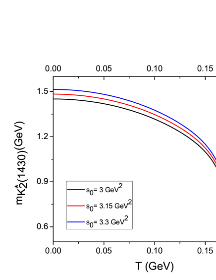
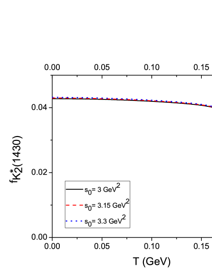
Figure 2: Temperature dependence of the mass and decay constant of the $K_{2}^{*}(1430)$ meson.

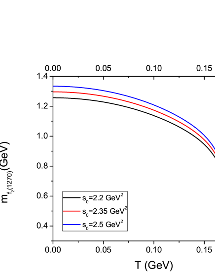
Figure 3: Temperature dependence of the mass and decay constant of the $f_{2}(1270)$ meson.

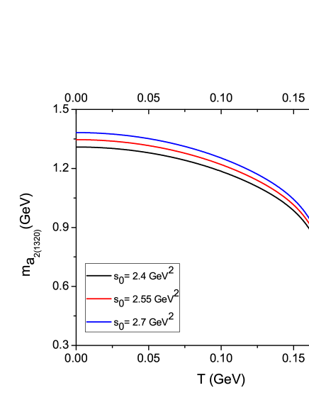
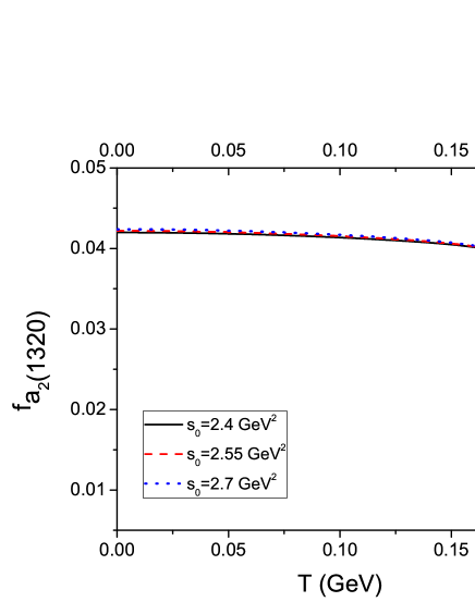
Figure 4: Temperature dependence of the mass and decay constant of the $a_{2}(1320)$ meson.

Now, we proceed to discuss how the physical quantities under consideration behave in terms of temperature in the working regions of the auxiliary parameters $M^{2}$ and $s_{0}$. For this aim, we present the dependence of the masses and decay constants on temperature at $M^{2}=2.2~{}GeV^{2}$ in figures 2, 3 and 4. Note that, we plot these figures up to the temperature that the temperature-dependent continuum threshold vanishes, i.e., $T\simeq 183~{}MeV$. From these figures, we see that the masses and decay constants diminish by increasing the temperature. Near to the temperature $T\simeq 183~{}MeV$, the decay constants of the $f_{2}(1270)$, $a_{2}(1320)$ and $K_{2}^{*}(1430)$ decrease with amount of $81\%$, $70\%$ and $85\%$ compared to their vacuum values, respectively. While, the masses decrease about $70\%$, $72\%$ and $60\%$ for $f_{2}(1270)$, $a_{2}(1320)$ and $K_{2}^{*}(1430)$ states, respectively.

$$\begin{array}[]{|c|c|c|c|c|c|c|c|}\hline\cr\hline\cr&\mbox{Present\,\,\,Work}&\mbox{Experiment}&\mbox{Vacuum\,\,Sum\,\,Rules}\,\,\cite[cite]{[\@@bibref{}{Aliev,Aliev2}{}{}]}\\ &&\cite[cite]{[\@@bibref{}{J. Beringer}{}{}]}&\mbox{Relativistic\,\, Quark \,\,Model}\,\,\cite[cite]{[\@@bibref{}{Ebert}{}{}]}\\ \hline\cr\mbox{$m_{K_{2}^{*}(1430)}$(GeV)}&1.48\pm 0.12&1.4256\pm 0.0015&1.44\pm 0.10~{}~{}~{}\cite[cite]{[\@@bibref{}{Aliev2}{}{}]},~{}~{}~{}1.424~{}~{}~{}\cite[cite]{[\@@bibref{}{Ebert}{}{}]}\\ \hline\cr\mbox{ $f_{K_{2}^{*}(1430)}$}&0.043\pm 0.002&-&0.050\pm 0.002~{}~{}\cite[cite]{[\@@bibref{}{Aliev2}{}{}]}\\ \hline\cr\mbox{$m_{f_{2}(1270)}$(GeV)}&1.30\pm 0.08&1.2751\pm 0.0012&1.25~{}~{}~{}~{}~{}\cite[cite]{[\@@bibref{}{Aliev}{}{}]}\\ \hline\cr\mbox{ $f_{f_{2}(1270)}$}&0.042\pm 0.002&-&0.040~{}~{}~{}~{}~{}\cite[cite]{[\@@bibref{}{Aliev}{}{}]}\\ \hline\cr\mbox{$m_{a_{2}(1320)}$(GeV)}&1.35\pm 0.11&1.3183\pm 0.0006&1.25~{}~{}~{}~{}~{}\cite[cite]{[\@@bibref{}{Aliev}{}{}]}\\ \hline\cr\mbox{ $f_{a_{2}(1320)}$}&0.042\pm 0.002&-&-\\ \hline\cr\hline\cr\end{array}$$

Table 1: Values of the masses and decay constants of the $K_{2}^{*}$, $f_{2}$ and $a_{2}$ mesons at zero temperature.

Our final task is to compare the results of this work obtained at zero temperature with those of the vacuum sum rules as well as other existing theoretical predictions and experimental data. This comparison is made in table 1. From this table we see that the results on the masses and decay constants obtained at zero temperature are roughly consistent with existing experimental data as well as the vacuum sum rules and relativistic quark model predictions within the uncertainties. Our predictions on the decay constants of the light tensor mesons can be checked in future experiments. The results obtained in the present work can be used in theoretical determination of the electromagnetic properties of the light tensor mesons as well as their weak decay parameters and their strong couplings with other hadrons. Our results on the thermal behavior of the masses and decay constants can also be useful in analysis of the results of future heavy ion collision experiments.

4 Acknowledgment

This work has been supported in part by the Scientific and Technological Research Council of Turkey (TUBITAK) under the research projects 110T284 and 114F018.

5 Conflict of Interests

The authors declare that there is no conflict of interests regarding the publication of this article.

References

• [1] G. E. Brown and M. Rho, Phys. Rep. 269, 333 (1996).
• [2] M. A. Shifman, A. I. Vainshtein, V. I. Zakharov, Nucl. Phys. B147, 385 (1979).
• [3] M. A. Shifman, A. I. Vainshtein, V. I. Zakharov, Nucl. Phys. B147, 448 (1979).
• [4] A. I. Bochkarev, M. E. Shaposhnikov, Nucl. Phys. B268, 220 (1986).
• [5] T. Hatsuda, Y. Koike and S. H. Lee, Nucl. Phys. B394, 221 (1993).
• [6] S. Mallik, Phys. Lett. B416, 373 (1998).
• [7] E.V. Shuryak, Rev. Mod. Phys. 65, 1 (1993).
• [8] S. Mallik and S. Sarkar, Eur. Phys. J. C25, 445 (2002).
• [9] T. Waas, N. Kaiser, W. Weise, Phys. Lett. B365, 12 (1996).
• [10] L. Tolos, D. Cabrera and A. Ramos, Phys. Rev. C78, 045205 (2008).
• [11] E. V. Veliev, J. Phys. G35, 035004 (2008).
• [12] E. V. Veliev, K. Azizi, H. Sundu, N. Aksit, J. Phys. G39, 015002 (2012).
• [13] E. V. Veliev, G. Kaya, Eur. Phys. J. C63, 87 (2009).
• [14] F. Klingl, S. Kim, S. H. Lee, P. Morath and W. Weise, Phys. Rev. Lett. 82, 3396 (1999).
• [15] C. A. Dominguez, M. Loewe, J.C. Rojas, JHEP 08, 040 (2007).
• [16] C. A. Dominguez, M. Loewe, Phys. Lett. B233, 201 (1989).
• [17] E. V. Veliev, K. Azizi, H. Sundu, G. Kaya, A. Türkan, Eur. Phys. J. A47, 110 (2011).
• [18] K. Azizi, H. Sundu, A. Türkan and E. V. Veliev, J. Phys. G41, 035003 (2014).
• [19] T. M. Aliev, M. A. Shifman, Phys. Lett. B112, 401 (1982).
• [20] D. Ebert, R. N. Faustov and V. O. Galkin, Phys. Rev. D79, 114029 (2009).
• [21] T. M. Aliev, K. Azizi and V. Bashiry, J. Phys. G37, 025001 (2010).
• [22] Z. G. Wang, Z. C. Liu, X. H. Zhang, Eur. Phys. J. C64, 373 (2009).
• [23] J. Beringer et al. (Particle Data Group), Phys. Rev. D86, 010001 (2012).
• [24] B. L. Ioffe, Prog. Part. Nucl. Phys. 56, 232 (2006).
• [25] S. Narison, Phys. Lett. B605, 319 (2005).
• [26] A. Barducci, R. Casalbuoni, S. De Curtis, R. Gatto, G. Pettini, Phys. Rev. D46, 2203 (1992).
• [27] A. Ayala, A. Bashir, C. A. Dominguez, E. Gutierrez, M. Loewe, A. Raya, Phys. Rev. D84, 056004 (2011).
• [28] A. Bazavov et al., Phys. Rev. D80, 014504 (2009).
• [29] M. Cheng et al., Phys. Rev. D81, 054504 (2010).