Distributed Methods for High-dimensional and Large-scale Tensor Factorization

Abstract

Given a high-dimensional large-scale tensor, how can we decompose it into latent factors? Can we process it on commodity computers with limited memory? These questions are closely related to recommender systems, which have modeled rating data not as a matrix but as a tensor to utilize contextual information such as time and location. This increase in the dimension requires tensor factorization methods scalable with both the dimension and size of a tensor. In this paper, we propose two distributed tensor factorization methods, SALS and CDTF. Both methods are scalable with all aspects of data, and they show an interesting trade-off between convergence speed and memory requirements. SALS updates a subset of the columns of a factor matrix at a time, and CDTF, a special case of SALS, updates one column at a time. In our experiments, only our methods factorize a 5-dimensional tensor with 1 billion observable entries, 10M mode length, and 1K rank, while all other state-of-the-art methods fail. Moreover, our methods require several orders of magnitude less memory than our competitors. We implement our methods on MapReduce with two widely-applicable optimization techniques: local disk caching and greedy row assignment. They speed up our methods up to 98.2$\times$ and also the competitors up to 5.9$\times$.

I Introduction and Related Work

Recommendation problems can be viewed as completing a partially observable user-item matrix whose entries are ratings. Matrix factorization (MF), which decomposes the input matrix into a user factor matrix and an item factor matrix such that their multiplication approximates the input matrix, is one of the most widely-used methods for matrix completion [chen2011linear, koren2009matrix, zhou2008large]. To handle web-scale data, efforts were made to find distributed ways for MF, including ALS [zhou2008large], DSGD [gemulla2011large], and CCD++ [yu2013parallel].

On the other hand, there have been attempts to improve the accuracy of recommendation by using additional contextual information such as time and location. A straightforward way to utilize such extra factors is to model rating data as a partially observable tensor where additional dimensions correspond to the extra factors. Similar to the matrix completion, tensor factorization (TF), which decomposes the input tensor into multiple factor matrices and a core tensor, has been used for tensor completion [Karatzoglou:2010, nanopoulos2010musicbox, zheng2010collaborative].

TABLE I: Summary of scalability results. The factors which each method is scalable with are checked. Our proposed SALS and CDTF are the only methods scalable with all the factors.

	CDTF	SALS	ALS	PSGD	FlexiFaCT
Dimension	✓	✓	✓	✓
Observations	✓	✓	✓	✓	✓
Mode Length	✓	✓			✓
Rank	✓	✓			✓
Machines	✓	✓	✓

As the dimension of web-scale recommendation problems increases, a necessity for TF algorithms scalable with the dimension as well as the size of data has arisen. A promising way to find such algorithms is to extend distributed MF algorithms to higher dimensions. However, the scalability of existing methods including ALS [zhou2008large], PSGD [mcdonald2010distributed], and FlexiFaCT [beutel2014flexifact] is limited as summarized in Table I.

In this paper, we propose Subset Alternating Least Square (SALS) and Coordinate Descent for Tensor Factorization (CDTF), distributed tensor factorization methods scalable with all aspects of data. SALS updates a subset of the columns of a factor matrix at a time, and CDTF, a special case of SALS, updates one column at a time. These two methods have distinct advantages: SALS converges faster, and CDTF is more memory-efficient. Our methods can also be used in any applications handling large-scale partially observable tensors, including social network analysis [dunlavy2011temporal] and Web search [sun2005cubesvd].

TABLE II: Summary of distributed tensor factorization algorithms. The performance bottlenecks which prevent each algorithm from handling web-scale data are colored red. Only our proposed SALS and CDTF have no bottleneck. Communication complexity is measured by the number of parameters that each machine exchanges with the others. For simplicity, we assume that workload of each algorithm is equally distributed across machines, that the length of every mode is equal to $I$, and that $T_{in}$ of SALS and CDTF is set to one.

Algorithm	Computational complexity	Communication complexity	Memory requirements	Convergence speed
	(per iteration)	(per iteration)
CDTF	$O(|\Omega|N^{2}K/M)$	$O(NIK)$	$O(NI)$	Fast
SALS	$O(|\Omega|NK(N+C)/M+NIKC^{2}/M)$	$O(NIK)$	$O(NIC)$	Fastest
ALS [zhou2008large]	$O(|\Omega|NK(N+K)/M+NIK^{3}/M)$	$O(NIK)$	$O(NIK)$	Fastest
PSGD [mcdonald2010distributed]	$O(|\Omega|NK/M)$	$O(NIK)$	$O(NIK)$	Slow
FlexiFaCT [beutel2014flexifact]	$O(|\Omega|NK/M)$	$O(M^{N-2}NIK)$	$O(NIK/M)$	Fast

The main contributions of our study are as follows:

Algorithm. We propose SALS and CDTF, scalable tensor factorization algorithms. Their distributed versions are the only methods scalable with all the following factors: the dimension and size of data, the number of parameters, and the number of machines (Table I).

Analysis. We analyze our methods and the competitors in a general N-dimensional setting in the following aspects: computational complexity, communication complexity, memory requirements, and convergence speed (Table II).

Optimization. We implement our methods on MapReduce with two widely-applicable optimization techniques: local disk caching and greedy row assignment. They speed up not only our methods (up to 98.2$\times$) but also the competitors (up to 5.9$\times$) (Figure LABEL:fig:impl).

Experiment. We empirically confirm the superior scalability of our methods and their several orders of magnitude less memory requirements than the competitors. Only our methods analyze a 5-dimensional tensor with 1 billion observable entries, 10M mode length, and 1K rank, while all others fail (Figure LABEL:fig:data_scale_overall).

TABLE III: Table of symbols.

Symbol	Definition
$\boldsymbol{\mathscr{X}}$	input tensor $(\in\mathbb{R}^{I_{1}\times I_{2}...\times I_{N}})$
$x_{i_{1}...i_{N}}$	$(i_{1},...,i_{N})$th entry of $\boldsymbol{\mathscr{X}}$
$N$	dimension of $\boldsymbol{\mathscr{X}}$
$I_{n}$	length of the $n$th mode of $\boldsymbol{\mathscr{X}}$
$\mathbf{A}^{(n)}$	$n$th factor matrix $(\in\mathbb{R}^{I_{n}\times K})$
$a^{(n)}_{i_{n}k}$	$(i_{n},k)$th entry of $\mathbf{A}^{(n)}$
$K$	rank of $\boldsymbol{\mathscr{X}}$
$\Omega$	set of indices of observable entries of $\boldsymbol{\mathscr{X}}$
$\Omega^{(n)}_{i_{n}}$	subset of $\Omega$ whose $n$th mode’s index is equal to $i_{n}$
${}_{m}S_{n}$	set of rows of $\mathbf{A}^{(n)}$ assigned to machine $m$
$\boldsymbol{\mathscr{R}}$	residual tensor $(\in\mathbb{R}^{I_{1}\times I_{2}...\times I_{N}})$
$r_{i_{1}...i_{N}}$	$(i_{1},...,i_{N})$th entry of $\boldsymbol{\mathscr{R}}$
$M$	number of machines (reducers on MapReduce)
$T_{out}$	number of outer iterations
$T_{in}$	number of inner iterations
$\lambda$	regularization parameter
$C$	number of parameters updated at a time
$\eta_{0}$	initial learning rate

The binary codes of our methods and several datasets are available at http://kdmlab.org/sals. The rest of this paper is organized as follows. Section II presents preliminaries for tensor factorization and its distributed algorithms. Section III describes our proposed SALS and CDTF methods. Section IV presents the optimization techniques for them on MapReduce. After providing experimental results in Section LABEL:sec:experiment, we conclude in Section LABEL:sec:conclusion.

II Preliminaries: Tensor Factorization

In this section, we describe the preliminaries of tensor factorization and its distributed algorithms.

II-A Tensor and the Notations

Tensors are multi-dimensional arrays that generalize vectors ($1$-dimensional tensors) and matrices ($2$-dimensional tensors) to higher dimensions. Like rows and columns in a matrix, an $N$-dimensional tensor has $N$ modes whose lengths are denoted by $I_{1}$ through $I_{N}$, respectively. We denote tensors with variable dimension $N$ by boldface Euler script letters, e.g., $\boldsymbol{\mathscr{X}}$. Matrices and vectors are denoted by boldface capitals, e.g., $\mathbf{A}$, and boldface lowercases, e.g., $\mathbf{a}$, respectively. We denote the entry of a tensor by the symbolic name of the tensor with its indices in subscript. For example, the $(i_{1},i_{2})$th entry of $\mathbf{A}$ is denoted by $a_{i_{1}i_{2}}$, and the $(i_{1},...,i_{N})$th entry of $\boldsymbol{\mathscr{X}}$ is denoted by $x_{i_{1}...i_{N}}$. The $i_{1}$th row of $\mathbf{A}$ is denoted by $\mathbf{a}_{i_{1}*}$, and the $i_{2}$th column of $\mathbf{A}$ is denoted by $\mathbf{a}_{*i_{2}}$. Table III lists the symbols used in this paper.

II-B Tensor Factorization

There are several ways to define a tensor factorization. Our definition is based on the PARAFAC decomposition [kolda2009tensor], which is one of the most popular decomposition methods, and the nonzero squared loss with $L_{2}$ regularization, whose weighted form has been successfully used in many recommender systems [chen2011linear, koren2009matrix, zhou2008large].

Definition 1 (Tensor Factorization)

Given an $N$-dimensional tensor $\boldsymbol{\mathscr{X}}(\in\mathbb{R}^{I_{1}\times I_{2}...\times I_{N}})$ with observable entries $\{x_{i_{1}...i_{N}}|(i_{1},...,i_{N})\in\Omega\}$, the rank $K$ factorization of $\boldsymbol{\mathscr{X}}$ is to find factor matrices $\{\mathbf{A}^{(n)}\in\mathbb{R}^{I_{n}\times K}|1\leq n\leq N\}$ which minimize the following loss function:

$$L(\mathbf{A}^{(1)},...,\mathbf{A}^{(N)})=\\ \sum_{(i_{1},...,i_{N})\in\Omega}{\left(x_{i_{1}...i_{N}}-\sum_{k=1}^{K}\prod_{n=1}^{N}a^{(n)}_{i_{n}k}\right)^{2}}+\lambda\sum_{n=1}^{N}{{\|\mathbf{A}^{(n)}\|}_{F}^{2}}$$ (1)

Note that the loss function depends only on the observable entries. Each factor matrix $\mathbf{A}^{(n)}$ corresponds to the latent feature vectors of the objects that the $n$th mode of $\boldsymbol{\mathscr{X}}$ represents, and $\sum_{k=1}^{K}\prod_{n=1}^{N}a^{(n)}_{i_{n}k}$ corresponds to the interaction among the features.

II-C Distributed Methods for Tensor Factorization

In this section, we explain how widely-used distributed optimization methods are applied to tensor factorization. Their performances are summarized in Table II. Note that only our proposed CDTF and SALS methods, which will be described in Sections III and IV, have no bottleneck in any aspects.

II-C1 Alternating Least Square (ALS)

Using ALS [zhou2008large], we update factor matrices one by one while keeping all other matrices fixed. When all other factor matrices are fixed, minimizing (1) is analytically solvable in terms of the updated matrix, which can be updated row by row due to the independence between rows. The update rule for each row of $\mathbf{A}^{(n)}$ is as follows:

$$[a^{(n)}_{i_{n}1},...,a^{(n)}_{i_{n}K}]^{T} \leftarrow\underset{[a^{(n)}_{i_{n}1},...,a^{(n)}_{i_{n}K}]^{T}}{\operatorname{arg}\,\operatorname{min}}\;{L(\mathbf{A}^{(1)},...,\mathbf{A}^{(N)})}$$

$$=(\mathbf{B}^{(n)}_{i_{n}}+\lambda\mathbf{I}_{K})^{-1}\mathbf{c}^{(n)}_{i_{n}}$$ (2)

where the $(k_{1},k_{2})$th entry of $\mathbf{B}^{(n)}_{i_{n}}(\in\mathbb{R}^{K\times K})$ is

$$\sum_{(i_{1},...,i_{N})\in\Omega^{(n)}_{i_{n}}}\left(\prod_{l\neq n}a^{(l)}_{i_{l}k_{1}}\prod_{l\neq n}a^{(l)}_{i_{l}k_{2}}\right),$$

the $k$th entry of $\mathbf{c}^{(n)}_{i_{n}}(\in\mathbb{R}^{K})$ is

$$\sum_{(i_{1},...,i_{N})\in\Omega^{(n)}_{i_{n}}}\left(x_{i_{1}...i_{N}}\prod_{l\neq n}a^{(l)}_{i_{l}k}\right),$$

and $\mathbf{I}_{K}$ is the $K$ by $K$ identity matrix. $\Omega^{(n)}_{i_{n}}$ denotes the subset of $\Omega$ whose $n$th mode’s index is $i_{n}$. This update rule can be proven as in Theorem 1 in Section III-A since ALS is a special case of SALS. Updating a row, $\mathbf{a}^{(n)}_{i_{n}*}$ for example, using (2) takes $O(|\Omega_{i_{n}}|K(N+K)+K^{3})$, which consists of $O(|\Omega^{(n)}_{i_{n}}|NK)$ to calculate $\prod_{l\neq n}a^{(l)}_{i_{l}1}$ through $\prod_{l\neq n}a^{(l)}_{i_{l}K}$ for all the entries in $\Omega^{(n)}_{i_{n}}$, $O(|\Omega^{(n)}_{i_{n}}|K^{2})$ to build $\mathbf{B}_{i_{n}}^{(n)}$, $O(|\Omega^{(n)}_{i_{n}}|K)$ to build $\mathbf{c}^{(n)}_{i_{n}}$, and $O(K^{3})$ to invert $\mathbf{B}_{i_{n}}^{(n)}$. Thus, updating every row of every factor matrix once, which corresponds to a full ALS iteration, takes $O(|\Omega|NK(N+K)+K^{3}\sum_{n=1}^{N}I_{n})$.

In distributed environments, updating each factor matrix can be parallelized without affecting the correctness of ALS by distributing the rows of the factor matrix across machines and updating them simultaneously. The parameters updated by each machine are broadcast to all other machines. The number of parameters each machine exchanges with the others is $O(KI_{n})$ for each factor matrix $\mathbf{A}^{(n)}$ and $O(K\sum_{n=1}^{N}I_{n})$ per iteration. The memory requirements of ALS, however, cannot be distributed. Since the update rule (2) possibly depends on any entry of any fixed factor matrix, every machine is required to load all the fixed matrices into its memory. This high memory requirements of ALS, $O(K\sum_{n=1}^{N}I_{n})$ memory space per machine, have been noted as a scalability bottleneck even in matrix factorization [gemulla2011large, yu2013parallel].

II-C2 Parallelized Stochastic Gradient Descent (PSGD)

PSGD [mcdonald2010distributed] is a distributed algorithm based on stochastic gradient descent (SGD). In PSGD, the observable entries of $\boldsymbol{\mathscr{X}}$ are randomly divided into $M$ machines which run SGD independently using the assigned entries. The updated parameters are averaged after each iteration. For each observable entry $x_{i_{1}...i_{N}}$, $a^{(n)}_{i_{n}k}$ for all $n$ and $k$, whose number is $NK$, are updated at once by the following rule :

$${a}^{(n)}_{i_{n}k}\leftarrow a^{(n)}_{i_{n}k}-2\eta\left(\frac{\lambda a^{(n)}_{i_{n}k}}{|\Omega^{(n)}_{i_{n}}|}-r_{i_{1}...i_{N}}\left(\prod_{l\neq n}{a^{(l)}_{i_{l}k}}\right)\right)$$ (3)

where $r_{i_{1}...i_{N}}=x_{i_{1}...i_{N}}-\sum_{s=1}^{K}\prod_{l=1}^{N}{a^{(l)}_{i_{l}s}}$. It takes $O(NK)$ to calculate $r_{i_{1}...i_{N}}$ and $\prod_{l=1}^{N}{a^{(l)}_{i_{l}k}}$ for all $k$. Once they are calculated, since $\prod_{l\neq n}{a^{(l)}_{i_{l}k}}$ can be calculated as $\left(\prod_{l=1}^{N}{a^{(l)}_{i_{l}k}}\right)/a^{(n)}_{i_{n}k}$, calculating (3) takes $O(1)$, and thus updating all the $NK$ parameters takes $O(NK)$. If we assume that $\boldsymbol{\mathscr{X}}$ entries are equally distributed across machines, the computational complexity per iteration is $O(|\Omega|NK/M)$. Averaging parameters can also be distributed, and in the process, $O(K\sum_{n=1}^{N}I_{n})$ parameters are exchanged by each machine. Like ALS, the memory requirements of PSGD cannot be distributed, i.e., all the machines are required to load all the factor matrices into their memory. $O(K\sum_{n=1}^{N}I_{n})$ memory space is required per machine. Moreover, PSGD tends to converge slowly due to the non-identifiability of (1) [gemulla2011large].

II-C3 Flexible Factorization of Coupled Tensors (FlexiFaCT)

FlexiFaCT [beutel2014flexifact] is another SGD-based algorithm that remedies the high memory requirements and slow convergence of PSGD. FlexiFaCT divides $\boldsymbol{\mathscr{X}}$ into $M^{N}$ blocks. Each $M$ disjoint blocks that do not share common fibers (rows in a general $n$th mode) compose a stratum. FlexiFaCT processes $\boldsymbol{\mathscr{X}}$ one stratum at a time in which the $M$ blocks composing a stratum are distributed across machines and processed independently. The update rule is the same as (3), and the computational complexity per iteration is $O(|\Omega|NK/M)$ as in PSGD. However, contrary to PSGD, averaging is unnecessary because a set of parameters updated by each machine are disjoint with those updated by the other machines. In addition, the memory requirements of FlexiFaCT are distributed among the machines. Each machine only needs to load the parameters related to the block it processes, whose number is $(K\sum_{n=1}^{N}I_{n})/M$, into its memory at a time. However, FlexiFaCT suffers from high communication cost. After processing one stratum, each machine sends the updated parameters to the machine which updates them using the next stratum. Each machine exchanges at most $(K\sum_{n=2}^{N}I_{n})/M$ parameters per stratum and $M^{N-2}K\sum_{n=2}^{N}I_{n}$ per iteration where $M^{N-1}$ is the number of strata. Thus, the communication cost increases exponentially with the dimension of $\boldsymbol{\mathscr{X}}$ and polynomially with the number of machines.

III Proposed methods

In this section, we propose Subset Alternating Least Square (SALS) and Coordinate Descent for Tensor Factorization (CDTF). They are scalable algorithms for tensor factorization, which is essentially an optimization problem whose loss function is (1) and parameters are the entries of factor matrices, $\mathbf{A}^{(1)}$ through $\mathbf{A}^{(N)}$. Figure 1 depicts the difference among CDTF, SALS, and ALS. Unlike ALS, which updates each $K$ columns of factor matrices row by row, SALS updates each $C$ $(1\leq C\leq K)$ columns row by row, and CDTF updates each column entry by entry. CDTF can be seen as an extension of CCD++ [yu2013parallel] to higher dimensions. Since SALS contains CDTF ($C=1$) as well as ALS ($T_{in}=1,C=K$) as a special case, we focus on SALS then explain additional optimization schemes for CDTF.

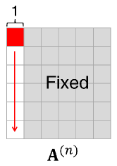
(a) CDTF

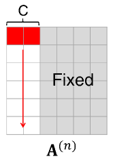
(b) SALS

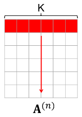
(c) ALS

Figure 1: Update rules of CDTF, SALS, and ALS. CDTF updates each column of factor matrices entry by entry, SALS updates each $C$ $(1\leq C\leq K)$ columns row by row, and ALS updates each $K$ columns row by row.

III-A Update Rule and Update Sequence

Input :  $\boldsymbol{\mathscr{X}}$, $K$, $\lambda$

Output :  $\mathbf{A}^{(n)}$ for all $n$

initialize $\boldsymbol{\mathscr{R}}$ and $\mathbf{A}^{(n)}$ for all $n$

for outer iter = 1..$T_{out}$ do  for split iter = 1..$\lceil\frac{K}{C}\rceil$ do  choose $k_{1},...,k_{C}$ (from columns not updated yet)

compute $\boldsymbol{\mathscr{\hat{R}}}$

for inner iter = 1..$T_{in}$ do  for n = 1..$N$ do  for $i_{n}$ = 1..$I_{n}$ do  update $a^{(n)}_{i_{n}k_{1}},...,a^{(n)}_{i_{n}k_{C}}$ using (4)

      update $\boldsymbol{\mathscr{R}}$ using (5)

   

Algorithm 1 Serial version of SALS

5

5

5

5

5

Algorithm 1 describes the procedure of SALS. $\boldsymbol{\mathscr{R}}$ denotes the residual tensor where $r_{i_{1}...i_{N}}=x_{i_{1}...i_{N}}-\sum_{k=1}^{K}\prod_{n=1}^{N}{a^{(n)}_{i_{n}k}}$. We initialize the entries of $\mathbf{A}^{(1)}$ to zeros and those of all other factor matrices to random values so that the initial value of $\boldsymbol{\mathscr{R}}$ is equal to $\boldsymbol{\mathscr{X}}$ (line 1). In every iteration (line 1), SALS repeats choosing $C$ columns, $k_{1}$ through $k_{C}$, randomly without replacement (line 1) and updating them while keeping the other columns fixed, which is equivalent to the rank $C$ factorization of $\boldsymbol{\mathscr{\hat{R}}}$ where $\hat{r}_{i_{1}...i_{N}}=r_{i_{1}...i_{N}}+\sum_{c=1}^{C}\prod_{n=1}^{N}a^{(n)}_{i_{n}k_{c}}$. Once $\boldsymbol{\mathscr{\hat{R}}}$ is computed (line 1), updating $C$ columns of factor matrices matrix by matrix (line 1) is repeated $T_{in}$ times (line 1). For each factor matrix, since its rows are independent of each other in minimizing (1) when the other factor matrices are fixed, the entries are updated row by row (line 1) as follows:

$$[a^{(n)}_{i_{n}k_{1}},...,a^{(n)}_{i_{n}k_{C}}]^{T}\leftarrow \underset{[a^{(n)}_{i_{n}k_{1}},...,a^{(n)}_{i_{n}k_{C}}]^{T}}{\operatorname{arg}\,\operatorname{min}}\;{L(\mathbf{A}^{(1)},...,\mathbf{A}^{(N)})}$$

$$=(\mathbf{B}^{(n)}_{i_{n}}+\lambda\mathbf{I}_{C})^{-1}\mathbf{c}^{(n)}_{i_{n}},$$ (4)

where the $(c_{1},c_{2})$th entry of $\mathbf{B}^{(n)}_{i_{n}}(\in\mathbb{R}^{C\times C})$ is

$$\sum_{(i_{1},...,i_{N})\in\Omega^{(n)}_{i_{n}}}\left(\prod_{l\neq n}a^{(l)}_{i_{l}k_{c_{1}}}\prod_{l\neq n}a^{(l)}_{i_{l}k_{c_{2}}}\right),$$

the $c$th entry of $\mathbf{c}^{(n)}_{i_{n}}(\in\mathbb{R}^{C})$ is

$$\sum_{(i_{1},...,i_{N})\in\Omega^{(n)}_{i_{n}}}\left(\hat{r}_{i_{1}...i_{N}}\prod_{l\neq n}a^{(l)}_{i_{l}k_{c}}\right),$$

and $\mathbf{I}_{C}$ is the $C$ by $C$ identity matrix. $\Omega^{(n)}_{i_{n}}$ denotes the subset of $\Omega$ whose $n$th mode’s index is $i_{n}$. The proof of this update rule is as follows:

Theorem 1

$$\underset{[a^{(n)}_{i_{n}k_{1}},...,a^{(n)}_{i_{n}k_{C}}]^{T}}{\operatorname{arg}\,\operatorname{min}}\;{L(\mathbf{A}^{(1)},...,\mathbf{A}^{(N)})}=(\mathbf{B}^{(n)}_{i_{n}}+\lambda\mathbf{I}_{C})^{-1}\mathbf{c}^{(n)}_{i_{n}}$$

Proof:

$$\frac{\partial L}{\partial a^{(n)}_{i_{n}k_{c}}}=0,\forall c,1\leq c\leq C$$

$$\Leftrightarrow\sum_{(i_{1},...,i_{N})\in\Omega^{n}_{i_{n}}}{\left(\left(\sum_{s=1}^{C}\prod_{l=1}^{N}a^{(l)}_{i_{l}k_{s}}-\hat{r}_{i_{1}...i_{N}}\right)\prod_{l\neq n}a^{(l)}_{i_{l}k_{c}}\right)}+\lambda a^{(n)}_{i_{n}k_{c}}$$

$$\;\;\;=0,\forall c$$

$$\Leftrightarrow\sum_{(i_{1},...,i_{N})\in\Omega^{n}_{i_{n}}}{\left(\sum_{s=1}^{C}\left(a^{(n)}_{i_{n}k_{s}}\prod_{l\neq n}a^{(l)}_{i_{l}k_{s}}\right)\prod_{l\neq n}a^{(l)}_{i_{l}k_{c}}\right)}+\lambda a^{(n)}_{i_{n}k_{c}}$$

$$\;\;\;=\sum_{(i_{1},...,i_{N})\in\Omega^{n}_{i_{n}}}\left(\hat{r}_{i_{1}...i_{N}}\prod_{l\neq n}a^{(l)}_{i_{l}k_{c}}\right),\forall c$$

$$\Leftrightarrow(\mathbf{B}^{(n)}_{i_{n}}+\lambda\mathbf{I}_{c})[a^{(n)}_{i_{n}k_{1}},...,a^{(n)}_{i_{n}k_{C}}]^{T}=\mathbf{c}^{(n)}_{i_{n}}$$

∎

Since $\mathbf{B}^{(n)}_{i_{n}}$ is symmetric, instead of computing its inverse, the Cholesky decomposition can be used. After this rank $C$ factorization, the entries of $\boldsymbol{\mathscr{R}}$ are updated by the following rule (line 1):

$$\small r_{i_{1}...i_{N}}\leftarrow\hat{r}_{i_{1}...i_{N}}-\sum_{c=1}^{C}\prod_{n=1}^{N}a^{(n)}_{i_{n}k_{c}}.$$ (5)

CDTF is a special case of SALS where $C$ is set to one. In CDTF, instead of computing $\boldsymbol{\mathscr{\hat{R}}}$ before rank one factorization, the entries of $\boldsymbol{\mathscr{\hat{R}}}$ can be computed while computing (4) and (5). This can result in better performance on a disk-based system like MapReduce by reducing disk I/O operations. Moreover, instead of randomly changing the order by which columns are updated at each iteration, fixing the order speeds up the convergence of CDTF in our experiments.

III-B Complexity Analysis

Theorem 2

The computational complexity of Algorithm 1 is $O(T_{out}|\Omega|NT_{in}K(N+C)+T_{out}T_{in}KC^{2}\sum_{n=1}^{N}I_{n})$.

Proof:

Computing $\boldsymbol{\mathscr{\hat{R}}}$ (line 1) and updating $\boldsymbol{\mathscr{R}}$ (line 1) take $O(|\Omega|NC)$. Updating $C$ parameters (line 1) takes $O(|\Omega^{(n)}_{i_{n}}|C(C+N)+C^{3})$, which consists of $O(|\Omega^{(n)}_{i_{n}}|NC)$ to calculate $\prod_{l\neq n}a^{(l)}_{i_{l}k_{1}}$ through $\prod_{l\neq n}a^{(l)}_{i_{l}k_{C}}$ for all the entries in $|\Omega|^{(n)}_{i_{n}}$, $O(|\Omega^{(n)}_{i_{n}}|C^{2})$ to build $\mathbf{B}_{i_{n}}^{(n)}$, $O(|\Omega^{(n)}_{i_{n}}|C)$ to build $\mathbf{c}^{(n)}_{i_{n}}$, and $O(C^{3})$ to invert $\mathbf{B}_{i_{n}}^{(n)}$. Thus, updating all the entries in $C$ columns (lines 1 through 1) takes $O(|\Omega|C(C+N)+I_{n}C^{3})$, and the rank $C$ factorization (lines 1 through 1) takes $O(|\Omega|NC(N+C)+C^{3}\sum_{n=1}^{N}I_{n})$. As a result, an outer iteration, which repeats the rank $C$ factorization $T_{in}K/C$ times and both $\boldsymbol{\mathscr{\hat{R}}}$ computation and $\boldsymbol{\mathscr{R}}$ update $K/C$ times, takes $O(|\Omega|NT_{in}K(N+C)+T_{in}KC^{2}\sum_{n=1}^{N}I_{n})+O(|\Omega|NK)$, where the second term is dominated. ∎

Theorem 3

The memory requirement of Algorithm 1 is $O(C\sum_{n=1}^{N}I_{n})$.

Proof:

Since $\boldsymbol{\mathscr{\hat{R}}}$ computation (line 1), rank $C$ factorization (lines 1 through 1), and $\boldsymbol{\mathscr{R}}$ update (line 1) all depend only on the $C$ columns of the factor matrices, the number of whose entries is $C\sum_{n=1}^{N}I_{n}$, the other $(K-C)$ columns do not need to be loaded into memory. Thus, the columns of the factor matrices can be loaded by turns depending on $(k_{1},...,k_{C})$ values. Moreover, updating $C$ columns (lines 1 through 1) can be processed by streaming the entries of $\boldsymbol{\mathscr{\hat{R}}}$ from disk and processing them one by one instead of loading them all at once because the entries of $\mathbf{B}^{(n)}_{i_{n}}$ and $\mathbf{c}^{(n)}_{i_{n}}$ in (4) are the sum of the values calculated independently from each $\boldsymbol{\mathscr{\hat{R}}}$ entry. Likewise, $\boldsymbol{\mathscr{\hat{R}}}$ computation and $\boldsymbol{\mathscr{R}}$ update can also be processed by streaming $\boldsymbol{\mathscr{R}}$ and $\boldsymbol{\mathscr{\hat{R}}}$, respectively. ∎

III-C Parallelization in Distributed Environments

In this section, we describe how to parallelize SALS in distributed environments such as MapReduce where machines do not share memory. Algorithm 2 depicts the distributed version of SALS.

Input :  $\boldsymbol{\mathscr{X}}$, $K$, $\lambda$, ${}_{m}S_{n}$ for all $m$ and $n$

Output :  $\mathbf{A}^{(n)}$ for all $n$

distribute the ${}_{m}\Omega$ entries of $\boldsymbol{\mathscr{X}}$ to each machine $m$

Parallel (P): initialize the ${}_{m}\Omega$ entries of $\boldsymbol{\mathscr{R}}$

P: initialize $\mathbf{A}^{(n)}$ for all $n$

for outer iter = 1..$T_{out}$ do  for split iter = 1..$\lceil\frac{K}{C}\rceil$ do  choose $k_{1},...,k_{C}$ (from columns not updated yet)

P: compute ${}_{m}\Omega$ entries of $\boldsymbol{\mathscr{\hat{R}}}$

for inner iter = 1..$T_{in}$ do  for n = 1..$N$ do  P: update $\{a^{(n)}_{i_{n}k_{c}}|i_{n}\in{}_{m}S_{n},1\leq c\leq C\}$ using (4)

P: broadcast $\{a^{(n)}_{i_{n}k_{c}}|i_{n}\in{}_{m}S_{n},1\leq c\leq C\}$

    P: update the ${}_{m}\Omega$ entries of $\boldsymbol{\mathscr{R}}$ using (5)

   

Algorithm 2 Distributed version of SALS

8

8

8

8

8

8

8

8

Since update rule (4) for each row (C parameters) of a factor matrix does not depend on the other rows in the matrix, rows in a factor matrix can be distributed across machines and updated simultaneously without affecting the correctness of SALS. Each machine $m$ updates ${}_{m}S_{n}$ rows of $\mathbf{A}^{(n)}$ (line 2), and for this, the ${}_{m}\Omega=\bigcup_{n=1}^{N}\left(\bigcup_{i_{n}\in{}_{m}S_{n}}\Omega^{(n)}_{i_{n}}\right)$ entries of $\boldsymbol{\mathscr{X}}$ are distributed to machine $m$ in the first stage of the algorithm (line 2). Figure 2 shows an example of work and data distribution in SALS.

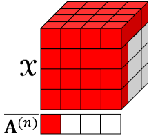
(a) Machine 1

(b) Machine 2

(c) Machine 3

(d) Machine 4

Figure 2: Work and data distribution of SALS in distributed environments when an input tensor is a three-dimensional tensor and the number of machines is four. We assume that the rows of the factor matrices are assigned to the machines sequentially. The colored region of $\overline{\mathbf{A}^{(n)}}$ (the transpose of $\mathbf{A}^{(n)}$) in each sub-figure corresponds to the parameters updated by each machine, resp., and that of $\boldsymbol{\mathscr{X}}$ corresponds to the data distributed to each machine.

After the update, parameters updated by each machine are broadcast to all other machines (line 2). Each machine $m$ broadcasts $C|{}_{m}S_{n}|$ parameters and receives $C(I_{n}-|{}_{m}S_{n}|)$ parameters from the other machines after each update. The total number of parameters each machine exchanges with the other machines is $KT_{in}\sum_{n=1}^{N}I_{n}$ per outer iteration.

The running time of parallel steps in Algorithm 2 depends on the longest running time among all machines. Specifically, the running time of lines 2, 2, and 2 is proportional to $\max_{m}|{}_{m}\Omega^{(n)}|$ where ${}_{m}\Omega^{(n)}=\bigcup_{i_{n}\in{}_{m}S_{n}}\Omega^{(n)}_{i_{n}}$, and that of line 2 is proportional to $\max_{m}|{}_{m}S_{n}|$. Therefore, it is necessary to assign the rows of the factor matrices to the machines (i.e., to decide ${}_{m}S_{n}$) so that $|{}_{m}\Omega^{(n)}|$ and $|{}_{m}S_{n}|$ are even among all the machines. The greedy assignment algorithm described in Algorithm 3 aims to minimize $\max_{m}|{}_{m}\Omega^{(n)}|$ under the condition that $\max_{m}|{}_{m}S_{n}|$ is minimized (i.e., $|{}_{m}S_{n}|=I_{n}/M$ for all $n$ where $M$ is the number of machines). For each factor matrix $\mathbf{A}^{(n)}$, we sort its rows in the decreasing order of $|\Omega^{(n)}_{i_{n}}|$ and assign the rows one by one to the machine $m$ which satisfies $|{}_{m}S_{n}|<\lceil I_{n}/M\rceil$ and has the smallest $|{}_{m}\Omega^{(n)}|$ currently. The effects of this greedy row assignment on actual running times are analyzed in Section LABEL:sec:exp:optimization.

Input :  $\boldsymbol{\mathscr{X}}$, $M$

Output :  ${}_{m}S_{n}$ for all $m$ and $n$

initialize $|{}_{m}\Omega|$ to $0$ for all $m$

for n = 1..$N$ do  initialize ${}_{m}S_{n}$ to $\emptyset$ for all $m$

initialize $|{}_{m}\Omega^{(n)}|$ to $0$ for all $m$

calculate $|\Omega^{(n)}_{i_{n}}|$ for all $i_{n}$

foreach $i_{n}$ (in decreasing order of $|\Omega^{(n)}_{i_{n}}|$) do  find $m$ with $|{}_{m}S_{n}|<\lceil\frac{I_{n}}{M}\rceil$ and the smallest $|{}_{m}\Omega^{(n)}|$

(in case of a tie, choose the machine with smaller $|{}_{m}S_{n}|$, and if still a tie, choose the one with smaller $|{}_{m}\Omega|$)

add $i_{n}$ to ${}_{m}S_{n}$

add $|\Omega^{(n)}_{i_{n}}|$ to $|{}_{m}\Omega^{(n)}|$ and $|{}_{m}\Omega|$

   

Algorithm 3 Greedy row assignment in SALS

9

9

9

9

9

9

9

9

9

IV Optimization on MapReduce

In this section, we describe two optimization techniques used to implement SALS and CDTF on MapReduce, which is one of the most widely-used distributed platforms.

Given : $n$, $k_{c}$ for all $c$, ${}_{m}S_{n}$ for all $m$, $\mathbf{a}^{(l)}_{*k_{c}}$ for all $l$ and $c$

Input : $\boldsymbol{\mathscr{\hat{R}}}$

Output : updated $a^{(n)}_{*k_{c}}$ for all $c$

Map(Key k, Value v)

begin  $((i_{1},...,i_{N})$, $\hat{r}_{i_{1}...i_{N}})$ $\leftarrow$ v

find $m$ where $i_{n}\in{}_{m}S_{n}$

emit $<(m,i_{n}),((i_{1},...,i_{N}),\hat{r}_{i_{1}...i_{N}})>$ end

Partitioner(Key k, Value v)

begin  $(m,i_{n})$ $\leftarrow$ k

assign $<k,v>$ to machine $m$ end

Reduce(Key k, Value v[1..r])

begin  $(m,i_{n})$ $\leftarrow$ k

$\Omega^{(n)}_{i_{n}}$ entries of $\boldsymbol{\mathscr{\hat{R}}}$ $\leftarrow$ v

update and emit $a^{(n)}_{i_{n}k_{c}}$ for all $c$ end

Algorithm 4 Parameter update in SALS without local disk caching

11

11

11

11

11

11

11

11

11

11

11

Given : $k_{c}$ for all $c$, ${}_{m}S_{1}$ for all $m$, $\mathbf{a}^{(l)}_{*k_{c}}$ for all $l$ and $c$

Input : $\boldsymbol{\mathscr{\hat{R}}}$

Output : updated $\boldsymbol{\mathscr{R}}$

Map(Key k, Value v)

begin  $((i_{1},...,i_{N})$, $\hat{r}_{i_{1}...i_{N}})$ $\leftarrow$ v

find $m$ where $i_{1}\in{}_{m}S_{1}$

emit $<m,((i_{1},...,i_{N}),\hat{r}_{i_{1}...i_{N}})>$ end

Partitioner(Key k, Value v)

begin  $m$ $\leftarrow$ k

assign $<k,v>$ to machine $m$ end

Reduce(Key k, Value v[1..r])

begin  foreach $((i_{1},...,i_{N})$, $\hat{r}_{i_{1}...i_{N}})\in$ v[1…r] do  update $r_{i_{1}...i_{N}}$

emit $((i_{1},...,i_{N})$, $r_{i_{1}...i_{N}})$   end

Algorithm 5 $\boldsymbol{\mathscr{R}}$ update in SALS without local disk caching

10

10

10

10

10

10

10

10

10

10

Input :  $\boldsymbol{\mathscr{X}}$, ${}_{m}S_{n}$ for all $m$ and $n$

Output :  ${}_{m}\Omega^{(n)}$ entries of $\boldsymbol{\mathscr{R}}(=\boldsymbol{\mathscr{X}})$ for all $m$ and $n$

Map(Key k, Value v) ;

begin  $((i_{1},...,i_{N})$, $x_{i_{1}...i_{N}})$ $\leftarrow$ v

for n = 1,…,$N$ do  find $m$ where $i_{n}\in{}_{m}S_{n}$

emit $<(m,n),((i_{1},...,i_{N}),x_{i_{1}...i_{N}})>$   end

Partitioner(Key k, Value v) ;

begin  $(m,n)$ $\leftarrow$ k

assign $<k,v>$ to machine $m$ end

Reduce(Key k, Value v[1..r]) ;

begin  $(m,n)$ $\leftarrow$ k

open a file on the local disk to cache ${}_{m}\Omega^{(n)}$ entries of $\boldsymbol{\mathscr{R}}$

foreach $((i_{1},...,i_{N})$, $x_{i_{1}...i_{N}})\in$ v[1…r] do  write $((i_{1},...,i_{N})$, $x_{i_{1}...i_{N}})$ to the file

  end

Algorithm 6 Data distribution in SALS with local disk caching

12

12

12

12

12

12

12

12

12

12

12

12

IV-A Local Disk Caching

Typical MapReduce implementations of SALS and CDTF without local disk caching run each parallel step as a separate MapReduce job. Algorithms 4 and 5 describe the MapReduce implementation of parameter update (update of $a^{(n)}_{*k_{c}}$ for all $c$) and $\boldsymbol{\mathscr{R}}$ update, respectively. $\boldsymbol{\mathscr{\hat{R}}}$ computation can be implemented by the similar way with $\boldsymbol{\mathscr{R}}$ update. in this implementation, broadcasting updated parameters is unnecessary because reducers terminate after updating their assigned parameters. Instead, the updated parameters are saved in the distributed file system and are read at the next step (a separate job). Since SALS repeats both $\boldsymbol{\mathscr{R}}$ update and $\boldsymbol{\mathscr{\hat{R}}}$ computation $K/C$ times and parameter update $KT_{in}N/C$ times at every outer iteration, this implementation repeats distributing $\boldsymbol{\mathscr{R}}$ or $\boldsymbol{\mathscr{\hat{R}}}$ across machines (the mapper stage of Algorithms 4 and 5) $T_{out}K(T_{in}N+2)/C$ times, which is inefficient.

Our implementation reduces this inefficiency by caching data to local disk once they are distributed. In the SALS implementation with local disk caching, $\boldsymbol{\mathscr{X}}$ entries are distributed across machines and cached in the local disk during the map and reduce stages (Algorithm 6); and the rest part of SALS runs in the close stage (cleanup stage in Hadoop) using cached data. Our implementation streams the cached data from the local disk instead of distributing entire $\boldsymbol{\mathscr{R}}$ or $\boldsymbol{\mathscr{\hat{R}}}$ from the distributed file system when updating factor matrices. For example, ${}_{m}\Omega^{(n)}$ entries of $\boldsymbol{\mathscr{\hat{R}}}$ are streamed from the local disk when the columns of $\mathbf{A}^{(n)}$ are updated. The effect of this local disk caching on the actual running time is analyzed in Section LABEL:sec:exp:optimization.

IV-B Direct Communication

In MapReduce, it is generally assumed that reducers run independently and do not communicate directly with each other. However, we adapt the direct communication method using the distributed file system in [beutel2014flexifact] to broadcast parameters among reducers efficiently. The implementation of parameter broadcast in SALS (i.e., broadcast of $\mathbf{a}^{(n)}_{*k_{c}}$ for all $c$) based on this method is described in Algorithm 7 where ${}_{m}\mathbf{a}^{(n)}_{*k_{c}}$ denotes $\{a^{(n)}_{i_{n}k_{c}}|i_{n}\in{}_{m}S_{n}\}$.

Input : ${}_{m}\mathbf{a}^{(n)}_{*k_{c}}$ for all $c$ (parameters to broadcast)

Output :  $\mathbf{a}^{(n)}_{*k_{c}}$ for all c (parameters received from others)

begin  create a data file ${}_{m}A$ on the distributed file system (DFS)

write ${}_{m}\mathbf{a}^{(n)}_{*k}$ on the data file

create a dummy file ${}_{m}D$ on DFS

while not all data files were read do  get the list of dummy files from DFS

foreach ${}_{m^{\prime}}D$ in the list do  if ${}_{m^{\prime}}A$ were not read then  read ${}_{m^{\prime}}\mathbf{a}^{(n)}_{*k}$ from ${}_{m^{\prime}}A$

   

Algorithm 7 Parameter broadcast in SALS