On Succinct Representations of Binary Trees

Abstract

We observe that a standard transformation between ordinal trees (arbitrary rooted trees with ordered children) and binary trees leads to interesting succinct binary tree representations. There are four symmetric versions of these transformations. Via these transformations we get four succinct representations of $n$-node binary trees that use $2n+n/(\log n)^{O(1)}$ bits and support (among other operations) navigation, inorder numbering, one of pre- or post-order numbering, subtree size and lowest common ancestor (LCA) queries. The ability to support inorder numbering is crucial for the well-known range-minimum query (RMQ) problem on an array $A$ of $n$ ordered values. While this functionality, and more, is also supported in $O(1)$ time using $2n+o(n)$ bits by Davoodi et al.’s (Phil. Trans. Royal Soc. A 372 (2014)) extension of a representation by Farzan and Munro (Algorithmica 6 (2014)), their redundancy, or the $o(n)$ term, is much larger, and their approach may not be suitable for practical implementations.

One of these transformations is related to the Zaks’ sequence (S. Zaks, Theor. Comput. Sci. 10 (1980)) for encoding binary trees, and we thus provide the first succinct binary tree representation based on Zaks’ sequence. Another of these transformations is equivalent to Fischer and Heun’s (SIAM J. Comput. 40 (2011)) 2d-Min-Heap structure for this problem. Yet another variant allows an encoding of the Cartesian tree of $A$ to be constructed from $A$ using only $O(\sqrt{n}\log n)$ bits of working space.

1 Introduction

Binary trees are ubiquitous in computer science, and are integral to many applications that involve indexing very large text collections. In such applications, the space usage of the binary tree is an important consideration. While a standard representation of a binary tree node would use three pointers—to its left and right children, and to its parent—the space usage of this representation, which is $\Theta(n\log n)$ bits to store an $n$-node tree, is unacceptable in large-scale applications. A simple counting argument shows that the minimum space required to represent an $n$-node binary tree is $2n-O(\log n)$ bits in the worst case. A number of succinct representations of static binary trees have been developed that support a wide range of operations in $O(1)$ time, using only $2n+o(n)$ bits [15, 6].

However, succinct binary tree representations have limitations. A succinct binary tree representation can usually be divided into two parts: a tree encoding, which gives the structure of the tree, and takes close to $2n$ bits, and an index of $o(n)$ bits which is used to perform operations on the given tree encoding. It appears that the tree encoding constrains both the way nodes are numbered and the operations that can be supported in $O(1)$ time using a $o(n)$-bit index. For example, the earliest succinct binary tree representation was due to Jacobson [15], but this only supported a level-order numbering, and while it supported basic navigational operations such as moving to a parent, left child or right child in $O(1)$ time, it did not support operations such as lowest common ancestor (LCA) and reporting the size of the subtree rooted at a given node, in $O(1)$ time (indeed, it still remains unknown if there is a $o(n)$-bit index to support these operations in Jacobson’s encoding).

The importance of having a variety of node numberings and operations is illustrated by the range minimum query (RMQ) problem, defined as follows. Given an array $A[1..n]$ of totally ordered values, RMQ problem is to preprocess $A$ into a data structure to answer the query $\text{RMQ}(i,j)$: given two indexes $1\leq i\leq j\leq n$, return the index of the minimum value in $A[i..j]$. The aim is to minimize the query time, the space requirement of the data structure, as well as the time and space requirements of the preprocessing. This problem finds variety of applications including range searching [23], text indexing [1, 20], text compression [4], document retrieval [17, 21, 24], flowgraphs [11], and position-restricted pattern matching [14]. Since many of these applications deal with huge datasets, highly space-efficient solutions to the RMQ problem are of great interest.

A standard approach to solve the RMQ problem is via the Cartesian tree [25]. The Cartesian tree of $A$ is a binary tree obtained by labelling the root with the value $i$ where $A[i]$ is the smallest element in $A$. The left subtree of the root is the Cartesian tree of $A[1..i-1]$ and the right subtree of the root is the Cartesian tree of $A[i+1..n]$ (the Cartesian tree of an empty sub-array is the empty tree). As far as the RMQ problem is concerned, the key property of the Cartesian tree is that the answer to the query $\text{RMQ}(i,j)$ is the label of the node that is the lowest common ancestor (LCA) of the nodes labelled $i$ and $j$ in the Cartesian tree. Answering RMQs this way does not require access to $A$ at query time: this means that $A$ can be (and often is) discarded after pre-processing. Since Farzan and Munro [6] showed how to represent binary trees in $2n+o(n)$ bits and support LCA queries in $O(1)$ time, it would appear that there is a fast and highly space-efficient solution to the RMQ problem.

Unfortunately, this is not true. The difficulty is that the label of a node in the Cartesian tree (the index of the corresponding array element) is its rank in the inorder traversal of the Cartesian tree. Until recently, none of the known binary tree representations [15, 6, 7] was known to support inorder numbering. Indeed, the first $2n+o(n)$-bit and $O(1)$-time solution to the RMQ problem used an ordinal tree, or an arbitrary rooted, ordered tree, to answer RMQs [8].

Recently, Davoodi et al. [5] augmented the representation of [6] to support inorder numbering. However, Davoodi et al.’s result has some shortcomings. The $o(n)$ additive term—the redundancy—can be a significant overhead for practical values of $n$. Using the results of [18] (expanded upon in [22]), the redundancy of Jacobson’s binary tree representation, as well as Fischer and Heun’s RMQ solution, can be reduced to $n/(\log n)^{O(1)}$: this is not known to be true for the results of [6, 5]. Furthermore, there are several good practical implementations of ordinal trees [2, 13, 12], but the approach of [6, 5] is complex and needs significant work before its practical potential can even be evaluated. Finally, the results of [6, 5] do not focus on the construction space or time, while this is considered in [8].

Our Results.

We recall that there is a well-known transformation between binary trees and ordinal trees (in fact, there are four symmetric versions of this transformation). This allows us to represent a binary tree succinctly by transforming it into an ordinal tree, and then representing the ordinal tree succinctly. We note a few interesting properties of the resulting binary tree representations:

• The resulting binary tree representations support inorder numbering in addition to either postorder or preorder.

• The resulting binary tree representations support a number of operations including basic navigation, subtree size and LCA in $O(1)$ time; the latter implies in particular that they are suitable for the RMQ problem.

• The resulting binary tree representations use $2n+n/(\log n)^{O(1)}$ bits of space, and so have low redundancy.

• Since there are implementations of ordinal trees that are very fast in practice [2, 13, 12], we believe the resulting binary tree representations will perform well in practice.

• One of the binary tree representations, when applied to represent the Cartesian tree, gives the same data structure as the 2d-Min-Heap of Fischer and Heun [8].

• If one represents the ordinal tree using the BP encoding [19] then the resulting binary tree encoding is Zaks’ sequence [26]; we believe this to be the first succinct binary tree representation based on Zaks’ sequence sequence.

Finally, we also show in Section 3 that using these representations, we can make some improvements to the preprocessing phase of the RMQ problem. Specifically, we show that given an array $A$, a $2n+O(1)$-bit encoding of the tree structure of the Cartesian tree of $A$ can be created in linear time using only $O(\sqrt{n}\log n)$ bits of working space. This encoding can be augmented with additional data structures of size $o(n)$ bits, using only $o(n)$ bits of working space, thereby “improving” the result of [8] where $n+o(n)$ working space is used (the accounting of space is slightly different).

1.1 Preliminaries

Ordinal Tree Encodings.

We now discuss two encodings of ordinal trees. The first encoding is the natural balanced parenthesis (BP) encoding [15, 16]. The BP sequence of an ordinal tree is obtained by performing a depth-first traversal, and writing an opening parenthesis each time a node is visited, and a closing parenthesis immediately after all its descendants are visited. This gives a $2n$-bit encoding of an $n$-node ordinal tree as a sequence of balanced parentheses. The depth-first unary degree sequence (DFUDS) [3] is another encoding of an $n$-node ordinal tree as a sequence of balanced parentheses. This again visits the nodes in depth-first order (specifically, pre-order) and outputs the degree $d$ of each node—defined here as the number of children it has—in unary as $(^{d})$. The resulting string is of length $2n-1$ bits and is converted to a balanced parenthesis string by adding an open parenthesis to the start of the string. See Figure 1 for an example.

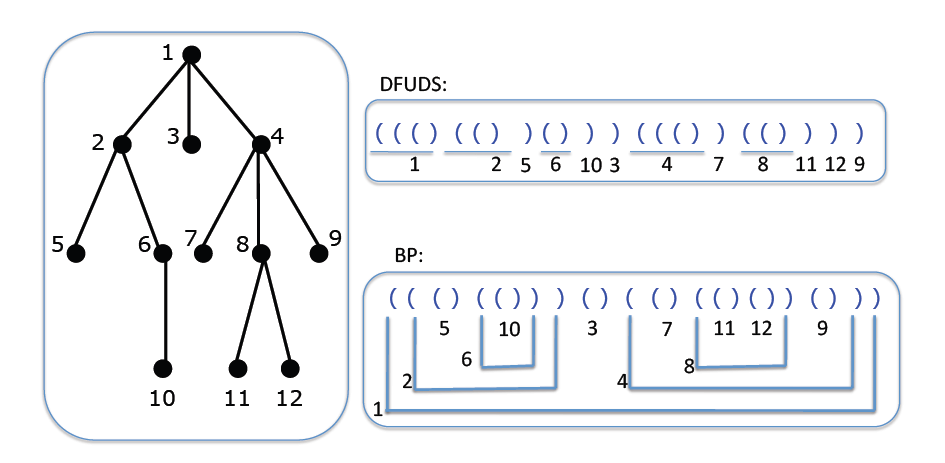
Figure 1: BP and DFUDS encodings of ordinal trees.

Succinct Ordinal Tree Representations.

Table 1 gives a subset of operations that are supported by various ordinal tree representations (see [19] for other operations).

Table 1: A list of operations on ordinal trees. In all cases below, if the value returned by the operation is not defined (e.g. performing $\text{parent}()$ on the root of the tree) an appropriate “null” value is returned.

Operation	Return Value
$\text{parent}(x)$	the parent of node $x$
$\text{child}(x,i)$	the $i$-th child of node $x$, for $i\geq 1$
$\text{next-sibling}(x)$	the next sibling of $x$
$\text{previous-sibling}(x)$	the previous sibling of $x$
$0pt(x)$	the depth of node $x$
$\text{select}_{o}(j)$	the $j$-th node in $o$-order, for $o\in\{\text{preorder},\text{postorder},$
	$\text{preorder-right},\text{postorder-right}\}$
$\text{leftmost-leaf}(x)$	the leftmost leaf of the subtree rooted at node $x$
$\text{rightmost-leaf}(x)$	the rightmost leaf of the subtree rooted at node $x$
$\text{subtree-size}(x)$	the size of the subtree rooted at node $x$ (excluding $x$ itself)
$\text{LCA}(x,y)$	the lowest common ancestor of the nodes $x$ and $y$
$\text{level-ancestor}(x,i)$	the ancestor of node $x$ at depth $d-i$, where $d=0pt(x)$, for $i\geq 0$

Theorem 1 ([22])

There is a succinct ordinal tree representation that supports all operations in Table 1 in $O(1)$ time and uses $2n+n/(\log n)^{O(1)}$ bits of space, where $n$ denotes the number of nodes in the represented ordinal tree.

2 Succinct Binary Trees Via Ordinal Trees

We describe succinct binary tree representations which are based on ordinal tree representations. In other words, we present a method that transforms a binary tree to an ordinal tree (indeed we study several and similar transformations) with properties used to simulate various operations on the original binary tree. We show that using known succinct ordinal tree representations from the literature, we can build succinct binary tree representations that have not yet been discovered. We also introduce a relationship between two standard ordinal tree encodings (BP and DFUDS) and study how this relationship can be utilized in our binary tree representations.

2.1 Transformations

We define four transformations $\tau_{1}$, $\tau_{2}$, $\tau_{3}$, and $\tau_{4}$ that transform a binary tree into an ordinal tree. We describe the $i$-th transformation by stating how we generate the output ordinal tree $T_{i}$ given an input binary tree $T_{b}$. Let $n$ be the number of nodes in $T_{b}$. The number of nodes in each of $T_{1}$, $T_{2}$, $T_{3}$, and $T_{4}$ is $n+1$, where each node corresponds to a node in $T_{b}$ except the root (think of the root as a dummy node). In the following, we show the correspondence between the nodes in $T_{b}$ and the nodes in $T_{i}$ by using the notation $\tau_{i}(\text{$u$})=\text{$v$}$, which means the node $u$ in $T_{b}$ corresponds to the node $v$ in $T_{i}$. Given a node $u$ in $T_{b}$, and its corresponding node $v$ in $T_{i}$, we show which nodes in $T_{i}$ correspond to the left and right children of $u$:

$\tau_{1}(\text{left-child$(u)$})=\text{first-child$(v)$}$	$\tau_{1}(\text{right-child$(u)$})=\text{next-sibling$(v)$}$
$\tau_{2}(\text{left-child$(u)$})=\text{last-child$(v)$}$	$\tau_{2}(\text{right-child$(u)$})=\text{previous-sibling$(v)$}$
$\tau_{3}(\text{left-child$(u)$})=\text{next-sibling$(v)$}$	$\tau_{3}(\text{right-child$(u)$})=\text{first-child$(v)$}$
$\tau_{4}(\text{left-child$(u)$})=\text{previous-sibling$(v)$}$	$\tau_{4}(\text{right-child$(u)$})=\text{last-child$(v)$}$

The example in Figure 2 shows a binary tree which is transformed to an ordinal tree by each of the four transformations. Notice that $T_{2}$ and $T_{4}$ are the mirror images of $T_{1}$ and $T_{3}$, respectively.

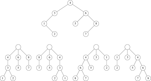
Figure 2: Top: a binary tree, nodes numbered in inorder. Bottom from left to right: the ordinal trees $T_{1}$, $T_{2}$, $T_{3}$, $T_{4}$. A node with number $k$ in the binary tree corresponds to the node with the same number $k$ in the ordinal trees. Notice that the roots of the ordinal trees do not correspond to any node in the binary tree.

2.2 Effect of Transformations on Orderings

It is clear that the order in which the nodes appear in $T_{b}$ is different from the node ordering in each of $T_{1}$, $T_{2}$, $T_{3}$, and $T_{4}$; however there is a surprising relation between these orderings. Consider the three standard orderings inorder, preorder, and postorder on binary trees and ordinal trees. While preorder and postorder arrange the nodes from left to right by default, we define their symmetries which arrange the nodes from right to left: preorder-right and postorder-right (i.e., visiting the children of each node from right to left in traversals). Each of the four transformations maps two of the binary tree orderings to two of the ordinal tree orderings. For example, if the first transformation maps inorder to postorder, that means a node with inorder rank $k$ in $T_{b}$ corresponds to a node with postorder rank $k$ in $T_{1}$. In the following, we show all of these mappings ($-1$ means that the mapping is off by 1, due to the presence of the dummy root):

$\tau_{1}$:	$\text{inorder}\ \rightarrow\text{postorder}$	$\text{preorder}\ \rightarrow\text{preorder}\ -1$
$\tau_{2}$:	$\text{inorder}\ \rightarrow\text{postorder-right}$	$\text{preorder}\ \rightarrow\text{preorder-right}\ -1$
$\tau_{3}$:	$\text{inorder}\ \rightarrow\text{preorder-right}-1$	$\text{postorder}\ \rightarrow\text{postorder-right}$
$\tau_{4}$:	$\text{inorder}\ \rightarrow\text{preorder}-1$	$\text{postorder}\rightarrow\text{postorder}$

2.3 Effect of Transformations on Ordinal Tree Encodings

The four transformation methods define four ordinal trees $T_{1}$, $T_{2}$, $T_{3}$, $T_{4}$ (from a given binary tree) which may look completely different, however they have relationships. In the following, we show a pairwise connection between $T_{1}$ and $T_{3}$ and between $T_{2}$ and $T_{4}$.

From paths to siblings and vice versa.

Recall the following transformation functions on the binary tree nodes:

$\tau_{1}(\text{left-child$(u)$})=\text{first-child$(v)$}$	$\tau_{1}(\text{right-child$(u)$})=\text{next-sibling$(v)$}$
$\tau_{3}(\text{left-child$(u)$})=\text{next-sibling$(v)$}$	$\tau_{3}(\text{right-child$(u)$})=\text{first-child$(v)$}$

If we combine the above functions, we can conclude the following:

$$\text{first-child$(v)$ in $\tau_{1}$}=\text{next-sibling$(v)$ in $\tau_{3}$}$$

$$\text{next-sibling$(v)$ in $\tau_{1}$}=\text{first-child$(v)$ in $\tau_{3}$}$$

The above relation yields a connection between paths in $T_{1}$ and the siblings in $T_{3}$. Consider any downward path $(u_{1},u_{2},\ldots,u_{k})$ in $T_{1}$, where $u_{1}$ is the $i$-th child of a node for any $i>1$ and all $u_{2},\ldots,u_{k}$ are the first child of their parents. All the nodes $u_{1},u_{2},\ldots,u_{k}$ become siblings in $T_{3}$ and they are all the children of a node which corresponds to the previous-sibling of $u_{1}$ in $T_{1}$. Also, if $u_{1}$ is the root of $T_{1}$ then $u_{1}$ corresponds to the root in $T_{3}$ and all $u_{2},\ldots,u_{k}$ become the children of the root of $T_{3}$. The paths in $T_{3}$ are related to siblings in $T_{1}$ in a similar way. Also, a similar connection exists between $T_{2}$ and $T_{4}$ with the only difference that first child, next sibling, and previous sibling should be turned into last child, next sibling, and previous sibling in order.

From BP to DFUDS and vice versa.

Section 1.1 introduced two standard ordinal tree encodings: BP and DFUDS. The relation between paths and siblings in the different types of transforms suggests a relation between the BP and DFUDS sequences of these transformations, as paths of the kind considered above lead to consecutive sequences of parentheses, which in DFUDS can be viewed as the encoding of a group of siblings. We now formalize this intuition. Let DFUDS-RtL be the DFUDS sequence where the children of every node are visited from right to left.

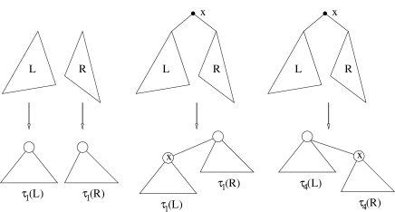
Figure 3: Illustrating how the result of transformations $\tau_{1}$ and $\tau_{4}$ on a binary tree with root $x$, left subtree $L$ and right subtree $R$ can be obtained from the transformations $\tau_{1}$ and $\tau_{4}$ on $L$ and $R$.

Theorem 2

For any binary tree $T_{b}$, let $T_{i}$ denote the result of $\tau_{i}$ applied to $T_{b}$. Then:

1. The BP sequences of $T_{1}$ and $T_{3}$ are the reverses of the BP sequences of $T_{2}$ and $T_{4}$, respectively.

2. The DFUDS sequences of $T_{1}$ and $T_{3}$ are equal to the DFUDS-RtL sequences of $T_{2}$ and $T_{4}$, respectively.

3. The BP sequence of $T_{1}$ is equal to the DFUDS sequence of $T_{4}$.

4. The BP sequence of $T_{2}$ is equal to the DFUDS sequence of $T_{3}$.

• (1) and (2) follow directly from the definitions of the transformations.

  We prove (3) by induction ((4) is analogous). For any ordinal tree $T$ denote by BP($T$) and DFUDS($T$) the BP and DFUDS encodings of $T$. For the base case, if $T_{b}$ consists of a singleton node, then BP($T_{1}$) = DFUDS($T_{4}$) = (()). Before going to the inductive case, observe that for any binary tree $T$, BP($\tau_{i}$($T$)) is a string of the form $(Y)$, where the parenthesis pair enclosing $Y$ represents the dummy root of $\tau_{i}$($T$), and $Y$ is the BP representation of the ordered forest obtained by deleting the dummy root. On the other hand, DFUDS($\tau_{i}$(T)), which can also be viewed as a string of the form $(Y)$, is interpreted differently: the first open parenthesis is a dummy, while $Y)$ is the core DFUDS representation of the entire tree $\tau_{i}$($T$), including the dummy root.

  Now let $T_{b}$ be a binary tree with root $x$, left subtree $L$ and right subtree $R$. By induction, BP($\tau_{1}$($L$)) = DFUDS($T_{4}$($L$)) = $(Y)$ and BP($T_{1}$($R$)) = DFUDS($T_{4}$($R$)) = $(Z)$. Note that $T_{1}$ is obtained as follows. Replace the dummy root of $\tau_{1}$($L$) by $x$, and insert $x$ as the first child of the dummy root of $\tau_{1}$($R$) (see Figure 3). Thus, BP($T_{1}$) = $((Y)Z)$.

  Next, $T_{4}$ is obtained as follows: replace the dummy root of $\tau_{4}$($R$) by $x$, and insert $x$ as the last child of the dummy root of $\tau_{4}$($L$) (see Figure 3). The core DFUDS representation of $T_{4}$ (i.e. excluding the dummy open parenthesis) is obtained as follows: add an open parenthesis to the front of the core DFUDS representation of $\tau_{4}$($L$), to indicate that the root of $\tau_{4}$($L$), which is also the root of $T_{4}$, has one additional child. This gives the parenthesis sequence $(Y)$. To this we append the core DFUDS representation of $\tau_{4}$($R$), giving $(Y)Z)$. Now we add the dummy open parenthesis, giving $((Y)Z)$, which is the same as BP($T_{1}$). $\blacksquare$

2.4 Succinct Binary Tree Representations

We consider the problem of encoding a binary tree in a succinct data structure that supports the operations: left-child, right-child, parent, subtree-size, LCA, inorder, and one of preorder or postorder (we give two data structures supporting preorder and two other ones supporting postorder). We design such a data structure by transforming the input binary tree into an ordinal tree using any of the transformations $\tau_{1}$, $\tau_{2}$, $\tau_{3}$, or $\tau_{4}$, and then encoding the ordinal tree by a succinct data structure that supports appropriate operations. For each of the four ordinal trees that can be obtained by the transformations, we give a set of algorithms, each performs one of the binary tree operations. In other words, we show how each of the binary tree operations can be performed by ordinal tree operations. Here, we show this for transformation $\tau_{1}$, and later in the section we present the pseudocode for all the transformations. In the following, $u$ denotes any given node in a binary tree $T_{b}$, and $\tau_{1}(u)$ denotes the node corresponding to $u$ in $T_{1}$:

left-child.

The left child of $u$ is the first child of $\tau_{1}(u)$, which can be determined by the operation child($1,\tau_{1}(u)$) on $T_{1}$.

right-child.

The right child of $u$ is the next sibling of $\tau_{1}(u)$, which can be determined by the operation $\text{next-sibling}(\tau_{1}(u))$ on $T_{1}$.

parent.

To determine the parent of $u$, there are two cases: (1) if $\tau_{1}(u)$ is the first child of its parent, then the answer is the parent of $\tau_{1}(u)$ to be determined by parent($\tau_{1}(u)$) on $T_{1}$; (2) if $\tau_{1}(u)$ is not the first child of its parent, then the answer is the previous sibling of $\tau_{1}(u)$ to be determined by the operation $\text{previous-sibling}(\tau_{1}(u))$ on $T_{1}$.

subtree-size.

The subtree size of $u$ is equal to the subtree size of $\tau_{1}(u)$ plus the sum of the subtree sizes of all the siblings to the right of $\tau_{1}(u)$. Let $\ell$ be the rightmost leaf in the subtree of the parent of $\tau_{1}(u)$. To obtain the above sum, we subtract the preorder number of $\tau_{1}(u)$ from the preorder number of $\ell$, which can be performed using the operations $\text{rightmost-leaf}(\text{parent}(\tau_{1}(u)))$ and preorder.

LCA

Let $w$ be the LCA of the two nodes $u$ and $v$ in $T_{b}$. We want to find $w$ given $u$ and $v$, assuming w.l.o.g. that $\text{\text{preorder}}(u)$ is smaller than $\text{\text{preorder}}(v)$. Let lca be the LCA of $\tau_{1}(u)$ and $\tau_{1}(v)$ in $T_{1}$. Observe that lca is a child of $\tau_{1}(w)$ and an ancestor of $\tau_{1}(u)$. Thus, we only need to find the ancestor of $\tau_{1}(u)$ at level $i$, where $i-1$ is the depth of lca. To compute this, we utilize the operations LCA, 0pt, and level-ancestor on $T_{1}$.

See Tables 2 through 5 for the pseudocode of all the binary tree operations on all four transformations.

Table 2: Binary tree operations performed using ordinal tree operations for transformation $\tau_{1}$. The ordinal tree operations preorder, preorder-right postorder, and postorder-right are the same as $\text{select}_{o}$ for different values of $o$ (refer to Table 1).

$\text{\text{inorder}}(u)$: return $\text{\text{postorder}}(\tau_{1}(u))$	$\text{\text{preorder}}(u)$: return $\text{\text{preorder}}(\tau_{1}(u))$ - 1
left-child($u$): return child($1,\tau_{1}(u)$)	right-child($u$): return $\text{next-sibling}(\tau_{1}(u))$
parent($u$): $v$ = $\text{previous-sibling}(\tau_{1}(u))$ if $v$ $\neq$ NULL return $v$ else return parent($\tau_{1}(u)$) subtree-size($u$): $\ell$ = $\text{rightmost-leaf}(\text{parent}(\tau_{1}(u)))$ return $\text{\text{preorder}}(\ell)$ - $\text{\text{preorder}}(\tau_{1}(u))$	//assume $\text{\text{preorder}}(u)$ < $\text{\text{preorder}}(v)$ LCA($u,v$): lca = LCA($\tau_{1}(u),\tau_{1}(v)$) if lca == $\tau_{1}(u)$ return lca if lca == parent($\tau_{1}(u)$) return $\tau_{1}(u)$ $i$ = $\text{depth}(\text{lca})$+1 return level-ancestor($\tau_{1}(u),i$)

Table 3: Binary tree operations performed using ordinal tree operations for transformation $\tau_{2}$. The ordinal tree operations preorder, preorder-right postorder, and postorder-right are the same as $\text{select}_{o}$ for different values of $o$ (refer to Table 1).

$\text{\text{inorder}}(u)$: return $\text{\text{postorder-right}}(\tau_{2}(u))$	$\text{\text{preorder}}(u)$: return $\text{\text{preorder-right}}(\tau_{2}(u))$ - 1
left-child($u$): $d$ = $\text{degree}(\tau_{2}(u))$ return child($d,\tau_{2}(u)$)	right-child($u$): return $\text{previous-sibling}(\tau_{2}(u))$
parent($u$): $v$ = $\text{next-sibling}(\tau_{2}(u))$ if $v$ $\neq$ NULL return $v$ else return parent($\tau_{2}(u)$) subtree-size($u$): $\ell$ = $\text{leftmost-leaf}(\text{parent}(\tau_{2}(u)))$ return $\text{\text{preorder-right}}(\ell)$ - $\text{\text{preorder-right}}(\tau_{2}(u))$	//assume $\text{\text{preorder}}(u)$ > $\text{\text{preorder}}(v)$ LCA($u,v$): lca = LCA($\tau_{2}(u),\tau_{2}(v)$) if lca == $\tau_{2}(u)$ return lca if lca == parent($\tau_{2}(u)$) return $\tau_{2}(u)$ $i$ = $\text{depth}(\text{lca})$+1 return level-ancestor($\tau_{2}(u),i$)

Table 4: Binary tree operations performed using ordinal tree operations for transformation $\tau_{3}$. The ordinal tree operations preorder, preorder-right postorder, and postorder-right are the same as $\text{select}_{o}$ for different values of $o$ (refer to Table 1).

$\text{\text{inorder}}(u)$: return $\text{\text{preorder-right}}(\tau_{3}(u))$ - 1	$\text{\text{postorder}}(u)$: return $\text{\text{postorder}}(\tau_{3}(u))$
left-child($u$): return $\text{next-sibling}(\tau_{3}(u))$	right-child($u$): return child($1,\tau_{3}(u)$)
parent($u$): $v$ = $\text{previous-sibling}(\tau_{3}(u))$ if $v$ $\neq$ NULL return $v$ else return parent($\tau_{3}(u)$) subtree-size($u$): $\ell$ = $\text{rightmost-leaf}(\text{parent}(\tau_{3}(u)))$ return $\text{\text{postorder-right}}(u)$ - $\text{\text{postorder-right}}(\tau_{3}(\ell))$	//assume $\text{\text{preorder}}(u)$ < $\text{\text{preorder}}(v)$ LCA($u,v$): lca = LCA($\tau_{3}(u),\tau_{3}(v)$) if lca == $\tau_{3}(u)$ return lca if lca == parent($\tau_{3}(u)$) return $\tau_{3}(u)$ $i$ = $\text{depth}(\text{lca})$+1 return level-ancestor($\tau_{3}(u),i$)

Table 5: Binary tree operations performed using ordinal tree operations for transformation $\tau_{4}$. The ordinal tree operations preorder, preorder-right postorder, and postorder-right are the same as $\text{select}_{o}$ for different values of $o$ (refer to Table 1).

$\text{\text{inorder}}(u)$: return $\text{\text{preorder}}(\tau_{4}(u))$ - 1	$\text{\text{postorder}}(u)$: return $\text{\text{postorder}}(\tau_{4}(u))$
left-child($u$): return $\text{previous-sibling}(\tau_{4}(u))$	right-child($u$): $d$ = $\text{degree}(\tau_{4}(u))$ return child($d,\tau_{4}(u)$)
parent($u$): $v$ = $\text{next-sibling}(\tau_{4}(u))$ if $v$ $\neq$ NULL return $v$ else return parent($\tau_{4}(u)$) subtree-size($u$): $\ell$ = $\text{leftmost-leaf}(\text{parent}(\tau_{4}(u)))$ return $\text{\text{postorder}}(u)$ - $\text{\text{postorder}}(\tau_{4}(\ell))$	//assume $\text{\text{preorder}}(u)$ > $\text{\text{preorder}}(v)$ LCA($u,v$): lca = LCA($\tau_{4}(u),\tau_{4}(v)$) if lca == $\tau_{4}(u)$ return lca if lca == parent($\tau_{4}(u)$) return $\tau_{4}(u)$ $i$ = $\text{depth}(\text{lca})$+1 return level-ancestor($\tau_{4}(u),i$)

Theorem 3

There is a succinct binary tree representation of size $2n+n/(\log n)^{O(1)}$ bits that supports all the operations left-child, right-child, parent, subtree-size, LCA, inorder, and one of preorder or postorder in $O(1)$ time, where $n$ denotes the number of nodes in the represented binary tree.

• We can use any of the transformations $\tau_{1}$, $\tau_{2}$, $\tau_{3}$, or $\tau_{4}$ and use any ordinal tree representation that uses $2n+n/(\log n)^{O(1)}$ bits and supports the operations required by our algorithms (Theorem 1). $\blacksquare$

2.5 BP for Binary Trees (Zaks’ sequence)

Let $T_{b}$ be a binary tree which is transformed to the ordinal tree $T_{1}$ by the first transformation $\tau_{1}$. We show that the BP sequence of $T_{1}$ is a special sequence for $T_{b}$. This sequence is called Zaks’ sequence, and our transformation methods show that Zaks’ sequence can be indeed used to encode binary trees into a succinct data structure that supports various operations. In the following, we give a definition for Zaks’ sequence of $T_{b}$ and we show that it is indeed equal to the BP sequence of $T_{1}$.

Zaks’ sequence.

Initially, extend the binary tree $T_{b}$ by adding external nodes wherever there is a missing child. Now, label the internal nodes with an open parenthesis, and the external nodes with a closing parenthesis. Zaks’ sequence of $T_{b}$ is derived by traversing $T_{b}$ in preorder and printing the labels of the visited nodes. If $T_{b}$ has $n$ nodes, Zaks’ sequence is of length $2n+1$. If we insert an open parenthesis at the beginning of Zaks’ sequence, then it becomes a balanced-parentheses sequence. Notice that Zaks’ sequence is different from Jacobson’s [15] approach where $T_{b}$ is traversed in level-order. See Figure 4 for an example.

Each pair of matching open and close parentheses in Zaks’ sequence, except the extra open parenthesis at the beginning and its matching close parenthesis, is (conceptually) associated with a node in $T_{b}$. Observe that the open parentheses in the sequence from left to right correspond to the nodes in preorder, and the closing parentheses from left to right correspond to the nodes in inorder.

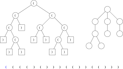
Figure 4: Illustrating the connection between Zaks’ sequence of $T_{b}$ and the BP sequence of $T_{1}$ (Left: A binary tree $T_{b}$; Right: The ordinal tree $T_{1}$ derived from applying transformation $\tau_{1}$ to $T_{b}$).

Zaks’ sequence and transformation $\tau_{1}$.

Zaks’ sequence of $T_{b}$ including the extra open parenthesis at the beginning is the same as the BP sequence of $T_{1}$. This is stated in the following lemma:

Theorem 4

An open parenthesis appended by Zaks’ sequence of a binary tree is the same as the BP sequence of the ordinal tree obtained by applying the first transformation $\tau_{1}$ to the binary tree.

• Let $T_{b}$ and $T_{1}$ be the binary tree and ordinal tree respectively, and let $S$ be the sequence of an open parenthesis appended by Zaks’ sequence of $T_{b}$. We prove the lemma by induction on the number of nodes in $T_{b}$.

  For the base case, If $T_{b}$ has only one node, then Zaks’ sequence of $T_{b}$ will be $())$ and the BP of $T_{1}$ will be $(())$. Take as the induction hypothesis that the lemma is correct for $T_{b}$ with less than $n$ nodes.

  In the inductive step, let $T_{b}$ have $n$ nodes. Let $u_{1},u_{2},\ldots,u_{k}$ be the right most path in $T_{b}$, where $1\leq k\leq n$. Let $l_{i}$ be the left subtree of $u_{i}$ for $1\leq i\leq k$. Thus, $S=((z_{1}(z_{2}\cdots(z_{k})$, where $z_{i}$ is Zaks’ sequence of $l_{i}$. Notice that the size of each $l_{i}$ is smaller than $n$. Therefore by the hypothesis, $(z_{i}$ is the BP sequence $b_{i}$ of the ordinal tree $\tau_{1}(l_{i})$. The ordinal tree $T_{1}$ has a dummy root which has $k$ subtrees which are identical to $\tau_{1}(l_{i})$ for $1\leq i\leq k$. Therefore, the BP sequence of $T_{1}$ is $(b_{1}b_{2}\cdots b_{k})$, where $b_{i}$ is the BP sequence of the subtree rooted at $\tau_{1}(u_{i})$. Thus, the BP sequence of $T_{1}$ is the same as $S$. $\blacksquare$

3 Cartesian Tree Construction in $o(n)$ Working Space

Given an array $A$, we now show how to construct one of the succinct tree representations implied in Theorem 3 in small working space. The model is that the array $A$ is present in read-only memory. There is a working memory, which is read-write, and the succinct Cartesian tree representation is written to a readable, but write-once, output memory. All memory is assumed to be randomly accessible.

A straightforward way to construct a succinct representation of a Cartesian tree is to construct the standard pointer-based representation of the Cartesian tree from the given array in linear time [9], and then construct the succinct representation using the pointer-based representation. The drawback of this approach is that the space used during the construction is $O(n\log n)$ bits, although the final structure uses only $O(n)$ bits. Fischer and Heun [8] show that the construction space can be reduced to $n+o(n)$ bits. In this section, we show how to improve the construction space to $o(n)$ bits. In fact, we first show that a parenthesis sequence corresponding to the Cartesian tree can be output in linear time using only $O(\sqrt{n}\log n)$ bits of working space; subsequently, using methods from [10] the auxiliary data structures can also be constructed in $o(n)$ working space.

Theorem 5

Given an array $A$ of $n$ values, let $T_{c}$ be the Cartesian tree of $A$. We can output BP($\tau_{4}$($T_{c}$)) in $O(n)$ time using $O(\sqrt{n}\log n)$ bits of working space.

• The algorithm reads $A$ from left to right and outputs a parenthesis sequence as follows: when processing $A[i]$, for $i=1,\ldots,n$ we compare $A[i]$ with all the suffix minima of $A[1..i-1]$—if $A[i]$ is smaller than $j\geq 0$ suffix minima, then we output the string $(\,)^{j}$. Finally we add the string $(\,)^{j+1}$ to the end, where $j$ is the number of suffix minima of $A[1..n]$.

  Given any ordinal tree $T$, define the post-order degree sequence parenthesis string obtained from $T$, denoted by PODS($T$), as follows. Traverse $T$ in post-order, and at each node that has $d$ children, output the bit-string $(\,)^{d}$. At the end, output an additional $)$. Let $T_{c}$ be the Cartesian tree of $A$ and for $i=1,\ldots,4$, let $T_{i}$ = $\tau_{i}$($T_{c}$) as before. Observe that in $T_{1}$, for $i=1,\ldots,n$, the children of the $i$-th node in post-order, which is the $i$-th node in $T_{c}$ in in-order and hence corresponds to $A[i]$, are precisely those suffix minima that $A[i]$ was smaller than when $A[i]$ was processed. Furthermore, the children of the (dummy) root of $T_{1}$ are the suffix maxima of $A[1..n]$. Thus, the string output by the above pre-processing of $A$ is PODS($T_{1}$).

  We now show that PODS($T_{1}$) = BP($T_{4}$). The proof is along the lines of Theorem 2. If $L$ and $R$ denote the left subtree of the root of $T_{c}$, assume inductively that BP($\tau_{4}$($L$)) = PODS($\tau_{1}$($L$)) = $(Y)$ and BP($\tau_{4}$($R$)) = PODS($\tau_{1}$($L$)) = $(Z)$. Using the reasoning in Theorem 2 (summarized in Figure 3) we see immediately that BP($T_{4}$) = $(Y(Z))$, and by a reasoning similar to the one used for DFUDS in Theorem 2, it is easy to see that PODS($T_{1}$) = $(Y(Z))$ as well, as required.

  While the straightforward approach would be to maintain a linked list of the locations of the current suffix minima, this list could contain $\Theta(n)$ locations and could take $\Theta(n\log n)$ bits. Our approach is to use the output string itself to encode the positions of the suffix minima. One can observe that if the output string is created by the above process, it will be of the form $(b_{1}(...(b_{k}$ where each $b_{i}$ is a (possibly empty) maximal balanced parenthesis string – the remaining parentheses are called unmatched. It is not hard to see that the unmatched parentheses encode the positions of the suffix minima in the sense that if the unmatched parentheses (except the opening one) are the $i_{1},i_{2}\ldots,i_{k}$-th opening parentheses in the current output sequence then the positions $i_{1}-1,\ldots,i_{k}-1$ are precisely the suffix minima positions. Our task is therefore to sequentially access the next unmatched parenthesis, starting from the end, when adding the new element $A[i+1]$. We conceptually break the string into blocks of size $\lfloor\sqrt{n}\rfloor$. For each block that contains at least one unmatched parenthesis, store the following information:

  • its block number (in the original parenthesis string) and the total number of open parenthesis in the current output string before the start of the block.

  • the position $p$ of the rightmost parenthesis in the block, and the number of open parentheses before it in the block.

  • a pointer to the next block with at least one unmatched parenthesis.

  This takes $O(\log n)$ bits per block, which is $O(\sqrt{n}\log n)$ bits.

  • For the rightmost block (in which we add the new parentheses), keep positions of all the unmatched parentheses: the space for this is also $O(\sqrt{n}\log n)$ bits.

  When we process the next element of $A$, we compare it with unmatched parentheses in the rightmost block, which takes $O(1)$ time per unmatched parenthesis that we compared the new element with, as in the algorithm of [9]. Updating the last block is also trivial. Suppose we have compared $A[i]$ and found it smaller than all suffix maxima in the rightmost block. Then, using the linked list, we find the rightmost unmatched parenthesis (say at position $p$) in the next block in the list, which takes $O(1)$ time, and compare with it (this is also $O(1)$ time). If $A[i]$ is smaller, then sequentially scan this block leftwards starting at position $p$, skipping over a maximal BP sequence to find the next unmatched parenthesis in that block. The time for this sequential scan is $O(n)$ overall, since we never sequentially scan the same parenthesis twice. Updating the blocks is straightforward. Thus, the creation of the output string can be done in linear time using $O(\sqrt{n}\log n)$ bits of working memory. $\blacksquare$

References

- [1] M. I. Abouelhoda, S. Kurtz, and E. Ohlebusch. Replacing suffix trees with enhanced suffix arrays. Journal of Discrete Algorithms, 2(1):53–86, 2004.
- [2] D. Arroyuelo, R. Cánovas, G. Navarro, and K. Sadakane. Succinct trees in practice. In G. E. Blelloch and D. Halperin, editors, ALENEX, pages 84–97. SIAM, 2010.
- [3] D. Benoit, E. D. Demaine, J. I. Munro, R. Raman, V. Raman, and S. S. Rao. Representing trees of higher degree. Algorithmica, 43(4):275–292, 2005.
- [4] G. Chen, S. J. Puglisi, and W. F. Smyth. Lempel-Ziv factorization using less time and space. Mathematics in Computer Science, 1:605–623, 2008.
- [5] P. Davoodi, G. Navarro, R. Raman, and S. R. Satti. Encoding range minima and range top-2 queries. Philosphical Transactions of the Royal Society A, 372:20130131, 2014.
- [6] A. Farzan and J. I. Munro. A uniform approach towards succinct representation of trees. In Proc. 11th Scandinavian Workshop on Algorithm Theory, pages 173–184. Springer-Verlag, 2008.
- [7] A. Farzan, R. Raman, and S. S. Rao. Universal succinct representations of trees? In Proc. 36th International Colloquium on Automata, Languages and Programming, pages 451–462. Springer, 2009.
- [8] J. Fischer and V. Heun. Space-efficient preprocessing schemes for range minimum queries on static arrays. SIAM Journal on Computing, 40(2):465–492, 2011.
- [9] H. N. Gabow, J. L. Bentley, and R. E. Tarjan. Scaling and related techniques for geometry problems. In Proc. 16th annual ACM symposium on Theory of computing, pages 135–143. ACM Press, 1984.
- [10] R. F. Geary, N. Rahman, R. Raman, and V. Raman. A simple optimal representation for balanced parentheses. Theoretical Computer Science, 368(3):231–246, 2006.
- [11] L. Georgiadis and R. E. Tarjan. Finding dominators revisited: extended abstract. In Proc. 15th Annual ACM-SIAM symposium on Discrete algorithms, pages 869–878. SIAM, 2004.
- [12] S. Gog, T. Beller, A. Moffat, and M. Petri. From theory to practice: Plug and play with succinct data structures. CoRR, abs/1311.1249, 2013.
- [13] R. Grossi and G. Ottaviano. Design of practical succinct data structures for large data collections. In V. Bonifaci, C. Demetrescu, and A. Marchetti-Spaccamela, editors, SEA, volume 7933 of Lecture Notes in Computer Science, pages 5–17. Springer, 2013.
- [14] C. S. Iliopoulos, M. Crochemore, M. Kubica, M. S. Rahman, and T. Walen. Improved algorithms for the range next value problem and applications. In Proc. 25th International Symposium on Theoretical Aspects of Computer Science, volume 1 of Leibniz International Proceedings in Informatics, pages 205–216. Schloss Dagstuhl - Leibniz-Zentrum fuer Informatik, 2008.
- [15] G. Jacobson. Succinct Static Data Structures. PhD thesis, Carnegie Mellon University, Pittsburgh, PA, USA, 1989.
- [16] J. I. Munro and V. Raman. Succinct representation of balanced parentheses and static trees. SIAM Journal on Computing, 31(3):762–776, 2001.
- [17] S. Muthukrishnan. Efficient algorithms for document retrieval problems. In Proc. 13th Annual ACM-SIAM symposium on Discrete algorithms, pages 657–666. SIAM, 2002.
- [18] M. Patrascu. Succincter. In FOCS, pages 305–313. IEEE Computer Society, 2008.
- [19] R. Raman and S. S. Rao. Succinct representations of ordinal trees. In A. Brodnik, A. López-Ortiz, V. Raman, and A. Viola, editors, Space-Efficient Data Structures, Streams, and Algorithms, volume 8066 of Lecture Notes in Computer Science, pages 319–332. Springer, 2013.
- [20] K. Sadakane. Compressed suffix trees with full functionality. Theory of Computing Systems, 41(4):589–607, 2007.
- [21] K. Sadakane. Succinct data structures for flexible text retrieval systems. Journal of Discrete Algorithms, 5(1):12–22, 2007.
- [22] K. Sadakane and G. Navarro. Fully-functional succinct trees. In Proc. 21st Annual ACM-SIAM Symposium on Discrete Algorithms, pages 134–149. SIAM, 2010.
- [23] S. Saxena. Dominance made simple. Information Processing Letters, 109(9):419–421, 2009.
- [24] N. Välimäki and V. Mäkinen. Space-efficient algorithms for document retrieval. In Proc. 18th Annual Symposium on Combinatorial Pattern Matching, volume 4580 of LNCS, pages 205–215. Springer-Verlag, 2007.
- [25] J. Vuillemin. A unifying look at data structures. Communications of the ACM, 23(4):229–239, 1980.
- [26] S. Zaks. Lexicographic generation of ordered trees. Theor. Comput. Sci., 10:63–82, 1980.