Human Motion Capture Data
Tailored Transform Coding

Abstract

Human motion capture (mocap) is a widely used technique for digitalizing human movements. With growing usage, compressing mocap data has received increasing attention, since compact data size enables efficient storage and transmission. Our analysis shows that mocap data have some unique characteristics that distinguish themselves from images and videos. Therefore, directly borrowing image or video compression techniques, such as discrete cosine transform, does not work well. In this paper, we propose a novel mocap-tailored transform coding algorithm that takes advantage of these features. Our algorithm segments the input mocap sequences into clips, which are represented in 2D matrices. Then it computes a set of data-dependent orthogonal bases to transform the matrices to frequency domain, in which the transform coefficients have significantly less dependency. Finally, the compression is obtained by entropy coding of the quantized coefficients and the bases. Our method has low computational cost and can be easily extended to compress mocap databases. It also requires neither training nor complicated parameter setting. Experimental results demonstrate that the proposed scheme significantly outperforms state-of-the-art algorithms in terms of compression performance and speed.

I Introduction

Human motion capture (mocap) is the process to digitally record human movement using information (e.g., angle and 3D coordinate) of a set of key points (i.e., markers or joints). As a highly successful technique, it has been extensively used in entertainment, medical, sports and military applications [14]. The output of a mocap session is the trajectories of a set of key points. An accurate motion capture requires tracking a large number of markers at very high frequency, therefore, the generated mocap data is usually bulky, which poses a challenge to both storage and transmission. It is highly desirable to develop an efficient method for compressing mocap data.

The primary goal of data compression is to reduce the redundancy or correlation in the data. As an effective tool for data decorrelation, transform coding maps the original data into the transform domain, in which the transform coefficients have significantly less dependency than the original data. Since most of the energy concentrates on a small portion of the transform domain, compression can be achieved by discarding the less-important information (i.e., setting the smallest coefficients to be zeros). To recover the data, one simply applies the inverse transformation to the transform coefficients. Representative transform coding methods are the Karhunen-Loeve Transform (KLT), Principal Component Analysis (PCA) (or more generally, Singular Value Decomposition (SVD)), Discrete Wavelet Transform (DWT), and Discrete Cosine Transform (DCT). Among them, the 2D DCT and DWT methods are extremely successful in images/videos compression, e.g., JPEG-2000 and H.264/AVC, due to the locally smooth nature in images and/or videos, leading to most transform coefficients occupying low frequencies. Since human mocap data can be naturally represented by a 2D matrix, where each row corresponds to the trajectory of a marker, one may simply borrow the existing image-based transform coding methods to mocap data. Unfortunately, our analysis shows that mocap data have some unique characteristics that distinguish themselves from images and videos. Therefore, directly applying DCT or DWT does not work well.

This paper presents a novel transform coding method for compressing human mocap data. Observing that a subset of a long mocap sequence exhibits stronger data dependency, we segment the input data into a set of clips, and represent each clip by a matrix, where each row is the trajectory of a marker. Note that mocap data is smooth in the dimension of time, since each marker’s trajectory is a smooth curve in $\mathbb{R}^{3}$. See Fig. 1. However, the columns exhibit much less smoothness due to the complex nature of human motion. Based on these observations, our transform coding method adopts a data-dependent left transformation and a data-independent right transformation, where the former is to reduce redundancy among the non-smooth columns and the latter is to decorrelate the smooth rows. Our transform coding is very effective, since it produces only a small number of coefficients in the transform domain. Moreover, our method has low computational cost and can be easily extended for mocap database compression. Unlike the existing approaches to mocap data compression, our method requires neither training nor complicated parameter setting. Experimental results demonstrate that the proposed method significantly outperforms state-of-the-art algorithms in terms of speed and compression performance.

The rest of this paper is organized as follows: Section II briefly reviews previous work on mocap data compression. Section III analyzes the human mocap data and shows its unique features, which distinguish themselves from natural images and videos. Then Section IV presents our tailored transform coding, which is further generalized to mocap database in Section V. Section VI evaluates our method and presents the experimental results. Finally, Section VII concludes this paper and points out some promising future direction as well as the potential of our scheme on other applications.

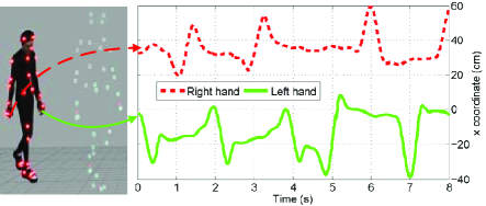
Figure 1: Marker-based motion capture device records the movement of a person by tracking the markers wore on his or her joints. Each marker trajectory is a smooth curve in $\mathbb{R}^{3}$. For better visualization, we only plot the $x$ coordinate. The left photo is taken from %****␣human_mocap_compression_arxiv.tex␣Line␣175␣****http://nward.com/ict/blender/mocap.htm

II Previous Work

Compared to the widely-studied video/image compression, mocap data compression is a relatively young field. Liu et al. [1] partitioned a mocap data sequence into subsequences, and then applied the PCA to keyframes of each subsequence separately. Fitting fixed-length short mocap clips using Bézier curves, Arikan [6] performed clustered PCA to reduce their dimensionality. Observing that human motion often exhibits repeated patterns, Lin et al. [11] applied the PCA to the repeated motion and interpolated the marker trajectories. Tournier et al. [10] proposed a principal geodesic analysis (PGA)-based approach, which stores only some poses manifolds, the end-effectors as well as root joint’s trajectories and orientations. The motion can be recovered through Inverse Kinematics (IK) in a lossy manner.

Beaudoin et al. [3] applied 1D DWT to joint angles, and the WT coefficients were optimally selected by taking the visual artifacts into account. This method was futher improved by Firouzmanesh et al. [21]. Preda and Preteux [15] adopted temporal prediction and spatial 1D DCT in MPEG-4 bone-based animation (BBA) to remove redundancy. Using fuzzy clustering, Chew et al. [9] reorganized mocap data into matrices with strong local correlation, and then adopted the JPEG-2000 (employing 2D DWT) to encode them.

Chattopadhyay et al. [2] proposed a novel model-based indexing method, which exploits structural information derived from the skeletal virtual human model. Gu et al. [12] compressed human mocap data by hierarchical structure construction and motion pattern indexing. They also built a mocap database for each meaningful body part and a sequence of mocap data can be efficiently represented as a series of motion pattern indices. Taking advantage of the sparsity of mocap data in the action domain and time domain, Li et al. [8] proposed a learning-based scheme to train a set of shift-invariant basis functions, on which the mocap sequences can be projected, leading to sparse coefficients. Lim and Thalmann [4], Xiao et al. [5] and Kim et al. [7] proposed keyframe-based methods, which extract a few representative frames, and then represent the whole mocap sequence by interpolating these keyframes. Zhu et al. [13] represented human motion data in the quaternion space so that human rotational motion data can be decomposed into the dictionary part and the sparse weight part. Le et al. [16] computed optimized marker layouts for capturing facial expression as optimization of characteristic control points from a set of high-resolution, ground truth facial mesh sequences. Hou et al. [22] proposed a tensor representation, in which mocap clips were assembled into a third-order tensor. They applied the canonical polyadic decomposition to explore correlation

Instead of using the standard application-independent transformations, our transform coding method is tailored to mocap data by taking advantage of their unique properties (see Section 3). As a result, our method outperforms the existing techniques in terms of both speed and compression performance. Moreover, our method has good scalability so that it works for both a single motion sequence and a set of mocap sequences, i.e., mocap database.

III Human Mocap Data Analysis

As pointed in [1, 6, 11], compressing the position-based mocap data has advantages over the hierarchical angle-based representation, which exhibits intrinsic nonlinearity. Besides, the hierarchical structure results in the accumulation of errors along the chain of joint angles, resulting in significant jerkiness [9]. Therefore, we use the position-based human mocap data in this paper. We represent a human mocap sequence by a matrix $\mathbf{M}\in\mathbb{R}^{3n\times f}$, i.e.,

$$\centering\mathbf{M}=\left(\begin{array}[]{cccc}x_{1,1}&x_{1,2}&\cdots&x_{1,f}\\ \vdots&\vdots&\ddots&\vdots\\ x_{n,1}&x_{n,2}&\cdots&x_{n,f}\\ y_{1,1}&y_{1,2}&\cdots&y_{1,f}\\ \vdots&\vdots&\ddots&\vdots\\ y_{n,1}&y_{n,2}&\cdots&y_{n,f}\\ z_{1,1}&z_{1,2}&\cdots&z_{1,f}\\ \vdots&\vdots&\ddots&\vdots\\ z_{n,1}&z_{n,2}&\cdots&z_{n,f}\end{array}\right),\@add@centering$$

where $n$ and $f$ are the numbers of markers and frames, respectively. $(x_{i,j}$, $y_{i,j}$, $z_{i,j})$ is the coordinate of the $i$-th marker in the $j$-th frame.

A typical human motion sequence has strong intra-/inter-trajectory correlation and clip correlation. It also exhibits a strong local structure. Although some of the properties were also empirically observed in [1, 3, 6, 11, 17], we did not find quantitative verification in the literature. In this section, we provide concrete analysis to justify these properties.

III-A Trajectory Correlation

Each trajectory exhibits coherence (i.e., intra-correlation) since the positions of markers usually vary smoothly in time. Also, inter-correlation exists among trajectories, due to the highly coordinated and structured nature of human motions.

To verify the intra-correlation, i.e., small variation or smoothness of each trajectory, we compute $\overline{v}=\frac{1}{3nf}\|\nabla\mathbf{M}^{\intercal}\|_{1}$, where $\nabla\in\mathbb{R}^{(f-1)\times f}$ is first order difference matrix, ^⊺ is matrix transpose, and $\|\cdot\|_{1}$ is the sum of absolute value of all elements. Using $\overline{\sigma}=\sum_{i=1}^{3n}\sigma_{i}$ as a reference, where $\sigma_{i}$ is the standard deviation of the $i$-th row of $\mathbf{M}$, Table I shows the smoothness measurement on several sequences. See Table II for details of the test sequences. One can clearly see that $\overline{v}\ll\overline{\sigma}$, indicating the small variation within each trajectory.

To verify the inter-correlation, we apply SVD to $\mathbf{M}$. As shown in Fig. 2, the normalized singular values approach zero quickly, which demonstrates the approximate low-rank nature of $\mathbf{M}$. As a result, the rows of $\mathbf{M}$ are strongly dependent.

TABLE I: Verification of the intra-trajectory correlation.

Sequence	14_14	15_12	83_36	86_06
$\overline{v}$	0.0516	0.0305	0.0363	0.0483
$\overline{\sigma}$	2.895	1.683	10.217	8.2831

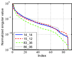
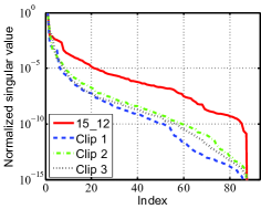
Figure 2: The vertical axis is the normalized singular value and the horizontal axis is its index. (a) As the normalized singular values approach zero quickly, matrix $\bf M$ is of low rank and its rows are strongly dependent. (b) We randomly extract three clips from a sequence. Each clip has 300 frames. The singular values of the clips approach zero more quickly than that of the whole sequence, indicating that short clips have stronger inter-correlation than the whole sequence.

III-B Local v.s. Global

Motion in a short period tends to be more correlated than in a long period, indicating that short clips have stronger inter-correlation than the whole sequence.

To verify the local property, we randomly extract several clips from a sequence. Each clip has $F(\ll f)$ frames and is represented by a matrix $\overline{\mathbf{M}}\in\mathbb{R}^{3n\times F}$. Then, we compare their normalized singular values with those of the big matrix $\mathbf{M}$. Fig. 2 shows that the singular values of $\overline{\mathbf{M}}$ approach to zero more rapidly than $\mathbf{M}$, meaning that the clips have stronger inter-correlation than the whole sequence $\mathbf{M}$.

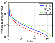
(a) Mocap data

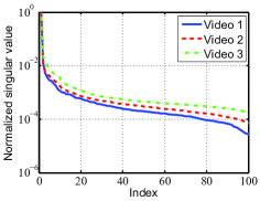
(b) Natural videos

Figure 3: The normalized singular values of an unfolded mocap matrix approaches zero faster than natural videos. The three natural videos, CREW, SOCCER, and BUS, are from the standard video compression test sequences [Online] Available: http://trace.eas.asu.edu/yuv/.

III-C Clip Correlation

Intuitive speaking, a long motion sequence (such as walking, jogging, etc) has repeated motions. Thus, one clip or several markers’ trajectories can be obtained by blending others. Such a property is more obvious in large mocap database.

Similar to [18], we verify the clip correlation by partitioning $\mathbf{M}$ into $J$ non-overlapping clips represent them as a three dimensional matrix $\mathcal{M}\in\mathbb{R}^{3n\times f/J\times J}$. A new matrix $\mathbf{\widetilde{M}}\in\mathbb{R}^{J\times 3nf/J}$ is formed by unfolding the matrices $\mathcal{M}$ along the third dimension. We then factorize $\widetilde{\mathbf{M}}$ by SVD. Fig. 3(a) shows that the normalized singular values of $\widetilde{\mathbf{M}}$ of all test mocap data approach zero rapidly, indicating that mocap clips have strong correlation. We also perform the test on natural videos, in which a clip is one video frame. As shown in Fig. 3(b), the clip correlation in natural videos is not as strong as the mocap data.

IV Our Algorithm

IV-A Motivation

As mentioned above, a key issue of compressing mocap data is to reduce data correlation described in Section III-A, as much as possible. A straightforward method is to directly apply 2D transform coding to $\bf M$. However, our analysis in Section III-B suggests that compressing subsequences separately is more effective than that of the sequence as a whole. Similar observation can be found in [1], [6], [9] and image/video compression, where block-based transform is widely used. Moreover, processing each clip separately is obviously more memory efficient than that of the whole sequence. Inspired by these observations, we propose a clip-based algorithm for compressing mocap data, in which one mocap sequences is segmented into $N$ clips, and the $i$-th clip is denoted by $\mathbf{M}_{i}\in\mathbb{R}^{3n\times L_{i}}$ with $L_{i}$ stands for the length.

Within the transform coding framework, one needs to transform the input data into the transform domain, in which the transformed coefficients exhibit sparsity so that some smallest ones can be discarded with little information loss. A possible solution is to apply SVD to each $\mathbf{M}_{i}$ and then keep the top $k_{i}$ important components, i.e.,

$$\left[\mathbf{U}_{1}^{\intercal}\mathbf{M}_{1}\mathbf{V}_{1}~{}~{}\mathbf{U}_{2}^{\intercal}\mathbf{M}_{2}\mathbf{V}_{2}~{}~{}\cdots~{}~{}\mathbf{U}_{N}^{\intercal}\mathbf{M}_{N}\mathbf{V}_{N}\right]$$

$$=\left[\overline{\mathbf{S}}_{1}~{}~{}\overline{\mathbf{S}}_{2}~{}~{}\cdots~{}~{}\overline{\mathbf{S}}_{N}\right],$$ (1)

where $\mathbf{U}_{i}\in\mathbb{R}^{3n\times k_{i}}$ and $\mathbf{V}_{i}\in\mathbb{R}^{L_{i}\times k_{i}}$ are the $k_{i}$ eigenvectors of $\mathbf{M}_{i}\mathbf{M}_{i}^{\intercal}$ and $\mathbf{M}_{i}^{\intercal}\mathbf{M}_{i}$, corresponding to the $k_{i}$ largest eigenvalues, respectively, and $\overline{\mathbf{S}}_{i}\in\mathbb{R}^{k_{i}\times k_{i}}$ is a diagonal matrix. The SVD-based transform coding uses knowledge of the application to choose information to discard. However, since one has to store all the transformation matrices $\mathbf{U}_{i}$ and $\mathbf{V}_{i}$, $i=1,\cdots,N$, it is difficult to obtain high compression performance.

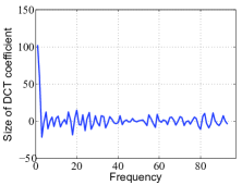
(a) Human motion

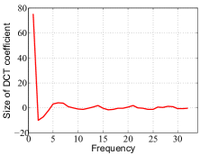
(b) Natural image

Figure 4: Applying the 1D DCT to the columns of a natural image, we can see sparsity in the transform domain. However, human motion data do not have such a property due to lack of smoothness in the column direction.

Alternatively, one may adopt some application-independent transformations, such as 2D DCT or DWT. Take 2D DCT as an example.

$$\mathbf{D}_{l}^{\intercal}[\mathbf{M}_{1}\mathbf{D}_{r_{1}}~{}~{}\mathbf{M}_{2}\mathbf{D}_{r_{2}}~{}~{}\cdots~{}~{}\mathbf{M}_{N}\mathbf{D}_{r_{N}}]$$

$$=\left[\widetilde{\mathbf{S}}_{1}~{}~{}\widetilde{\mathbf{S}}_{2}~{}~{}\cdots~{}~{}\widetilde{\mathbf{S}}_{N}\right],$$ (2)

where $\mathbf{D}_{l}\in\mathbb{R}^{3n\times 3n}$ and $\mathbf{D}_{r_{i}}\in\mathbb{R}^{L_{i}\times L_{i}}$ are the standard 1D DCT basis matrices, $\widetilde{\mathbf{S}}_{i}\in\mathbb{R}^{3n\times L_{i}}$ are the transformed coefficients. Compared to the SVD-based transform coding, the DCT-based approach stores only the transformed matrices $\widetilde{\mathbf{S}}_{i}$, $i=1,\cdots,N$. Owning to the locally smooth (or small variation) nature of images, the DCT works extremely well in 2D image and video compression.

  Figure 5: Applying the DCT to $\mathbf{M}_{i}$’s rows, we see sparsity in the transform domain. However, as discussed above, the columns in mocap data are not smooth. Therefore, it does not make sense to apply the left transform $\mathbf{D}_{l}$ to mocap data. Fig. 4(a) reveals such an issue by applying the 1D DCT to a randomly-chosen column in $\mathbf{M}_{i}$. We can clearly see that the transform coefficients occupy a wide range of frequencies. In sharp contrast, applying the 1D DCT to an arbitrary natural image column produces very small range of frequencies in the transformed coefficients. See Fig. 4(b). On the other hand, rows of a mocap matrix are smooth since each marker has a smooth trajectory. Applying the 1D DCT to an arbitrary row of $\mathbf{M}_{i}$ shows that the DCT coefficients occupy only a small range. See Fig. IV-A.

Motivated by the above discussions and observations, to develop an effective compression method for mocap sequences, one must take knowledge of mocap data into account and also keep the number of transform matrices as small as possible. Towards this goal, we propose a novel mocap tailored transform coding method. As shown in Fig. 6, after segmentation, we compute the data-dependent transformation matrix $\mathbf{B}\in\mathbb{R}^{3n\times k}$,

$$\mathbf{B}^{\intercal}\left[\mathbf{M}_{1}\widetilde{\mathbf{D}}_{r_{1}}~{}~{}\mathbf{M}_{2}\widetilde{\mathbf{D}}_{r_{2}}~{}~{}\cdots~{}~{}\mathbf{M}_{N}\widetilde{\mathbf{D}}_{r_{N}}\right]$$

$$=[\mathbf{S}_{1}~{}~{}\mathbf{S}_{2}~{}~{}\cdots~{}~{}\mathbf{S}_{N}],$$ (3)

which can reveal the geometric structure of columns of $\mathbf{M}_{i}$ to lead correlation removal, where $\widetilde{\mathbf{D}}_{r_{i}}\in\mathbb{R}^{L_{i}\times l_{i}}$ is the truncated 1D DCT transform matrix and $\mathbf{S}_{i}\in\mathbb{R}^{k\times l_{i}}$ is dense coefficients.

It is worth noting that our method is able to adopt a single data-dependent left transform due to the strong correlation among mocap clips described in Section III-C. Our mocap tailored transform coding stores only $k\left(3n+\sum_{i=1}^{N}l_{i}\right)$ scalars in the transform domain, whereas the SVD-based method (see Eqn. (1)) requires $3n\sum_{i=1}^{N}k_{i}+\sum_{i=1}^{N}(L_{i}l_{i}+k_{i})$ scalars.

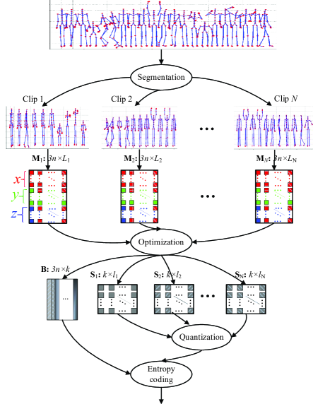
Figure 6: The flow chart of our algorithm.

IV-B Mocap Tailored Transform Coding

Computing the data-tailored transform matrix $\mathbf{B}$ and coefficient matrices $\mathbf{S}_{i}$ is formulated as a least-square problem:

$$\min_{\mathbf{B},\mathbf{S}_{i}}\sum_{i=1}^{N}\left\|\mathbf{M}_{i}-\mathbf{B}\mathbf{S}_{i}\widetilde{\mathbf{D}}_{r_{i}}^{\intercal}\right\|_{F}^{2}$$

$$~{}~{}~{}~{}~{}s.t.~{}~{}~{}\mathbf{B}^{\intercal}\mathbf{B}=\mathbf{I}_{k},$$ (4)

where $\|\cdot\|_{F}$ is the Frobenius norm defined as $\|\mathbf{X}\|_{F}=\sqrt{\sum_{i}\sum_{j}X_{i,j}^{2}}$, and $\mathbf{I}_{k}\in\mathbb{R}^{k\times k}$ is the identity matrix. To minimize (4), the partial deviation of (4) with respect to $\mathbf{S}_{i}$ must be equal to zero. So we obtain $\mathbf{S}_{i}$ must satisfy $\mathbf{S}_{i}=\mathbf{B}^{\intercal}\mathbf{M}_{i}\widetilde{\mathbf{D}}_{r_{i}}$. With $\|\mathbf{X}\|_{F}^{2}={\rm Tr}(\mathbf{X}\mathbf{X}^{T})$ where Tr is for the trace of matrix, i.e., ${\rm Tr}(\mathbf{X})=\sum_{i}X_{i,i}$, we can rewrite the objective function as

$$\sum_{i=1}^{N}\left\|\mathbf{M}_{i}-\mathbf{B}\mathbf{S}_{i}\widetilde{\mathbf{D}}_{r_{i}}^{\intercal}\right\|_{F}^{2}$$

$$=\sum_{i=1}^{N}\left\{{\rm Tr}\left(\mathbf{M}_{i}\mathbf{M}_{i}^{\intercal}\right)+{\rm Tr}\left(\mathbf{S}_{i}\mathbf{S}_{i}^{\intercal}\right)-2{\rm Tr}\left(\mathbf{B}\mathbf{S}_{i}\widetilde{\mathbf{D}}_{r_{i}}^{\intercal}\mathbf{M}_{i}^{\intercal}\right)\right\}$$

$$=\sum_{i=1}^{N}\left\{{\rm Tr}\left(\mathbf{M}_{i}\mathbf{M}_{i}^{\intercal}\right)+{\rm Tr}\left(\mathbf{B}^{\intercal}\mathbf{M}_{i}\widetilde{\mathbf{D}}_{r_{i}}\widetilde{\mathbf{D}}_{r_{i}}^{\intercal}\mathbf{M}_{i}^{\intercal}\mathbf{B}\right)\right.$$

$$\left.-2{\rm Tr}\left(\mathbf{B}\mathbf{B}^{\intercal}\mathbf{M}_{i}\widetilde{\mathbf{D}}_{r_{i}}\widetilde{\mathbf{D}}_{r_{i}}^{\intercal}\mathbf{M}_{i}^{\intercal}\right)\right\}$$

$$=\sum_{i=1}^{N}{\rm Tr}\left(\mathbf{M}_{i}\mathbf{M}_{i}^{\intercal}\right)-{\rm Tr}\left(\mathbf{B}^{\intercal}\mathbf{C}\mathbf{B}\right),$$ (5)

where $\mathbf{C}=\sum_{i=1}^{N}\mathbf{M}_{i}\widetilde{\mathbf{D}}_{r_{i}}\widetilde{\mathbf{D}}_{r_{i}}^{\intercal}\mathbf{M}_{i}^{\intercal}$. The last equation comes from the fact $\mathrm{Tr}(\mathbf{X}\mathbf{Y})=\mathrm{Tr}(\mathbf{Y}\mathbf{X})$ for compatible matrices $\mathbf{X}$ and $\mathbf{Y}$.

The first term in Eqn. (5) is a constant, which is independent of $\mathbf{B}$. Therefore, the minimization problem in (4) is equivalent to the following maximization problem, i.e.,

$$\max_{\mathbf{B}}~{}{\rm Tr}\left(\mathbf{B}^{\intercal}\mathbf{C}\mathbf{B}\right)$$

$$~{}~{}~{}s.t.~{}~{}~{}\mathbf{B}^{\intercal}\mathbf{B}=\mathbf{I}_{k}.$$ (6)

The optimal solution of (6) is given in Theorem 1.

It takes $\mathcal{O}\left(nN\max_{i}\{l_{i}\}(\max_{i}\{L_{i}\}+n)\right)$ time to compute the matrix $\mathbf{C}$. We adopt the SVD algorithm for solving $\mathbf{C}$’s eigen system, which takes $\mathcal{O}(n^{3})$ time. Finally, computing all $\mathbf{S}_{i}$ takes $\mathcal{O}(nN\max_{i}\{l_{i}\}(\max_{i}\{L_{i}\}+k))$ time. Since the number of markers $n$ is usually small (e.g., a few tens), the dominating term in the time complexity is $\mathcal{O}(nN\max_{i}\{l_{i}\}(\max_{i}\{L_{i}\}+n+k))$.

Theorem 1 ([19])

Given a symmetric matrix $\mathbf{X}$ of dimension $p\times p$ and an arbitrary orthogonal matrix Y of dimension $p\times q$, the trace of $\mathbf{Y}^{T}\mathbf{X}\mathbf{Y}$ is maximized when $\mathbf{Y}$ contains the $q$ eigenvectors of $\mathbf{X}$, which correspond to the $q$ (algebraically) largest eigenvalues.

IV-C Quantization and Entropy Coding

Since the compression quality highly depends on the accuracy of the orthogonal matrix $\mathbf{B}$, we represent each element of $\mathbf{B}$ using 16 bits. For each element of $\mathbf{S}_{i}$, we quantize its fractional part with $Q_{i}$ bits per entry, where $Q_{i}$ is automatically determined by our algorithm (see Section VI-A). Then we adopt the lossless coding scheme to encode the bitstream. Note that other advanced lossless entropy coding schemes can also be applied. The decoder is a straightforward process that computes decompressed clip by $\widehat{\mathbf{B}}\mathbf{\widehat{S}}_{i}\mathbf{D}_{r_{i}}^{\intercal}$, where $\mathbf{\widehat{B}}$ and $\mathbf{\widehat{S}}_{i}$ are the decoded matrices.

V Generalization to Mocap Database

The previous section presents our algorithm for compressing a single human motion sequence. In this section, we consider a general scenario of human mocap database, which may consist of a large amount of motion sequences recorded from multiple performers. Due to diversity, a single transformation matrix $\mathbf{B}$ may not work for all clips. Therefore, it is natural to consider multiple transformation matrices to improve the compression result. We formulate the problem as computing $K$ transform matrices $\mathbf{B}_{j}$, $j=1,\cdots,K$, so that all clips can be selectively projected on them with the least distortion

$$\min_{\mathbf{W},\{\mathbf{B}_{j}\}_{j=1}^{K}}\sum_{i=1}^{N}\sum_{j=1}^{K}W_{i,j}\left\|\mathbf{M}_{i}-\mathbf{B}_{j}\mathbf{S}_{i,j}\widetilde{\mathbf{D}}_{r_{i}}^{\intercal}\right\|_{F}^{2},$$

$$s.t.~{}\forall j,~{}\mathbf{B}_{j}^{\intercal}\mathbf{B}_{j}=\mathbf{I}_{k},$$

$$~{}~{}~{}~{}~{}\forall i,j,~{}W_{i,j}\in[0,1],$$

$$~{}~{}~{}~{}~{}\forall i,\sum_{j=1}^{K}W_{i,j}=1,$$ (7)

where $W_{i,j}$ is the $(i,j)$-th entry of $\mathbf{W}$ indicating whether the $i$-th clip is represented in the space spanned by the $j$-th transform matrix $\mathbf{B}_{j}$. Obviously, Eqn. (4) is a special case of Eqn. (7) with $K=1$.

Note that the optimization problem (7) is not easy to solve due to the two types of variables involved. In this paper, we propose a deterministic annealing based method [20] that iteratively solves only one variable ($\mathbf{B}_{j}$ or $W_{ij}$) at a time. In each iteration, we first update $\mathbf{S}_{i,j}$ with other variables fixed

$$\centering\mathbf{S}_{i,j}=\mathbf{B}_{j}^{\intercal}\mathbf{M}_{i}\widetilde{\mathbf{D}}_{r_{i}}.\@add@centering$$ (8)

Then we update $W_{i,j}$ using the centroid equation,

$$\centering W_{i,j}=\frac{e^{-\frac{1}{t}\left\|\mathbf{M}_{i}-\mathbf{B}_{j}\mathbf{S}_{i,j}\widetilde{\mathbf{D}}_{r_{i}}^{\intercal}\right\|_{F}^{2}}}{\sum_{h=1}^{K}e^{-\frac{1}{t}\left\|\mathbf{M}_{i}-\mathbf{B}_{l}\mathbf{S}_{i,h}\widetilde{\mathbf{D}}_{r_{i}}^{\intercal}\right\|_{F}^{2}}},\@add@centering$$ (9)

where $t$ is the temperature. By cooling the temperature slowly, the global optimal solution is obtained [20]. Next, we compute matrix $\mathbf{C}_{j}$

$$\centering\mathbf{C}_{j}=\sum_{i=1}^{N}W_{i,j}\mathbf{M}_{i}\widetilde{\mathbf{D}}_{r_{i}}\widetilde{\mathbf{D}}_{r_{i}}^{\intercal}\mathbf{M}_{i}^{\intercal},\@add@centering$$ (10)

and solve its eigensystem using SVD. Finally, we form matrix $\mathbf{B}_{j}$ by taking $\mathbf{C}_{j}$’s $k$ eigenvectors associated with the largest $k$ eigenvalues. We repeat the above procedures until convergence, i.e., the change of matrices $\mathbf{B}_{j}$ and $\mathbf{W}$ is less than a small tolerance . The above deterministic simulated annealing method is guaranteed to converge [20]. Computational results show that it usually converges in less than 30 iterations given a tolerance of $10^{-6}$.

Algorithm 1 Deterministic annealing based alternating iteration algorithm for solving (7).

Input: $\{\mathbf{M}_{i}\}_{i=1}^{N}$, $K$
Output: $\{\mathbf{B}_{j}\}_{j=1}^{K}$ and $\mathbf{W}$
Initialization: initialize $\mathbf{B}_{j}$ with random orthogonal bases and $\widetilde{\mathbf{D}}_{r_{i}}$ with DCT bases; set $W_{i,j}=1/K$ and $t>0$.

1:  repeat

2:     for $i\leftarrow 1:N$ do

3:        for $j\leftarrow 1:K$ do

4:           $\mathbf{S}_{i,j}=\mathbf{B}_{j}^{\intercal}\mathbf{M}_{i}\widetilde{\mathbf{D}}_{r_{i}}$

5:        end for

6:        for $j\leftarrow 1:K$ do

7:           compute $W_{i,j}$ using (9)

8:        end for

9:     end for

10:     for $j\leftarrow 1:K$ do

11:        compute $\mathbf{C}_{j}$ using (10)

12:        $\mathbf{B}_{j}\leftarrow$ $\mathbf{C}_{j}$’s $k$ eigenvectors associated with the $k$ largest eigenvalues

13:     end for

14:     $t\leftarrow\frac{t}{2}$

15:  until convergence

VI Experimental Results and Discussion

TABLE II: The test data is from CMU Mocap database [35], where each motion sequence has 31 markers and with a frame rate 120 fps.

Sequences	# of frames	Size (MB)	Description
Used in Section III
14_14	4,653	1.65	jumping, jog, squats, side twists, stretches
15_12	9,086	3.22	wash windows, lay-up shot, pass, throw ball, dance, the dive, the twist, strew
38_04	8,631	3.06	walk around, frequent turns, cyclic walk along a line
83_36	1,062	0.38	walk turn 90 degrees left walk forward
86_06	9939	3.63	walking, running, kicking, punching, knee kicking, and stretching
Used in Section VI-A
86_02	10617	3.77	walk, squats, run, stretch, jumps, punches, and drinking
86_12	8,856	3.14	walking, dragging, sweeping, dustpan, wipe window, and wipe mirror
Used in Section VI-B
41_07	7,536	2.67	climb, step over, jump over, navigate around stepstool
56_07	9,420	3.34	yawn, stretch, walk, run/jog, angrily grab, jump, skip, halt
69_08	5,309	1.88	walk and turn
86_05	8,340	2.96	walking, jumping, jumping jacks, jumping on one foot, punching
database_1	291,506	103.41	all sequences of subject: 31, 40 and 86
database_2	223,852	79.41	all sequences of subject: 105, 106, 111 and 113
Used in Section VI-C
15_04	22,549	8.02	wash windows, paint, hand signals, dance, the dive, the twist, boxing
17_08	6,197	2.20	muscular, heavyset person’s walk
17_10	2,783	0.99	boxing
85_12	4,499	1.60	jumps, flips, breakdance
database_3	341,472	121.14	all sequences of subject: 6, 15, 16, 17, 35, 94 and 135
database_4	122,846	43.58	all sequences of subject: 1, 2, 5, 6, 9, and 12

VI-A Parameter Setting

The performance of our algorithm depends on the clip lengths $L_{i}$, $i=1,2,\cdots,N$, which are specified by either the user or a motion segmentation algorithm, and three parameters, i.e., $k$, $l_{i}$, and $Q_{i}$, which are determined by our algorithm automatically. For database, the user also specifies the number of transform matrices $K$.

Throughout this paper, the compression ratio (CR) is defined as the ratio of the original data size to the compressed data size. We measure the distortion using average Euclidian distance (in cm), i.e.,

$$\centering\overline{d}=\frac{1}{nf}\sum_{i=1}^{n}\sum_{j=1}^{f}\sqrt{\left(\mathbf{p}_{i,j}-\widehat{\mathbf{p}}_{i,j}\right)\left(\mathbf{p}_{i,j}-\widehat{\mathbf{p}}_{i,j}\right)^{\intercal}},\@add@centering$$ (11)

where $\mathbf{p}_{i,j}=[x_{i,j}~{}y_{i,j}~{}z_{i,j}]$ and $\widehat{\mathbf{p}}_{i,j}=[\widehat{x}_{i,j}~{}\widehat{y}_{i,j}~{}\widehat{z}_{i,j}]$ are original and decompressed 3D coordinates of the $i$-th marker in the $j$-th frame, respectively.

Here, we show how the parameters $k$, $l_{i}$, and $Q_{i}$ are automatically set in our scheme. To simplify the analysis, we simply take all clips equally, i.e., $L_{i}\equiv L$, $l_{i}\equiv l$ and $Q_{i}\equiv Q$ for all $i$. The parameters $k$ and $l$ specify the number of retained important coefficients in transform coding. Taking more coefficients in the direction with weaker correlation can effectively reduce the distortion and improve the compression performance. The degree of correlation within each row of $\mathbf{M}_{i}$ depends on the clip lengths, and computational results show that the ratio $r=l/k$ that leads to the least distortion is linearly proportional to clip length $L$ and we adopt the following empirical formula:

$$\centering r=0.1\times\left\lceil\frac{L}{50}\right\rceil,\@add@centering$$ (12)

where $\lceil\cdot\rceil$ is the ceiling function. See Fig. 7.

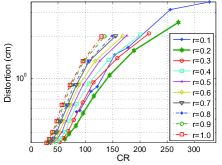
(a) $L$=70

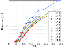
(b) $L$=130

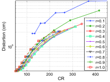
(c) $L$=180

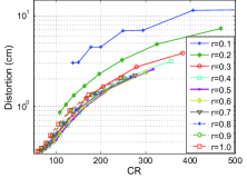
(d) $L$=240

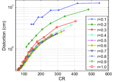
(e) $L$=280

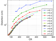
(f) $L$=340

Figure 7: The impact of the ratio $r=l/k$ on compression performance under various clip lengths on the test sequence 86_02. In each figure, the thick line is the optimal result.

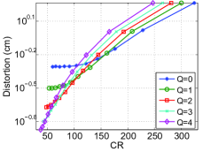
(a) Sequence 15_12

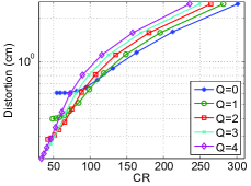
(b) Sequence 38_04

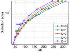
(c) Sequence 55_28

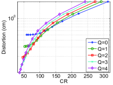
(d) Sequence 86_12

Figure 8: Compression performance and the quantization parameter $Q$. In each curve plot, the parameter $k$ is sampled from $15$ to $65$ with a step length $5$. The clip length $L=270$.

The quantization parameter $Q$ determines the size of the fractional parts of the transformed coefficients. Increasing $Q$ leads to more accurate results, but it reduces the compression ratio. Fig. 8 shows that smaller $Q$ produces better results at high CRs and larger $Q$ is preferred at low CRs. In our implementation, we adopt the following empirical formula:

$$\centering Q=\left\{\begin{array}[]{ccc}0&0<k\leq 30\\ \\ \left\lceil\frac{k-30}{10}\right\rceil&30<k\leq 93.\end{array}\right.\@add@centering$$ (13)

VI-B Results

We implement our algorithm in MATLAB and evaluate its performance and quality on the CMU Mocap Database [35]. Table II shows the details of the test data. We use the MATLAB toolbox [36] to decode the .asf/.amc into 3-D marker coordinates, which are stored as 32-bit floating-points.

We test our method under two scenarios, i.e., equal segmentation and adaptive segmentation. Various CRs are obtained by changing the parameter $k$.

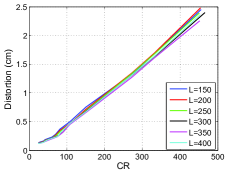
(a) Sequence 41_07

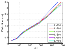
(b) Sequence 56_07

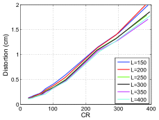
(c) Sequence 69_08

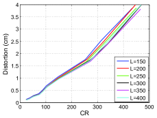
(d) Sequence 86_05

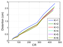
(e) database_1 ($L$=280)

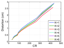
(f) database_2 ($L$=280)

Figure 9: CR-distortion curves for equal segmentation.

TABLE III: Algorithm efficiency. $E_{fps}$ and $D_{fps}$ are the encoding and decoding frame rates, respectively.

Data	15_04	17_08	17_10	85_12	41_07	56_07	69_08	86_05	database_1	database_2
$E_{fps}(\times 10^{4})$	17.2	7.19	3.24	4.90	7.88	9.61	5.98	8.64	0.23	0.21
$D_{fps}(\times 10^{4})$	27.6	9.65	4.18	6.83	10.9	13.5	7.92	12.1	34.6	31.4

VI-B1 Equal segmentation

In this scenario, we segment mocap data into clips with equal length, i.e., $L_{1}=L_{2}=\cdots=L_{N}=L$. Equal segmentation is easy to implement and it is often used when $L$ is specified by the user, since it is tedious for the user to specify the length for each clip separately.

First, we test our method on mocap sequences by setting various $L$s. We observe that increasing $L$ can improve the compression performance, but the improvement becomes less significant when $L\geq 350$. As Figs. 9 and 10 show, the distortion is less than 1cm when CR$\geq 100$. See also the accompanying video for more results.

Then, we apply our method to mocap databases. We specify one more parameter $K$ for the number of transform matrices. Intuitively, the more the data-dependent transform matrices, the less the distortion. However, since the orthogonal matrices $\mathbf{B}_{i}$ are difficult to compress, more spaces are required to store them, which reduces the compression ratio. Fig. 9 shows that we achieve the optimal compression performance for database_1 and database_2 when $K$ is equal to 4 and 3, respectively.

Table III shows the performance statistics of our method. Our unoptimized and serial MATLAB code is able to encode more than 10,000 frames per second for a single mocap sequence. It can also encode 2,000 fps for mocap databases. The decoding speed is even faster than encoding. It is worth noting that our method can be further sped up by parallel computation. For example, computing $\mathbf{S}_{i}$ can be implemented in parallel on the GPUs.

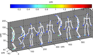
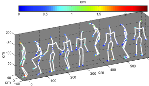
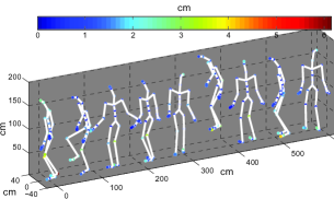
CR=97.9CR=146.8CR=281.3
(a) Sequence 41_07
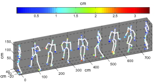
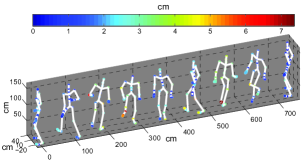
CR=86.9CR=148.6CR=289.9
(b) Sequence 56_07
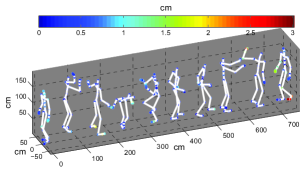
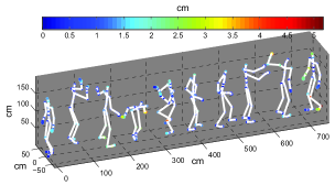
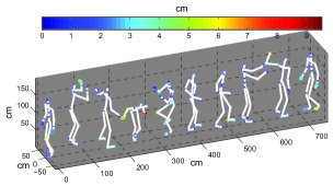
CR=79.1CR=142.5CR=271.9
(c) Sequence 86_05

Figure 10: Visual results for equal clip segmentation ($L$=280). The joint distortions are colored in heatmap.

To demonstrate the robustness of our method, we also test our method on sequences with low frame rates, which have weaker data correlation than the ones at full frame rates. Given the original sequences with 120 fps, we uniformly downsampled them to 60 fps. Correspondingly, their data size and number of frames halved. As Fig. 11 shows, our method still works very well, i.e., under the same distortion, the CRs is approximate 50% of those in Fig. 9. We also observe that the optimal range $L\in[150,200]$ is approximately half of the one in Fig. 9.

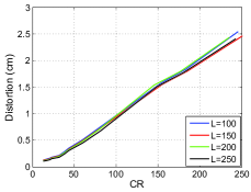
(a) Sequence 41_07

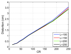
(b) Sequence 56_07

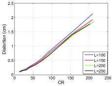
(c) Sequence 69_08

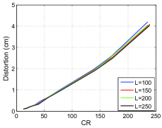
(d) Sequence 86_05

Figure 11: Our results are not sensitive the frame rate. The original test data were obtained at 120 fps and we downsampled each sequence to 60fps and segmented them into clips of equal length. With doubled compression ratio, the distortion curves are similar to Figure 9.

VI-B2 Adaptive segmentation

When advanced motion analysis tool (e.g., [25], [23], [24], [28]) is available, one can segment the input data to clips of physically meaningful actions, which have stronger correlation than fixed-length clips. In our implementation, we adopt the probabilistic principal component analysis (PPCA)-based segmentation algorithm [25] for its simplicity and effectiveness, in which a cut is made when the distribution of human poses changes. Other advanced and complicated motion segmentation algorithms, e.g., [23] and [28], can also be employed. The parameters of the $i$-th clip, i.e., $l_{i}$ and $Q_{i}$, are obtained by Eqns. (12) and (13) according to the clip length $L_{i}$. We also set various numbers of clips during the segmentation to investigate how it affects the compression performance. As shown in Fig. 12, the optimal number of clips (or segments) depend on the motion characteristics. For example, the sequence 69_08 contains only walking and turning, so a small number of clips works well. In contrast, the sequences 56_07 and 86_05 contain complicated motions, such as climbing punching. As a result, a large number of clips produces smaller distortion. As expected, at relatively high CRs, adaptive segmentation can achieve higher compression performance than equal segmentation.

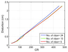
(a) Sequence 41_07

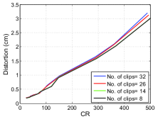
(b) Sequence 56_07

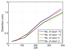
(c) Sequence 69_08

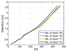
(d) Sequence 86_05

Figure 12: CR-distortion curves for adaptive segmentation with various clip numbers.

VI-C Comparison

We compare our method with several state-of-the-art techniques [6], [10], [11], [12], [13] in terms of compression performance and efficiency. The results of [6], [10], and  [11] are taken from [11], and the results of [12] and [13] are taken from [13]. Note that only results with a single compression ratio were provided in both [11] and [13]. For fair comparison, our scheme is performed under the equal segmentation scenario. Fig. 13 shows our CR-distortion curves on some test sequences and mocap databases. We observe that our CR-distortion curves are consistently below the other methods, indicating that our method outperforms them in terms of compression performance. Table IV shows that our method is also much more efficient than the existing methods.

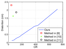
(a) Sequence 15_04

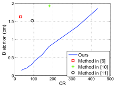
(b) Sequence 17_08

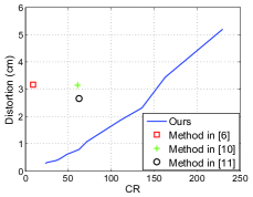
(c) Sequence 17_10

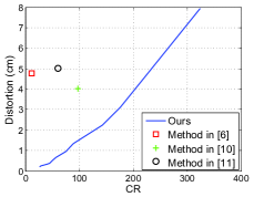
(d) Sequence 85_12

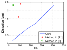
(e) database_3

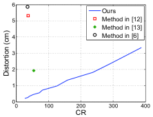
(f) database_4

Figure 13: Comparison in terms of compression performance. Our method is performed under equal segmentation with $L=280$. In (a), (b), (c) and (d), the results of [6], [10], [11] are taken from [11], where only a single CR was provided. For database_3, $K=4$ and the results of [11] and [6] are taken from [11]. For database_4, $K=3$ and the results of [6], [12] and [13] are taken from [13].

TABLE IV: Efficiency comparison. The results of Arikan [6] and Lin et al. [11] are taken from [11], which were measured on an Intel 3.0GHz CPU. We evaluated our algorithm on an Intel 3.1GHz CPU. Computational results show that our method is significantly faster than the existing methods and also produces results of better quality. $\overline{d}$ is the distortion (in cm), $E_{fps}$ and $D_{fps}$ are the encoding and decoding frame rates, respectively.

	Arikan [6]				Ours				Lin et al [11]				Ours
Seq.	CR	$\overline{d}$	$E_{fps}$	$D_{fps}$	CR	$\overline{d}$	$E_{fps}$	$D_{fps}$	CR	$\overline{d}$	$E_{fps}$	$D_{fps}$	CR	$\overline{d}$	$E_{fps}$	$D_{fps}$
15_04	42.5	2.30	705.6	2693.7	45.7	0.12	125,934	261,563	114.7	1.86	219.1	2530.8	114.1	0.29	169,567	281,478
17_08	30.0	1.63	778.8	2979.8	35.0	0.15	58,576	88,967	91.2	1.52	539.1	2945.2	93.8	0.37	69,856	91,729
17_10	9.2	3.16	376.7	4596.8	14.2	0.22	27,748	39,254	62.6	2.65	486.6	4288.1	63.2	1.07	32,348	40,239
85_12	11.1	4.78	585.7	3903.1	16.1	0.12	43,173	69,187	60.1	5.01	506.4	3096.4	59.3	0.84	52,269	68,546
database_3	39.8	2.32	530.5	4902.3	40.6	0.20	1,805	294,536	88.7	1.60	372.4	4286.8	83.7	0.47	1,798	293,947

VI-D Limitation

The high compression performance of our method comes by significantly exploring the temporal correlation, that is, it requires the entire sequence or at least a sequence of sufficiently long period to compute the left transform matrix using Eq. (4). This will cause the latency problem, which also occurs in other approaches, e.g., [1, 6, 9, 21, 11]. Thus, it is not suitable for applications where data acquisition and compression have to be done simultaneously or within a very small time interval.

VII Conclusion and Discussion

This paper has presented a mocap-tailored transform coding for compressing human mocap data. Our method is highly effective in that it takes advantage of the features of mocap data. Furthermore, it has low computational cost and can be easily extended to compress mocap databases. Unlike existing approaches, it requires neither training nor complicated parameter setting. Experimental results demonstrate that the proposed scheme significantly outperforms state-of-the-art algorithms in terms of compression performance and speed.

Owning to its high performance, we believe our method has potential to many mocap applications, such as retrieval [26, 27, 29, 30], where the clip dimensionality can be significantly reduced without comprising data quality, leading to low computational complexity. Besides mocap data, our method can be extended for compressing dynamic meshes [31, 32], in which each vertex is considered as a marker.

Our method can also inspire interesting future work.

1. We observed that the compression performance depends on the compressed transform matrices. Therefore, advanced matrix compression algorithms, e.g., sparse and redundancy representation, can improve our results.

2. Perception-based compression schemes [33, 34] have proven to be effective to natural images and videos, since they are adaptive to human vision system. It would be interesting to investigate the perceived-based methods for mocap data compression. For example, optimally allocating bits to clips guided by a perceptual distortion metric, that is, clips which can be significantly compressed with little perceptual distortion should be assigned fewer bits, and vice versa, so that the overall compression performance is higher.

3. In our implementation, we focus on human motion capture data. It is also interesting to check its performance on other types of mocap data, e.g., facial expressions.

4. A possible solution to solve the latency problem is to apply machine learning techniques to pre-compute some left transform matrices from learning datasets. As a result, the compression can be carried out whenever a clip with small length is available.

5. Last but not least, it is desirable to develop a fully automatic algorithm for determining the optimal (or near-optimal) parameter, i.e., the clip lengths for equal segmentation and the number of clips for adaptive segmentation.

References

- [1] G. Liu and L. McMillan, “Segment-based human motion compression,” Proc. ACM SIGGRAPH/Eurographics Symposium on Computer Animation, pp. 127-135, 2006.
- [2] S. Chattopadhyay, S. M. Bhandarkar, and K. Li, “Human motion capture data compression by model-based indexing: a power aware approach,” IEEE Trans. Visualization and Computer Graphics, vol. 13 ,no. 1, pp. 5-14, 2007.
- [3] P. Beaudoin, P. Poulin, and Michiel van de Panne, “Adapting wavelet compression to human motion capture clips,” Proc. Graphics Interface, pp. 313-318, 2007.
- [4] I.S. Lim and D. Thalmann, “Key posture extraction out of human motion data by curve simplification”, 23rd Annual International Conference IEEE Engineering in Medicine and Biology Society 2001, pp. 1167-1169, 2001.
- [5] J. Xiao, Y. Zhuang, T. Yang, and F. Wu, “An efficient keyframe extraction from motion capture data,” Proc. Computer Graphics International Conference, pp. 494-501, 2006.
- [6] O. Arikan, “Compression of Motion Capture database,” ACM Trans. on Graphics, vol. 25, no. 3, pp. 890-897, 2006.
- [7] M.-H Kim, L.-P Chau, and W.-C. Siu, “Keyframe selection for motion capture using motion activity analysis,” in Proc. IEEE International Symposium on Circuits and Systems, pp. 612-615, 2012.
- [8] Y. Li, C. Fermuller, Y. Aloimonos, and H. Ji, “Learning shift-invariant sparse representation of actions,” in Proc. IEEE Conference on Computer Vision and Pattern Recognition, pp. 2630-2637, 2010.
- [9] B.-S. Chew, L.-P. Chau, K.-H. Yap, “A fuzzy clustering algorithm for virtual character animation representation,” IEEE Trans. Multimedia, vol. 13, no. 1, pp. 40-49, 2011.
- [10] M. Tournier, X. Wu, N. Courty, E. Arnaud, and L. Reveret, “Motion compression using principal geodesics analysis,” Computer Graphics Forum, vol. 28, no. 2, pp. 355-364, 2009.
- [11] I-C. Lin, J.-Y. Peng, C.-C. Lin, and M.-H. Tsai, “Adaptive motion data representaion with repeated motion analysis,” IEEE Trans. Visualization and Computer Graphics, vol. 17, no. 4, pp. 527-538, 2011.
- [12] Q. Gu, J. Peng, and Z. Deng, “Compression of human motion capture data using motion pattern indexing,” Computer Graphics Forum, vol. 28, no. 1, pp. 1-12, 2009.
- [13] M. Zhu, H. Sun, Z. Deng, “Quaternion space sparse decomposition for motion compression and retrieval,” Proc. ACM SIGGRAPH/Eurographics Symposium on Computer Animation, pp. 183-192, 2012.
- [14] L. Ren, “Statistical analysis of natural human motion for animation,” Ph.D. dissertation, Pittsburgh, PA, USA, 2006.
- [15] M. Preda and F. Preteux, “Virtual character within MPEG-4 animation framework eXtension,” IEEE Trans. Circuits Syst. Video Technol., vol. 14, no. 7, pp. 975-988, 2004.
- [16] B. Le, M. Zhu, and Z. Deng, “Marker optimization for facial motion acquisition and deformation,” IEEE Trans. Visualization and Computer Graphics, vol. 19, no. 11, pp. 1859-1871, 2012.
- [17] J. Hou, Z.-P. Bian, L.-P. Chau, N. Magnenat-Thalmann, and Y. He, “Restoring corrupted motion capture data via jointly low-rank matrix completion,” Proc. IEEE International Conference on Multimedia & Expo (ICME), pp. 1-6, 2014.
- [18] G. Bergqvist and E.G. Larsson, “The higher-order singular value decomposition: theory and an application,” IEEE Signal Processing Magazine, vol. 27, no. 3, pp. 151-154, 2010.
- [19] E. Kokiopoulou, J Chen, and Y. Saad, “Trace optimization and eigenproblems in dimension reduction methods,” Numerical Linear Algebra with Applications, vol. 18, no. 3, pp. 565-602, 2011.
- [20] T. Hofmann and J. M. Buhmann, “Pairwise data clustering by deterministic annealing,” IEEE Trans. Pattern Analysis and Machine Intelligence, vol. 19, no. 1, pp. 1-14, 1997.
- [21] A. Firouzmanesh, I. Cheng, and A. Basu, “Perceptually guided fast compression of 3-d motion capture data,” IEEE Trans. Multimedia, vol. 13, no. 4, pp. 829-834, 2011.
- [22] J. Hou, L.-P. Chau, N. Magnenat-Thalmann, and Y. He, “Scalable and compact representation for motion capture data using tensor decomposition,” IEEE Signal Processing Letters, vol. 21, no. 3, pp. 255-259, 2014.
- [23] F. Zhou, F. De La Torre, and J. Hodgins, “Hierarchical aligned cluster analysis for temporal clustering of human motion,” IEEE Trans. Pattern Analysis and Machine Intelligence, vol. 35, no. 3, pp. 582-596, 2013.
- [24] Y. Sakamoto, S. Kuriyama, and T. Kaneko, “Motion map: image-based retrieval and segmentation of motion data,” Proc. ACM SIGGRAPH/Eurographics Symposium on Computer Animation, pp. 259-266, 2004.
- [25] J. Barbič, A. Safonova, J.-Y. Pan, C. Faloutsos, J. Hodgins and N. Pollard, “Segmenting motion capture data into distinct behaviors,” Proc. of Graphics Interface, pp. 185-194, 2004.
- [26] M. Müller, T. Röder, and M. Clausen, “Efficient content-based retrieval of motion capture data,” ACM Trans. on Graphics, vol. 24, no. 3, pp. 677-685, 2005.
- [27] M. Müller and T. Röder, “Motion templates for automatic classification and retrieval of motion capture data,” Proc. ACM SIGGRAPH/Eurographics Symposium on Computer Animation, pp. 137-146, 2006.
- [28] A. Vögele, B. Krüger, and R. Klein, “Efficient unsupervised temporal segmentation of human motion,” Proc. ACM SIGGRAPH/Eurographics Symposium on Computer Animation, pp. 167-176, 2014.
- [29] B. Krüger, J. Tautges, A. Weber, and A. Zinke, “Fast local and global similarity searches in large motion capture databases,” Proc. ACM SIGGRAPH/Eurographics Symposium on Computer Animation, pp. 1-10, 2010.
- [30] M. Kapadia, I-K. Chiang, T. Thomas, N. Badler, and J. Kider Jr “Efficient motion retrieval in large motion databases,” Proc. ACM SIGGRAPH Symposium on Interactive 3D Graphics and Games, pp. 19-28, 2013.
- [31] M. Sattler R. Sarlette, and R. Klein, “Simple and efficient compression of animation sequences,” Proc. ACM SIGGRAPH/Eurographics Symposium on Computer Animation, pp. 209-217, 2005.
- [32] L. Váša, S. Marras, K. Hormann, and G. Brunnett, “Compressing dynamic meshes with geometric laplacians,” Computer Graphics Forum, vol. 33, no. 2, pp. 145-154, 2014.
- [33] T.-S. Ou, Y.-H. Huang, and H.H. Chen, “SSIM-based perceptual rate control for video coding,” IEEE Trans. Circuits and Systems for Video Technology, vol. 21, no. 5, pp. 682-691, 2011.
- [34] M. Naccari and F. Pereira, “Advanced H.264/AVC-based perceptual video coding: architecture, tools, and assessment,” IEEE Trans. Circuits and Systems for Video Technology, vol. 21, no. 6, pp. 766-782, 2011.
- [35] CMU Mocap Database, [Online] Available: http://mocap.cs.cmu.edu.
- [36] Neil Lawrence, “Mocap toolbox for matlab,” [Online] Available: http://www.cs.man.ac.uk/neill/mocap.