Graph-Sparse LDA: A Topic Model
with Structured Sparsity

Abstract

Originally designed to model text, topic modeling has become a powerful tool for uncovering latent structure in domains including medicine, finance, and vision. The goals for the model vary depending on the application: in some cases, the discovered topics may be used for prediction or some other downstream task. In other cases, the content of the topic itself may be of intrinsic scientific interest.

Unfortunately, even using modern sparse techniques, the discovered topics are often difficult to interpret due to the high dimensionality of the underlying space. To improve topic interpretability, we introduce Graph-Sparse LDA, a hierarchical topic model that leverages knowledge of relationships between words (e.g., as encoded by an ontology). In our model, topics are summarized by a few latent concept-words from the underlying graph that explain the observed words. Graph-Sparse LDA recovers sparse, interpretable summaries on two real-world biomedical datasets while matching state-of-the-art prediction performance.

1 Introduction

Probabilistic topic models [1, 2, 3] were originally developed to discover latent structure in unorganized text corpora, but these models have been generalized to provide a powerful and flexible framework for uncovering structure in a variety of domains including medicine, finance, and vision. In the popular Latent Dirichlet Allocation (LDA) [1] model, topics are distributions over the words in the vocabulary, and documents can then be summarized by the mixture of topics they contain. Here, a “word” is anything that can be counted and a “document” is an observation. LDA has been applied to diverse applications such as finding scientific topics in articles [4], classifying images [5], and recognizing human actions [6]. The modeling objective varies depending on the application. In some cases, topic models are used to provide compact summaries of documents which can then be used for downstream tasks such as prediction, classification, or recognition. In other situations, the content of the topics themselves may be of independent interest. For example, a clinician may want to understand why a certain topic within their patient’s data is correlated with mortality (e.g., [7]). A geneticist, meanwhile, may wish to use topics discovered from publicly available datasets to formulate the next hypothesis to be tested in an expensive laboratory study.

These kinds of applications present unique challenges and opportunities for topic modeling. In the standard LDA formulation, topics are distributions over all of the words in a (usually very large) vocabulary. This vocabulary is typically assumed to be unstructured, i.e., words are not assumed to have any a priori relationship. Sparse topic models [8, 9, 10] offer a partial solution to this problem by enforcing the constraint that many of the word probabilities for a given topic should be zero. Unfortunately, when the vocabularies are large, there may still be hundreds of words with non-zero probabilities. Enforcing sparsity alone is therefore not sufficient to induce interpretable topics.

In this work we propose a new strategy for achieving interpretability: exploiting structured vocabularies, which exist in many specialized domains. These “controlled structured vocabularies” encode known relationships between the tokens comprising the vocabulary. For example, diseases are organized into billing hierarchies, and clinical concepts are related by directed acyclic graphs (DAGs) [11]. There are other examples as well. Keywords for biomedical publications are organized in a hierarchy known as MeSH [12]; searching with MeSH terms is standard practice for biomedical literature retrieval tasks. Genes are organized into pathways and interaction networks. Such structures often summarize large bodies of scientific research and human thought; a great deal of effort has gone into their construction. While these structured vocabularies are necessarily imperfect, they have the important property that they — by definition — represent how domain experts codify knowledge, and thus provide a window into how one might create models that such experts can meaningfully use and interpret. Because they were designed to be understood by humans, these structured relationships provide a form of information unique from any learned ontology.

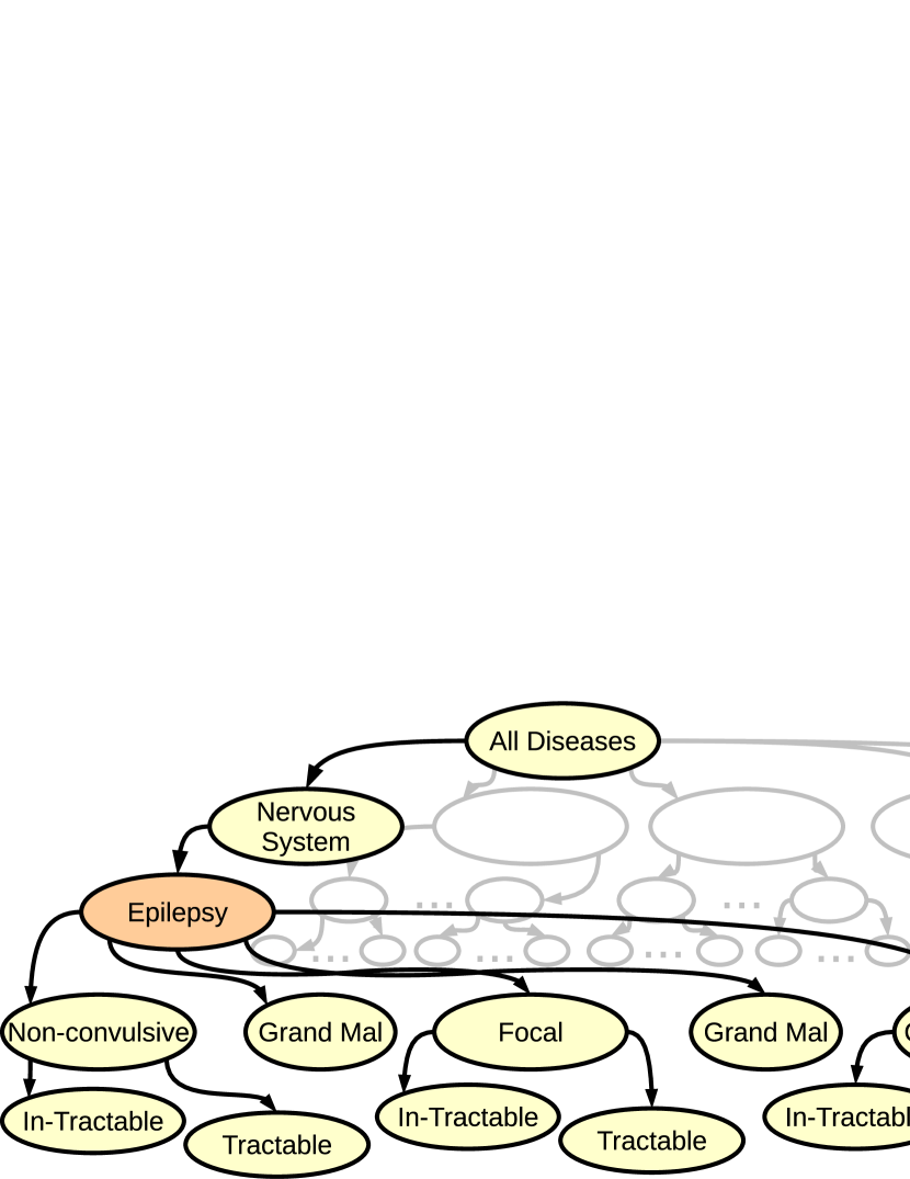
Unfortunately, existing topic modeling machinery is not equipped to capitalize on controlled structured vocabularies. We therefore propose a new model, Graph-Sparse LDA, that exploits DAG-structured vocabularies to induce interpretable topics that still summarize the data well. This approach is appropriate when documents come annotated with structured vocabulary terms, e.g., biomedical articles with MeSH headers, genes with known interactions, and species with known taxonomies. Graph-Sparse LDA introduces an additional layer of hierarchy into the standard LDA model: instead of topics being distributions over observed words, topics are distributions over concept-words, which then generate observed words using a noise process that is informed by the structure of the vocabulary (see example in figure 2). Using the structure of the vocabulary to guide the induced sparsity, we recover topics that are more interpretable to domain experts.

We demonstrate Graph-Sparse LDA on two real-world applications. The first is a collection of diagnoses for patients with autism spectrum disorder. For this we use a diagnosis hierarchy [11] to recover clinically relevant subtypes described by a small set of concepts. The second is a corpus of biomedical abstracts annotated with hierarchically-structured Medical Subject Headings (MeSH) [12]. Here, Graph-Sparse LDA identifies meaningful, concise groupings (topics) of MeSH terms for use in biomedical literature retrieval tasks. In both cases, the topic models found by Graph-Sparse LDA have the same or better predictive performance as a state-of-the-art sparse topic model (Latent IBP compound Dirichlet Allocation [8]) while providing much sparser topic descriptions. To efficiently sample from this model, we introduce a novel inference procedure that prefers moves along manifolds of constant likelihood to identify sparse solutions.

Figure 1: Simplified section of the ICD9-CM diagnostic hierarchy. Here, “Epilepsy” might be a good concept-word to summarize the very specific forms of epilepsy that are its descendants. Knowing that a patient has epilepsy may also explain instances of “Central Nervous System Disorder” or even “Disease.”

Figure 2: Example tree structure, where every node (including interior nodes) represents a vocabulary word. A concept-word can explain instances of its descendants and ancestors, e.g., if node 1 is a concept word, the matrix $P$ would only have non-zero values for the descendants and ancestors, marked in red and brown.

2 Graph-Sparse LDA

In this paper, our data are documents that are modeled using the “bag of words” representation that is common for topic models. Let the data $X$ consist of the counts of each of the $V$ words in the vocabulary for each of the $N$ documents. The standard LDA model [1] posits the following generative process for the words $w_{in}$ comprising each document (data instance) in $X$:

$$B_{n} \sim\textrm{Dirichlet}(\alpha_{B}1_{K}) A_{k} \sim\textrm{Dirichlet}(\alpha_{A}1_{V})$$ (1)

$$z_{in}\,|\,B_{n} \sim\textrm{Discrete}(B_{n}) w_{in}\,|\,z_{in},\{A_{k}\} \sim\textrm{Discrete}(A_{z_{in}})$$ (2)

where $K$ is the number of topics. The rows of the ${N\!\times\!K}$ matrix $B$ are the document-specific distributions over topics, and the ${K\!\times\!V}$ matrix $A$ represents each topic’s distribution over words. The notation $A_{k}$ refers to the $k^{th}$ row of $A$ and $B_{n}$ is the $n^{th}$ row of $B$. The $z_{in}$ encode the topic to which the $i^{th}$ word in document $n$ was assigned, and ${w_{in}\!\in 1,\ldots,V}$ is the $i^{th}$ word in document $n$. Since the words are assigned independently and identically, an ${N\times V}$ matrix of how often each word occurs in each document is a sufficient statistic for the words $w_{in}$.

Our Bayesian nonparametric model, Graph-Sparse LDA, builds upon a recent nonparametric extension of LDA, Latent IBP compound Dirichlet Allocation (LIDA) [8]. In addition to allowing an unbounded number of topics, LIDA introduces sparsity over both the document-topic matrix $B$ and the topic-word matrix $A$ using a three-parameter Indian Buffet Process. The prior expresses a preference for describing each document with few topics and each topic with few words. We extend LIDA by assuming that words in our document belong to a structured vocabulary with known relationships that form a tree or DAG, and that nearby groups of terms—as defined with respect to the graph structure—are associated with specific phenomena. For example, in a biomedical ontology, nodes on one sub-tree may correspond to a particular virus (e.g., HIV) and a different sub-tree may describe a specific drug or treatment (e.g., anti-retrovirals) used to treat HIV. Papers investigating anti-retrovirals for treatment of HIV would then tend to have terms drawn from both sub-trees. Intuitively, we would like to uncover these sub-trees as the concepts underpinning a topic.

Using concept-words to summarize the words in a topic is natural in many scenarios because structured vocabularies are often both very specific and inconsistently annotated. For example, a trial may be annotated with the term antiviral agents or its child anti-retroviral agents. Thus, from a generative modeling perspective, nearby words in the vocabulary can be thought of as having been produced from the same core concept. Our model posits that a topic is made up of a sparse set of concept-words that can explain words that are its ancestors or descendants (see Figure 2). Formally, we replace the previous LDA generative process with the following process that introduces $\tilde{w}_{in}$ as the concept word behind observed word $w_{in}$:

$$\pi_{k} \sim\textrm{IBP-Stick}(\gamma_{B}) \rho_{v} \sim\textrm{Beta}(\gamma_{A}/V,1)$$ (3)

$$\bar{B}_{n}\,|\,\pi_{k} \sim\textrm{Bernoulli}(\pi_{k}) \bar{A}_{k}\,|\,\rho_{v} \sim\textrm{Bernoulli}(\rho_{v})$$ (4)

$$B_{n}\,|\,\bar{B}_{n} \sim\textrm{Dirichlet}(\bar{B}_{n}\odot\alpha_{B}1_{K}) A_{k}\,|\,\bar{A}_{k} \sim\textrm{Dirichlet}(\bar{A}_{k}\odot\alpha_{A}1_{V})$$ (5)

$$z_{in}\,|\,B_{n} \sim\textrm{Discrete}(B_{n}) \tilde{w}_{in}\,|\,z_{in},\{A_{k}\} \sim\textrm{Discrete}(A_{z_{in}})$$ (6)

$$P_{v} \sim\textrm{Dirichlet}(\mathcal{O}_{v}\odot\alpha_{P}1_{V}) w_{in}\,|\,\tilde{w}_{in},P \sim\textrm{Discrete}(P_{\tilde{w}_{in}})$$ (7)

where $\odot$ is the element-wise Hadamard product and IBP is the Indian Buffet Process [13]. As in the standard LDA model, the document-topic matrix $B$ represents the distribution of topics in each document. However, $B_{n}$ is now masked according to a document-specific vector $\bar{B}_{n}$, which is the $n^{th}$ row of a matrix $\bar{B}$ that is itself drawn from an IBP with concentration parameter $\gamma_{B}$. Thus $\bar{B}_{nk}$ is 1 if topic $k$ has nonzero probability in document $n$ and 0 otherwise. Similarly, the topic-concept matrix $A$ and the binary topic-concept mask matrix $\bar{A}$ represent the topic matrix and its sparsity pattern, except that now $A$ and $\bar{A}$ represent the relationship between topics and concept-words. The priors over the document-topic and topic-concept matrices $B$ and $A$ (and their respective masks $\bar{B}$ and $\bar{A}$) follow those in LIDA [8].

The concept-word matrix $P$ describes distributions over words for each concept. The form of the ontology $\mathcal{O}$ determines the sparsity pattern of $P$: we use the notation $\mathcal{O}_{w}$ to refer to a binary vector of length $V$ that is 1 if the concept-word $\tilde{w}$ is a descendant or ancestor of observed word $w$ and 0 otherwise. We illustrate these sparsity constraints in Figure 2, where the dark-shaded concept nodes 1, 2, and 3 can each only explain themselves, and words that are are ancestors or descendants. The brown and green nodes are ancestor observed words that are shared by more than one concept word.

Intuitively, the concept-word matrix $P$ can be viewed as allowing for variation in the process of assigning terms to documents (citations, diagnoses, etc.) on behalf of domain experts. For example, if a document is about anti-retroviral agents, an annotator may describe the document with a key-word nearby in the vocabulary, such as antiviral agents, rather than the more specific term. Similarly, a primary care physician using the hierarchy in Figure 2 may note that a patient has epilepsy since he is not an expert in neurological disorders, while a specialist might bill for the more specific term Convulsive Epilepsy, Intractable. More generally, the concept-word matrix $P$ can be thought of as describing a neighborhood of words that could be covered by the same concept. Introducing this additional layer of hierarchy allows us to find very sparse topic-concept matrices $A$ that still explain a large number of observed words. (Note that setting ${P=I_{V}}$ recovers LIDA from Graph-Sparse LDA; Graph-Sparse LDA is therefore a generalization of LIDA that allows for much more structure.)

Finally, let the data $X$ be an ${N\times V}$ matrix of counts, where $X_{nw}$ is the number of times word $w$ appears in document $n$. The log-likelihood of the data given $B$, $A$, and $P$ is given by

$$\log p(X|A,B,P) =\sum_{n,\tilde{w}}X_{n\tilde{w}}\log(B_{n}AP_{\tilde{w}})$$ (8)

3 Inference

We describe a blocked-Gibbs procedure for sampling $B$, $\bar{B}$, $A$, $\bar{A}$, and $P$ as well as an additional Metropolis-Hastings (MH) procedure that helps the sampler to move toward sparser topic-concept word matrices $A$. Specifically, our MH proposal distribution is designed to prefer proposals of new $A^{\prime}$ and $P^{\prime}$ such that the overall likelihood does not significantly change. To our knowledge, MCMC that uses moves that result in near-constant likelihood to encourage large changes in the prior is a novel approach. We first describe how to resample instantiated parameters of the Graph-Sparse LDA model and then describe how we sample new topics.

3.1 Blocked Gibbs Sampling

Our blocked Gibbs sampling procedure relies on first sampling two intermediate assignment tensors. The first, $C_{NKV}$ counts how often the word $v$ is assigned to topic $k$ in document $n$. The second, $C_{KVV}$ counts how often each observed word is assigned to each concept word in topic $k$. These two tensors are sampled as follows:

Count Tensors $C_{NKV}$ and $C_{KVV}$:

The probability that an observed word $w$ belongs to topic $k$ is given by ${p_{nkw}=B_{nk}\sum_{\tilde{w}=1}^{V}A_{k\tilde{w}}P_{\tilde{w}w}}$ where the sum over $\tilde{w}$ marginalizes out potential concept-words. Thus we can use a multinomial distribution to allocate the counts $X_{nw}$ across the $K$ topics via ${[C_{NKV}]_{n:w}\sim\textrm{Mult}(p_{n:w},X_{nw})}$, where we use “:” to indicate a tensor slice. For updating $C_{KVV}$, the probability that $\tilde{w}$ was the generating concept word, given the observed word $w$ and the topic $k$, is given by ${p_{k\tilde{w}w}\propto A_{k\tilde{w}}P_{\tilde{w}w}}$. Thus we can sample the count tensor $C_{KVV}$ using the multinomial

$${[C_{KVV}]_{k:w}\sim\textrm{Mult}(p_{k:w},{\textstyle\sum_{n}[C_{KNV}]_{nkw}})}$$

Note that given the topic assignment for an observed word, we do not need to know from which document it came to determine the distribution over concept-word assignments. Thus, we never need to consider a four-way {document, topic, concept-word, word} count tensor during inference.

Document-Topic Assignments $B$ and $\bar{B}$:

Given the count tensor $C_{NKV}$, we can sample the sparsity mask $\bar{B}$ by marginalizing out $B$ and the $\pi_{k}$ using the formula derived in [8]. First, we note that if ${\sum_{w=1}^{V}[C_{NKV}]_{nkw}>0}$, then $\bar{B}_{nk}$ must be 1 because there exists at least one word assigned to topic $k$ in document $n$. Let $\bar{B}^{(nk=0)}$ denote the matrix $\bar{B}$, but with entry ${\bar{B}_{nk}=0}$. If ${\sum_{w=1}^{V}[C_{NKV}]_{nkw}=0}$, then the probability $\phi_{nk}$ that ${\bar{B}_{nk}=1}$ is given by

$$\psi_{nk} =\left[1+\frac{\mathcal{B}(\alpha_{B}\bar{B}^{(nk=0)}_{n},\alpha_{B})(N-\bar{B}^{(nk=0)}_{k})}{\mathcal{B}(\alpha_{B}\bar{B}^{(nk=0)}_{n}+\sum_{w=1}^{V}X_{nw},\alpha_{B})\bar{B}^{(nk=0)}_{k}}\right]^{-1}$$

where $\mathcal{B}(\cdot,\cdot)$ is the Beta function, ${\bar{B}^{(nk=0)}_{n}\equiv\sum_{k^{\prime}}\bar{B}^{(nk=0)}_{nk^{\prime}}}$, and ${\bar{B}^{(nk=0)}_{k}\equiv\sum_{n^{\prime}}\bar{B}^{(nk=0)}_{n^{\prime}k}}$. Once we have resampled $\bar{B}$, we resample $B$ using

$${B_{n}\sim\textrm{Dirichlet}(\bar{B}_{n}\odot(\alpha_{B}+{\textstyle\sum_{w=1}^{V}[C_{NKV}]_{n:w}}))}.$$

Topic-Concept Word Assignments $A$ and $\bar{A}$:

As with $\bar{B}$, we marginalize out $A$ and $\rho_{v}$ when sampling $\bar{A}$. If ${\sum_{w=1}^{V}[C_{KVV}]_{k\tilde{w}w}>0}$, then at least one observed word was assigned to topic $k$ and concept-word $\tilde{w}$, and therefore ${\bar{A}_{k\tilde{w}}=1}$. Let $\bar{A}^{(k\tilde{w}=0)}$ be the same as matrix $\bar{A}$, but with entry ${\bar{A}_{k\tilde{w}}=0}$. If ${\sum_{w=1}^{V}[C_{KVV}]_{k\tilde{w}w}=0}$, then the probability $\phi_{k\tilde{w}}$ that ${\bar{A}_{k\tilde{w}}=1}$ is given by

$$\phi_{k\tilde{w}} =\left[1+\frac{\mathcal{B}(\alpha_{A}\bar{A}^{(k\tilde{w}=0)}_{k},\alpha_{A})(K-\bar{A}^{(k\tilde{w}=0)}_{\tilde{w}}))}{(\mathcal{B}(\alpha_{A}\bar{A}^{(k\tilde{w}=0)}_{k}+\sum_{\tilde{w}}\sum_{w}[C_{KVV}]_{k\tilde{w}w},\alpha_{A})\bar{A}^{(k\tilde{w}=0)}_{\tilde{w}}}\right]^{-1}$$

where $\mathcal{B}$ is the Beta function, $K$ is the number of instantiated topics, ${\bar{A}^{(k\tilde{w}=0)}_{k}\equiv\sum_{\tilde{w}^{\prime}}\bar{A}^{(k\tilde{w}=0)}_{k\tilde{w}^{\prime}}}$, and ${\bar{A}^{(k\tilde{w}=0)}_{\tilde{w}}\equiv\sum_{k^{\prime}}\bar{A}^{(k\tilde{w}=0)}_{k^{\prime}\tilde{w}}}$. Once we have resampled $\bar{A}$, we resample $A$ via

$${A_{k}\sim\textrm{Dirichlet}(\bar{A}_{k}\odot(\alpha_{A}+{\textstyle\sum_{w}[C_{KVV}]_{k:w}}))}$$

Concept Word-Word Distributions $P$:

Finally, the concept word to observed word distributions can be resampled via

$${P_{\tilde{w}}\sim\textrm{Dirichlet}((\mathcal{O}_{\tilde{w}}>0)\odot(\alpha_{P}+{\textstyle\sum_{k}[C_{KVV}]_{k\tilde{w}:}}))}.$$

3.2 MH Moves for Improved Sparsity

Recall that one of our modeling objectives is to identify a small, interpretable set of concept-words in each topic. To this end, we have placed a sparsity-inducing prior on $A$. While the Gibbs sampling procedure above is computationally straightforward, it often does not give us the desired sparsity in $A$ fast enough. Mixing is slow because the only time we set ${\bar{A}_{k\tilde{w}}=0}$ is when no counts of $\tilde{w}$ are assigned to topic $k$ across any of the documents. When there are many documents, reaching zero counts is unlikely, and thus the sampler is slow to sparsify the topic-concept word matrix $A$.

We introduce an MH procedure to encourage moves of the topic concept-word matrix $A$ in directions of greater sparsity through joint moves on both $A$ and $P$. Given a proposal distribution $Q(A^{\prime},P^{\prime}\,|\,A,P)$, the acceptance ratio for an MH procedure is given by

$$a_{MH} =1\wedge\frac{p(X\,|\,B,A^{\prime},P^{\prime})\,p(A^{\prime})\,p(P^{\prime})\,Q(A,P\,|\,A^{\prime},P^{\prime})}{p(X\,|\,B,A,P)\,p(A)\,p(P)\,Q(A^{\prime},P^{\prime}\,|\,A,P)}$$

The sparsity-inducing prior on $A$ will prefer topic-concept word matrices $A^{\prime}$ that have more zeros. However, as with all Bayesian models (and seen in our case in Equation 8), when the data get large, the likelihood term $p(X\,|\,B,A,P)$ will dominate the prior terms $p(A)$ and $p(P)$.

To allow for moves toward greater sparsity, our MH proposal uses two core ideas. First, we use the form of the ontology to propose intelligent split-merge moves for $A^{\prime}$. Second, we attempt to make a move that keeps the likelihood as constant as possible by proposing a $P^{\prime}$ such that ${AP=A^{\prime}P^{\prime}}$. Thus, the prior terms $p(A)$ and $p(P)$ will have a larger influence on the move. The form of $Q(A^{\prime},P^{\prime}\,|\,A,P)$ is as follows:

• $Q(A^{\prime}\,|\,A,P)$: We choose a random topic $k$ and concept word $\tilde{w}$. Let $D_{\tilde{w}}$ denote the set of concept words that are descendants of $\tilde{w}$ (including $\tilde{w}$). With probability $p_{\sf{split}}$, we sample a random vector $r$ from $\textrm{Dirichlet}(1_{|D_{\tilde{w}}|})$ and create a new $A^{\prime}_{k}$ with ${A^{\prime}_{k\tilde{w}}=0}$ and ${A^{\prime}_{k\tilde{w}^{\prime}}=A_{k\tilde{w}^{\prime}}+rA_{k\tilde{w}}}$, ${\forall\tilde{w}^{\prime}\in D_{\tilde{w}}}$. Otherwise, we perform the merge ${A^{\prime}_{k\tilde{w}^{\prime}}=0}$, ${\forall\tilde{w}^{\prime}\in D_{\tilde{w}}}$, and ${A^{\prime}_{k\tilde{w}}=\sum_{\tilde{w}^{\prime}\in D_{\tilde{w}}}A_{k\tilde{w}^{\prime}}}$. This split-merge move corresponds to adjusting probabilities in a sub-graph of the ontology, with the merge move corresponding to moving all the mass to a single node.

• $Q(P^{\prime}\,|\,A^{\prime},A,P)$: Let $P^{\star}$ be the solution to the optimization problem ${\min_{\hat{P}}||AP-A^{\prime}\hat{P}||^{2}_{F}}$, where $F$ denotes the Frobenius norm, with the constraints that each row of $P^{\star}$ must lie on the simplex and respect the ontology $\mathcal{O}$. This optimization can be solved as a quadratic program with linear constraints. We then sample each row of the proposal $P^{\prime}$ according to ${P^{\prime}_{v}\sim\textrm{Dirichlet}(\beta_{MH}P^{\star}_{v})}$. We find in practice that $\beta_{MH}$ generally needs to be large in order to propose appropriately conservative moves.

While this procedure can still propose moves over the entire parameter space (thus guaranteeing Harris recurrence on the appropriate stationary distribution corresponding to the prior), it guarantees visits to sparse, high-likelihood solutions with high probability.

3.3 Adding and Deleting Topics

Finally, we describe how the number of topics in the data set is automatically learned. First, we remove any topics that are unused (that is, ${\sum_{n}\bar{B}_{nk}=0}$). To propose new topics, we first choose a random document $n$. We propose a new $A^{\prime}_{k^{\prime}}$ from the prior and propose that ${\bar{B^{\prime}}_{nk^{\prime}}=1}$. Finally, we propose a new ${B^{\prime}_{n}\sim\textrm{Dirichlet}(\alpha_{B}(\bar{B^{\prime}}_{n}\odot{\textstyle\sum_{w}[C_{NKV}]_{n:w}}))}$. The acceptance probability for adding the new topic $A_{k^{\prime}}$ is given by

$$\alpha_{\sf{add}}=1\wedge\frac{p(X_{n}\,|\,B^{\prime}_{n},A^{\prime},P)\,p(B^{\prime}_{n})\frac{\gamma_{A}}{N}}{p(X_{n}\,|\,B_{n},A,P)\,p(B_{n})}$$

where the $\frac{\gamma_{A}}{N}$ term comes from the probability of adding exactly one new topic in the IBP prior.

4 Results

We demonstrate the ability of our Graph-Sparse LDA model to find interpretable, predictive topics on one toy example and two real-world examples from biomedical domains. In each case we compare our model with the state-of-the-art Bayesian nonparametric topic modeling approach LIDA [8]. We focus on LIDA because it subsumes two other popular sparse topic models, the focused topic model [9] and sparse topic model [14], and because the proposed model is a generalization of LIDA.

All samplers were run for 250 iterations. The topic matrix product $AP$ was initialized using an LDA tensor decomposition [15] and then factored into $A$ and $P$ using an alternating minimization to find a sparse $A$ that enforced the simplex and ontology constraints. These initialization procedures reduced the burn-in time. Finally, a random 1% of each data-set was held out to compute predictive log-likelihoods.

Demonstration on a Toy Problem

We first considered a toy problem with a 31-word vocabulary arranged in a binary tree (see Figure 2). There were three underlying topics, each with only a single concept (the three darker nodes in Figure 2, labeled 1, 2, and 3). Each row in the matrix $P_{\tilde{w}}$ uniformly distributed 10% of its probability mass to the ancestors of each concept word and 90% of its probability mass to the concept word’s descendants (including itself). Each initialization of the problem had a randomly generated document-topic matrix comprising 1000 documents.

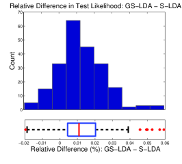
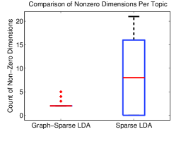
Figures 3a and 3d show the difference in the held-out test likelihoods for the final 50 samples over 20 independent instantiations of the toy problem. The difference in held-out test likelihoods is skewed positive, implying that Graph-Sparse LDA makes somewhat better predictions than LIDA. More importantly, Graph-Sparse LDA also recovers a much sparser matrix $A$, as can be seen in figure 3d. We note, of course, that Graph-Sparse LDA has an additional layer of structure that allows for a very sparse topic concept-word matrix $A$; LIDA does not have access to the ontology information $\mathcal{O}$. The important point is that by incorporating this available controlled structured vocabulary into our model, we find a solution with similar or better predictive performance than state-of-the-art models with the additional benefit of a much more interpretable structure.

(a)

(b) Autism Relative Log-LH

(c) SR Relative Log-LH

(d) Toy Topic Sparsity

(e) Autism Topic Sparsity

(f) SR Topic Sparsity

Figure 3: The top row shows the difference in held-out test log-likelihoods between Graph-Sparse LDA and Sparse LDA, divided by the overall mean held-out log-likelihood of both models after burn-in. In three domains, the predictive performance of Graph-Sparse LDA is within a few percent of LIDA. The second row shows the number of non-zero dimensions in the topic-concept word and the topic-word for Graph-Sparse LDA and LIDA models, respectively. Results are shown over 20 independent instantiations of the toy problem and 5 independent MCMC runs of the Autism and systematic review (SR) problems.

Patterns of Co-Occurring Diagnoses in Autism Spectrum Disorder

Autism Spectrum Disorder (ASD) is a complex, heterogenous disease that is often accompanied by many co-occurring conditions such as epilepsy and intellectual disability. We consider a set of 3804 patients with 3626 different diagnoses where the datum $X_{nw}$ corresponds to the number of times patient $n$ received diagnosis $w$ during the first 15 years of life. Diagnoses are organized in a tree-structured hierarchy known as ICD-9CM [11]. Diagnoses higher up in the hierarchy are less specific (such as “Diseases of the Central Nervous System” or “Epilepsy with Recurrent Seizures,” as opposed to “Epilepsy, Unspecified, without mention of intractable epilepsy”). Clinicians may encode a diagnosis at any level of the hierarchy, including less specific ones.

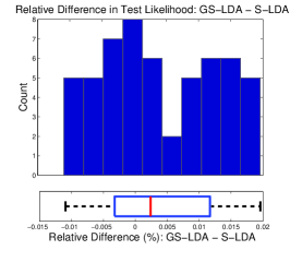
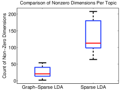
Figure 3b shows the difference in test log-likelihood between Graph-Sparse LDA and LIDA over 5 independent runs, divided by the overall mean test-likelihood value. While less pronounced than in the toy example, Graph-Sparse LDA still has slightly better predictive performance—certainly on par with current state-of-the-art topic modeling. However, the use of the ontology again allows for much sparser topics, as seen in Figure 3e. In this application, the topics correspond to possible subtypes in ASD. Being able to concisely summarize them is the first step toward using the output of this model for future clinical research.

Finally, Table 4 shows an example of one topic recovered by Graph-Sparse LDA and its corresponding topic discovered by LIDA. While the corresponding topic in LIDA has very similar diagnoses, using the hierarchy allows for Graph-Sparse LDA to summarize most of the probability mass in this topic in 6 concept words rather than 119 words. This topic—which shows a connection between the more severe form of ASD, intellectual disability, and epilepsy—as well as the other topics, matched recently published clinical results on ASD subtypes [16].

Table 1: Sample Discovered Topic using Graph-Sparse LDA on the ASD data, compared with LIDA. Graph-Sparse LDA required only 6 concepts to summarize most of probability mass in the topic, while LIDA required 119. For LIDA, we do not show all of the diagnoses associated with the topic, but only a sample of those diagnoses that are summarized by the shown concept words.

Graph-Sparse LDA	LIDA
(6 total nonzero)	(119 total nonzero)
0.333: Autistic disorder, current or active state	(1) 0.213: Autistic disorder, current or active state
0.203: Epilepsy and recurrent seizures	(15), including 0.052: Epilepsy, unspecified, without mention of intractable epilepsy, 0.0283: Localization-related epilepsy and epileptic syndromes with com, 0.023: Generalized convulsive epilepsy, without mention of intractable epilepsy, 0.008: Localization-related epilepsy and epileptic syndromes with sim, 0.006: Generalized convulsive epilepsy, with intractable epilepsy, 0.005: Epilepsy, unspecified, with intractable epilepsy, 0.004: Infantile spasms, without mention of intractable epilepsy, …
0.131: Other convulsions	(2) 0.083: Other convulsions, 0.015: Convulsions
0.055: Downs syndrome	(1) 0.001: Conditions due to anomaly of unspecified chromosome
0.046: Intellectual disability	(1) 0.034: Intellectual disability
0.040: Other Disorders of the Central Nervous System	(31), including: 0.052: Epilepsy, unspecified, without mention of intractable epilepsy, 0.006: Generalized convulsive epilepsy, with intractable epilepsy, 0.002: Other brain condition, 0.002: Quadriplegia, 0.0001: Hemiplegia, unspecified, affecting dominant side, 0.0001: Migraine without aura, with intractable migraine, 0.00009: Flaccid hemiplegia Flaccid hemiplegia and hemiparesis affecting unspecified side, 0.00005: Metabolic encephalopathy…

Medical Subject Headings for Biomedical Literature

The National Library of Medicine maintains a controlled structured vocabulary of Medical Subject Headings (MeSH) [12]. These terms are hierarchical: terms near the root are more general than those further down the tree. For example, cardiovascular diseases subsumes heart diseases, which is in turn a parent of Heart Aneurysm.

These MeSH terms are useful for searching the biomedical literature. For example, when conducting a systematic review (SR) [17], one looks to summarize the totality of the published evidence pertaining to a precise clinical question. Identifying this evidence in the literature is a time-consuming, expensive and tedious endeavor; computational methods for reducing the labor involved in this process have therefore been investigated [18, 19]. MeSH terms are helpful annotations for facilitating literature screening for systematic reviews, as they can help researchers undertaking a review quickly decide if articles are relevant to their query or not.

However, MeSH terms are manually assigned to articles by a small group of annotators. Thus, there is inherent variability in the specificity of the terms assigned to articles. This variability can make leveraging the terms difficult. Graph-Sparse LDA provides a means of identifying latent concepts that define distributions over terms nearby in the MeSH structure. These interpretable, sparse topics can provide concise summaries of biomedical documents, thus easing the evidence retrieval process for overburdened physicians.

Table 2: Sample Discovered Topic using Graph-Sparse LDA on the MeSH data for studies comprising the Calcium Channels systematic review, compared with LIDA. Superscripts denote the same term found at different locations in the MeSH structure; we collapse these when they appear sequentially in a topic. Due to space constraints we do not show all discovered topics. Graph-Sparse LDA captures the concepts “double-blind trial” and “calcium channel blockers” in one topic, which is exactly what the researchers were looking to summarize in this systematic review.

Graph-Sparse LDA	LIDA
(21 total nonzero)	(90 total nonzero)
0.565: Double-Blind Method1,2,3,4	(1) 0.353: Double-Blind Method1,2,3,4
0.110: Calcium Channel Blockers1,2	(7) 0.031 Adrenergic beta-Antagonists1, 0.026 Drug Therapy, Combination, 0.022 Calcium Channel Blockers, 0.016 Felodipine, 0.015 Atenololm, 0.006 Benzazepines, 0.01 Mibefradil1,2
0.095: Angina Pectoris1,2	(3) 0.030: Angina Pectoris2, 0.030: Myocardial Ischemia1,2, 0.003: Atrial Flutter

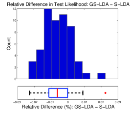
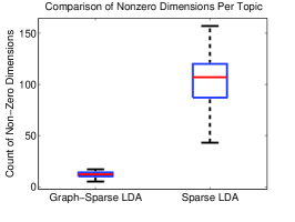
We consider a dataset of 1218 documents annotated with 5347 unique MeSH terms (23 average terms per document) that were screened for a systematic review of the effects of calcium-channel blocker (CCB) drugs [18]. In figure 3c, we see that the test log-likelihood for Graph-Sparse LDA on these data is on par with LIDA, while producing a much sparser summary of concept-words (figure 3f). Here, the concepts found by Graph-Sparse LDA correspond to sets of MeSH terms that might help researchers rapidly identify studies reporting results for trials investigating the use of CCB’s—without having to make sense of a topic comprising hundreds of unique MeSH terms.

Table 2 shows the top concept-words in a sample topic discovered by Graph-Sparse LDA compared to a similar topic discovered by LIDA. Graph-Sparse LDA gives most of topic mass to double-blind trials and CCBs; knowing the relative prevalence in an article of this topic would clearly help a researcher looking to find reports of randomized controlled trials of CCBs. In contrast, words related to concept CCBs are divided among terms in LIDA. Some of the LIDA terms, such as Drug Therapy, Combination and Mibefradil are also present in Graph-Sparse LDA, but with much lower probability – the concept CCB summarizes most of the instances. We note that a professional systematic reviewer at [Anonymous] confirmed that the more concise topics found by Graph-Sparse LDA would be more useful in facilitating evidence retrieval tasks than those found by LIDA.

5 Discussion and Related Work

Topic models [1, 2] have gained wide popularity as a flexible framework for uncovering latent structure in corpora. Existing topic models have typically assumed that observed words are unstructured. By contrast, here we have considered scenarios in which these words are drawn from a known underlying structure (such as an ontology).

Prior work in interpretable topic models has focused on various notions of coherence. [20] introduced the idea of “intrusion detection” where they hypothesized that a more coherent, or interpretable, topic would be one where a human annotator would be able to identify an inserted “intruder” word among the top 5 words in a topic; [21] automated this process. Contrary to expecation, they found that interpretability (as rated by human annotators) was negatively correlated with test likelihood. [22] and [23] developed measures of topic coherence that strongly correlated with human annotations of topic quality.

However, the evaluations in all of these works still focus only on the top $n$ words in a topic (which powerfully indicates how linked sparsity is to interpretability; humans have trouble working with long lists). In contrast, our approach does not sacrifice on predictive quality and, by using the ontological structure, provides a compact summary that describes most of the words, not just the top $n$. This quality is particularly valuable in the kinds of scenarios that we described, where annotation disagreement or diagnostic “slosh” can result in a large number of words with non-trivial probabilities.

This use of a human-provided structure to induce interpretability also distinguishes Graph-Sparse LDA from other hierarchical and tree structured topic models where the structure is typically learned. For example, [24] use a nested Chinese Restaurant Process to learn hierarchies of topics where subtopics are more specific than their parents. [25] expand on this idea with a nonparametric Markov model that allows a subtopic to have multiple parents. [26] develop inference techniques for sparse versions of these tree-structured topic models. Learned hierarchies have also been used to capture correlations between topics, such as [27]. In all of these models, the learned hiearchical structure allows for various kinds of statistical sharing between the topics. However, each topic is still a distribution over a large vocabulary, and the interpretation task is only complicated by requiring a human to now both inspect the hierarchy and the topics for structure.

Among the fully unsupervised approaches, the closest to our work is the super-word concept modeling of [28], which uses a nested Beta process to describe a document with a sparse set of super-words, or concepts, each of which are associated with a sparse set of words. Known auxiliary information about the words, encoded in a feature vector, can be used to encourage or discourage words from being part of the same concept. A key difference in our approach is that we use the graph structure to guide the formation of concepts, which maintains interpretability while removing the need for each concept to have a sparse set of words. Our graph-structured relationships also result in a much simpler inference procedure.

While not applied to increase interpretability, expert-defined hierarchies have been used in topic models in other contexts. Early work by [29] used hierarchies for word-sense disambiguation in n-gram tuples. This idea was later incorporated into a topic modeling context by [30]. Other work has used hierarchical structure as partial supervision to improve topic-modeling output in scenarios in which some words come from controlled vocabularies (or have known relationships) and others do not. [31] consider representing the content of website summaries via a hierarchical model. Their approach exploits ontological structure by jointly modeling word and ontology term generation. They showed that their model (which leverages the hierarchical document labels) improved on existing approaches with respect to perplexity. [32] use Dirichlet forest priors to enforce expert-provided “must be in same topic” and “cannot be in same topic” constraints between words. Finally, [33] propose a hierarchically supervised LDA model where there is a hierarchy on the document labels (rather than on the vocabulary). Specifically, they treat categories as ‘labels’ and model the assignment of these to documents via (probit) regression models. Their model stipulates that when a node is assigned to a category so too are all of its parents, thus capturing the hierarchical structure. In contrast to all of these works, which focus on prediction tasks, Graph-Sparse LDA uses the ontology in a probabilistic — rather than enforced — manner to obtain sparse topics from extant controlled vocabularies.

We note that our word generation model is much more general than other approaches. Here we have considered scenarios in which the ontological structure allows a concept-word to generate words that are its descendants and ancestors. However, we can imagine that a concept-word can generate any nearby observed word, where the definition of “nearby” is entirely up to the model-designer (concretely, “nearby” corresponds to the sparsity pattern in the matrix $P$). This difference allows for much more flexibility in modeling: the underlying structure can be a tree, a DAG, or just some collection of neighborhoods. At the same time, our formulation results in a Gibbs sampling procedure that is simpler than many other hierarchical models.

6 Conclusions

Topic models have revolutionized prediction and classification models in many domains, and many scientists are now attempting to use them to uncover structure from their data. For these applications, however, prediction is not enough: scientists wish to be able to understand the structure in order to posit new theories. At the same time, structured knowledge-bases often exist for scientific domains; these are information dense resources that capture a wealth of expertise.

In this paper we have proposed a model that exploits such resources to achieve the stated aim of identifying interpretable topics. More specifically, we have described a novel Bayesian nonparametric model, Graph-Sparse LDA, that leverages existing controlled vocabulary structures to induce interpretable topics. The Bayesian nonparametric aspect of the model allows us to discover the number of topics in our dataset. Leveraging ontological knowledge allows us to uncover sparse sets of concept words that provide succinct, interpretable topic summaries that maintain the ability to explain a large number of observed words. The combination of this representational power and an efficient inference procedure allowed us to realize topic interpretability while still matching (and often exceeding) state-of-the-art predictive performance.

While we have focused on controlled vocabularies in the biomedical domain, this approach could be more generally applied to text corpora using standard hierarchies such as WordNet [34]. In these more general domains, using hierarchies could eliminate the need for basic pre-processing such as stemming. This model is relatively straight-forward to implement, and we expect it to be useful for a variety of topic or factor-discovery applications where the observed dimensions have some human-understandable relationships.

Acknowledgments

We are grateful to Isaac Kohane and the i2b2 team at Boston Children’s Hospital for providing us the autism data and their feedback on the GS-LDA model as a data-mining tool.

References

- [1] D. M. Blei, A. Y. Ng, and M. I. Jordan, “Latent Dirichlet allocation,” Journal of Machine Learning Research, vol. 3, pp. 993–1022, 2003.
- [2] M. Steyvers and T. Griffiths, “Probabilistic topic models,” Handbook of latent semantic analysis, vol. 427, no. 7, pp. 424–440, 2007.
- [3] D. M. Blei, “Probabilistic topic models,” Communications of the ACM, vol. 55, no. 4, pp. 77–84, 2012.
- [4] T. L. Griffiths and M. Steyvers, “Finding scientific topics,” Proceedings of the National Academy of Sciences of the United States of America, vol. 101, pp. 5228–5235, 2004.
- [5] L. Fei-Fei and P. Perona, “A Bayesian hierarchical model for learning natural scene categories,” in CVPR, vol. 2, pp. 524–531, 2005.
- [6] Y. Wang and G. Mori, “Human action recognition by semilatent topic models,” IEEE Transactions on Pattern Analysis and Machine Intelligence, vol. 31, no. 10, pp. 1762–1774, 2009.
- [7] M. Ghassemi, T. Naumann, R. Joshi, and A. Rumshisky, “Topic models for mortality modeling in intensive care units,” in ICML 2012 Machine Learning for Clinical Data Analysis Workshop, 2012.
- [8] C. Archambeau, B. Lakshminarayanan, and G. Bouchard, “Latent IBP compound Dirichlet allocation,” in NIPS Bayesian Nonparametrics Workshop, 2011.
- [9] S. Williamson, C. Wang, K. A. Heller, and D. M. Blei, “The IBP compound Dirichlet process and its application to focused topic modeling,” in ICML, pp. 1151–1158, 2010.
- [10] J. Eisenstein, A. Ahmed, and E. P. Xing, “Sparse additive generative models of text,” in ICML, 2011.
- [11] O. Bodenreider, “The unified medical language system (UMLS): integrating biomedical terminology,” Nucleic acids research, vol. 32, pp. D267–D270, 2004.
- [12] C. E. Lipscomb, “Medical subject headings (MeSH),” Bull Med Libr Assoc., 2000. 88(3): 265–266.
- [13] T. Griffiths and Z. Ghahramani, “The Indian buffet process: An introduction and review.,” Journal of Machine Learning Research, vol. 12, pp. 1185–1224, 2011.
- [14] C. Wang and D. Blei, “Decoupling Sparsity and Smoothness in the Discrete Hierarchical Dirichlet Process,” in Advances in Neural Information Processing Systems 22 (Y. Bengio, D. Schuurmans, J. Lafferty, C. K. I. Williams, and A. Culotta, eds.), pp. 1982–1989, 2009.
- [15] A. Anandkumar, R. Ge, D. Hsu, S. M. Kakade, and M. Telgarsky, “Tensor decompositions for learning latent variable models.” http://arxiv.org/abs/1210.7559, 2012.
- [16] F. Doshi-Velez, Y. Ge, and I. Kohane, “Comorbidity clusters in autism spectrum disorders: An electronic health record time-series analysis.,” Pediatrics, 2013.
- [17] J. M. Grimshaw and I. T. Russell, “Effect of clinical guidelines on medical practice: a systematic review of rigorous evaluations,” The Lancet, vol. 342, no. 8883, pp. 1317–1322, 1993.
- [18] A. M. Cohen, W. R. Hersh, K. Peterson, and P.-Y. Yen, “Reducing workload in systematic review preparation using automated citation classification,” Journal of the American Medical Informatics Association, vol. 13, no. 2, pp. 206–219, 2006.
- [19] B. C. Wallace, K. Small, C. E. Brodley, and T. A. Trikalinos, “Active learning for biomedical citation screening,” in KDD, pp. 173–182, 2010.
- [20] J. Chang, J. L. Boyd-Graber, S. Gerrish, C. Wang, and D. M. Blei, “Reading tea leaves: How humans interpret topic models,” in NIPS, pp. 288–296, 2009.
- [21] J. H. Lau, D. Newman, and T. Baldwin, “Machine reading tea leaves: Automatically evaluating topic coherence and topic model quality,” in 14th Conference of the European Chapter of the Association for Computational Linguistics (EACL), 2014.
- [22] D. Newman, J. H. Lau, K. Grieser, and T. Baldwin, “Automatic evaluation of topic coherence,” in Human Language Technologies: The 2010 Annual Conference of the North American Chapter of the Association for Computational Linguistics, HLT ’10, pp. 100–108, Association for Computational Linguistics, 2010.
- [23] D. Mimno, H. Wallach, E. Talley, M. Leenders, and A. McCallum, “Optimizing semantic coherence in topic models,” in EMNLP, 2011.
- [24] D. M. Blei, T. L. Griffiths, and M. I. Jordan, “The nested Chinese restaurant process and Bayesian nonparametric inference of topic hierarchies,” Journal of the ACM, vol. 57, no. 2, pp. 7:1–7:30, 2010.
- [25] H. Chen, D. B. Dunson, and L. Carin, “Topic modeling with nonparametric Markov tree,” in ICML, pp. 377–384, 2011.
- [26] Y. Hu and J. Boyd-Graber, “Efficient tree-based topic modeling,” in ACL, 2012.
- [27] W. Li and A. McCallum, “Pachinko allocation: DAG-structured mixture models of topic correlations,” in ICML, pp. 577–584, 2006.
- [28] K. El-Arini, E. B. Fox, and C. Guestrin, “Concept modeling with superwords.” http://arxiv.org/abs/1204.2523, 2012.
- [29] S. Abney and M. Light, “Hiding a semantic hierarchy in a Markov model,” in Workshop on Unsupervised Learning in Natural Language Processing, pp. 1–8, 1999.
- [30] J. L. Boyd-Graber, D. M. Blei, and X. Zhu, “A topic model for word sense disambiguation,” in EMNLP-CoNLL, pp. 1024–1033, 2007.
- [31] A. Slutsky, X. Hu, and Y. An, “Tree labeled LDA: A hierarchical model for web summaries,” in IEEE International Conference on Big Data, pp. 134–140, 2013.
- [32] D. Andrzejewski, X. Zhu, and M. Craven, “Incorporating domain knowledge into topic modeling via Dirichlet forest priors,” in ICML, pp. 25–32, 2009.
- [33] A. J. Perotte, F. Wood, N. Elhadad, and N. Bartlett, “Hierarchically supervised latent Dirichlet allocation,” in NIPS, pp. 2609–2617, 2011.
- [34] G. A. Miller, “Wordnet: A lexical database for English,” Communications of the ACM, vol. 38, pp. 39–41, 1995.