Fast detection of cycles in timed automata

Abstract

We propose a new efficient algorithm for detecting if a cycle in a timed automaton can be iterated infinitely often. Existing methods for this problem have a complexity which is exponential in the number of clocks. Our method is polynomial: it essentially does a logarithmic number of zone canonicalizations. This method can be incorporated in algorithms for verifying Büchi properties on timed automata. We report on some experiments that show a significant reduction in search space when our iteratability test is used.

1 Introduction

Timed automata [1] are one of the standard models of timed systems. There has been an extensive body of work on the verification of safety properties on timed automata. In contrast, advances on verification of liveness properties are much less spectacular due to fundamental challenges that need to be addressed. For verification of liveness properties, expressed in a logic like Linear Temporal Logic, it is best to consider a slightly more general problem of verification of Büchi properties. This means verifying if in a given timed automaton there is an infinite path passing through an accepting state infinitely often.

Testing Büchi properties of timed systems can be surprisingly useful. We give an example in Section 5 where we describe how with a simple liveness test one can discover a typo in the benchmark CSMA-CD model. This typo removes practically all interesting behaviours from the model. Yet the CSMA-CD benchmark has been extensively used for evaluating verification tools, and nothing unusual has been observed. Therefore, even if one is interested solely in verification of safety properties, it is important to “test” the model under consideration, and for this Büchi properties are indispensable.

Verification of timed automata is possible thanks to zones and their abstractions [12, 3, 19]. Roughly, the standard approach used nowadays for verification of safety properties performs breadth first search (BFS) over the set of pairs (state, zone) reachable in the automaton, storing only pairs with the maximal abstracted zones (with respect to inclusion).

The fundamental problem in extending this approach to verification of Büchi properties is that it is no longer sound to keep only maximal zones with respect to inclusion. Laarman et al. [21] recently studied in depth when it is sound to use zone inclusion in nested depth first search (DFS). The inability to make use of zone inclusions freely has a very important impact on the search space: it can simply get orders of magnitude larger, and this indeed happens on standard examples.

The second problem with verification of Büchi properties is that fact that we need to use DFS instead of BFS to detect cycles. It has been noted in numerous contexts that longer sequences of transitions lead generally to smaller zones [2]. This is why BFS would often find the largest zones first, while DFS will get very deep into the model and consider many small zones; these in turn will be made irrelevant later with a discovery of a bigger zone closer to the root. Once again, on standard examples, the differences in the size of the search space between BFS and DFS exploration are often significant [2], and it is rare to find instances where DFS is better than BFS.

In this paper we propose an efficient test for checking $\omega$-iterability of a path in a timed automaton. By this we mean checking if a given sequence of timed transitions can be iterated infinitely often. We then use this test to ease the bottleneck created by the two above mentioned problems. While we will still use DFS, we will invoke $\omega$-iterability test to stop exploration as early as possible. In the result, we will not gain anything if there is no accepting loop, but if there is one we will often discover it much quicker.

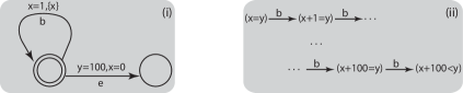
Figure 1: Iterability of $b$ transtion in timed automaton (i) requires a long exloration in the zone graph (ii).

An example of $\omega$-iterability checking is presented in Figure 1. The zone graph of the automaton has $100$ states due to the difference between $y$ and $x$ that gets bigger after each iteration of $b$ transition. As the maximum constant for $y$ is $100$, the zones obtained after $x+100=y$ will get abstracted to $x+100<y$, giving a cycle on the zone graph. Without iterability testing we need to take all these transitions to conclude that $b$ can be iterated infinitely often. In contrast, our iterability test applied to $b$ transition can tell us this immediately.

A simple way to decide if a sequence of timed transitions $\sigma$ is iterable is to keep computing successive regions along $\sigma$ till a region repeats. However one might have to iterate $\sigma$ as many times as the number of regions. Hence the bound on the number of iterations given by this approach is $\mathcal{O}(|\sigma|\cdot M!\cdot 2^{n})$ where $n$ is the number of clocks and $M$ is the maximum constant occurring in the automaton. Using zones instead of regions does not change much: we still may need to iterate $\sigma$ an exponential number of times in $n$.

Our solution uses transformation matrices which are zone like representations of the effect of a sequence of timed transitions. Such matrices have already been used by Comon and Jurski in their work on flattening of timed automata [9]. By analysing properties of these matrices we show that $n^{2}$ iterations of $\sigma$ are sufficient to determine $\omega$-iterability. Moreover, instead of doing these iterations one can simply do $\log(n^{2})$ compositions of transformation matrices. As a bonus we obtain a zone describing all the valuations from which the given sequence of transitions is $\omega$-iteratable. The complexity of the procedure is $\mathcal{O}((|\sigma|+\log n)\cdot n^{3})$.

One should bear in mind that $n$ is usually quite small, as it refers only to active clocks in the sequence. Recall for example that zone canonisation, that is $\mathcal{O}(n^{3})$ algorithm, is anyway evoked at each step of the exploration algorithm. If we assume that arithmetic operations can be done in unit time, the complexity of our algorithm does not depend on $M$.

One should bear in mind that $n$ is usually quite small, as it refers only to active clocks in the sequence. Recall for example that zone canonicalisation, that is an $\mathcal{O}(n^{3})$ algorithm, is anyway evoked at each step of the exploration algorithm. If we assume that arithmetic operations can be done in unit time, the complexity of our algorithm does not depend on $M$.

Apart from the theoretical gains of the $\omega$-iteratability test mentioned above, we have also observed substantial gains on standard benchmarks. We have done a detailed examination of standard timed models as used, among others, in [21]. We explain in Section 5 why when checking for false Büchi properties that do not refer to time on these models, the authors of op. cit. have observed almost immediate response. Our experiments show that even on these particular models, if we consider a property that refers to time, the situation changes completely. We present examples of timed Büchi properties where iteration check significantly reduces the search space.

Related work

Acceleration of cycles in timed automata is technically the closest work to ours. The binary reachability relation of a timed automaton can be expressed in Presburger arithmetic by combining cycle acceleration [8, 6, 4] and flattening of timed automata [9]. Concentrating on $\omega$-iterability allows to assume that all clock variables are reset on the path. This has important consequences as variables that are not reset can act as counters ranging from $0$ to the maximal constant $M$ appearing in the guards. Indeed, since checking emptiness of flat automata is in Ptime, general purpose acceleration techniques need to introduce a blowup. By concentrating on a less general problem of $\omega$-iterability, we are able to find simpler and more efficient algorithm.

The $\omega$-iterability question is related to proving termination of programs. A closely related paper is [5] where the authors study conditional termination problem for a transition given by a difference bound relation. The semantics of the relation is different though as it is considered to be over integers and not over positive reals as we do here. So, for example, a cycle that strictly decreases the difference between two clocks is iterable in our sense but not in [5]. More precisely, Lemma 1 of this paper is not true over integers. The decision procedure in op. cit. uses policy iteration algorithm, and is exponential in the size of the matrix.

Tiwari [23] shows decidability of termination of simple loops in programs where variables range over reals and where the body is a set of linear assignments. This setting is different from ours since programs are deterministic and hence every state has a unique trajectory. Proving termination and nontermination for a much more general class of programs is addressed in [10, 15]

The already mentioned work of Laarman et al. [21] examines in depth the problem of verification of Büchi properties of timed systems. It focuses on parallel implementation of a modification of the nested DFS algorithm. In Section 5 we report on the experiments of using $\omega$-iterability checking in the (single processor) implementation of this algorithm.

Organization of the paper

Section 2 starts with required preliminaries. Section 3 studies $\omega$-iteratability, and describes the transformation graphs that we use to detect $\omega$-iterability. Certain patterns in these graphs would help us conclude iteratability as shown in Section 4. Finally, Section 5 gives some experimental results.

2 Preliminaries

We adopt standard definition of timed automaton without diagonal constraints. Below we state formally the Büchi non-emptiness problem, and outline how it is solved using zones and abstractions of zones. All the material in this section is well-known.

Let $\mathbb{R}_{\geq 0}$ denote the set of non-negative reals. A clock is a variable that ranges over $\mathbb{R}_{\geq 0}$. Let $X=\{x_{0},x_{1},\dots,x_{n}\}$ be a set of clocks. The clock $x_{0}$ will be special and will represent the reference point to other clocks. A valuation is a function $v\,:\,X\rightarrow\mathbb{R}_{\geq 0}$ that is required to map $x_{0}$ to $0$. The set of all clock valuations is denoted by $\mathbb{R}_{\geq 0}^{X}$. We denote by $\mathbf{0}$ the valuation that associates $0$ to every clock in $X$.

A clock constraint $\phi$ is a conjunction of constraints of the form $x\sim c$ where $x\in X\setminus\{x_{0}\}$, $\sim\in\{<,\leq,=,\geq,>\}$ and $c\in\mathbb{N}$. For example, $(x_{1}\leq 3\wedge x_{2}>0)$ is a clock constraint. Let $\Phi(X)$ denote the set of clock constraints over the set of clocks $X$. We write $v\vDash\phi$ when the valuation satisfies the constraint. We denote by $v+\delta$ the valuation where $\delta$ is added to every clock; and by $[R]v$ we denote the valuation where all clocks from $R$ are set to $0$.

A Timed Büchi Automaton (TBA in short) [1] is a tuple $\mathcal{A}=(Q,q_{0},X,T,F)$ in which $Q$ is a finite set of states, $q_{0}$ is the initial state, $X$ is a finite set of clocks, $F\subseteq Q$ is a set of accepting states, and $T\,\subseteq\,Q\times\Phi(X)\times 2^{X}\times Q$ is a finite set of transitions of the form $(q,g,R,q^{\prime})$ where $g$ is a clock constraint called the guard, and $R$ is a set of clocks that are reset on the transition from $q$ to $q^{\prime}$.

The semantics of a TBA $\mathcal{A}=(Q,q_{0},X,T,F)$ is given by a transition system of its configurations. A configuration of $\mathcal{A}$ is a pair $(q,v)\in Q\times\mathbb{R}_{\geq 0}^{X}$, with $(q_{0},\mathbf{0})$ being the initial configuration. The transitions here are of the form: $(q,v)\xrightarrow{t}^{\raisebox{-3.01389pt}{\scriptsize$\delta$}}(q^{\prime},v^{\prime})$ for some transition $t=(q,g,R,q^{\prime})\in T$ such that $(v+\delta)\vDash g$ and $v^{\prime}=[R](v+\delta)$.

A run of $\mathcal{A}$ is a (finite or infinite) sequence of transitions starting from the initial configuration $(q_{0},\mathbf{0})$. A configuration $(q,v)$ is said to be accepting if $q\in F$. An infinite run satisfies the Büchi condition if it visits accepting configurations infinitely often. The run is Zeno if time does not diverge, that is, $\sum_{i\geq 0}\delta_{i}\leq c$ for some $c\in\mathbb{R}_{\geq 0}$. Otherwise it is non-Zeno. The problem we are interested is termed the Büchi non-emptiness problem.

Definition 1

The Büchi non-emptiness problem for TBA is to decide if $\mathcal{A}$ has a non-Zeno run satisfying the Büchi condition.

The Büchi non-emptiness problem is known to be Pspace-complete [1]. All solutions to this problem construct an untimed Büchi automaton with an equivalent non-emptiness problem. We describe such a translation below.

The standard algorithms on timed automata consider special sets of valuations called zones. A zone is a set of valuations described by a conjunction of two kinds of constraints: either $x_{i}\sim c$ or $x_{i}-x_{j}\sim c$ where $x_{i},x_{j}\in X$, $c\in\mathbb{Z}$ and $\sim\in\{<,\leq,=,>,\geq\}$. For example $x_{1}>3$ and $x_{2}-x_{1}\leq-4$ is a zone. Zones can be efficiently represented by Difference Bound Matrices (DBMs) [13].

The zone graph $ZG(\mathcal{A})$ of a TBA $\mathcal{A}$ is a Büchi automaton $(S,s_{0},\Rightarrow,F)$, where $S$ is the set of states, $s_{0}$ is the initial state and $\Rightarrow$ is the transition relation. Each state in $S$ is a pair $(q,Z)$ consisting of a state $q$ of the TBA and a zone $Z$. The initial node $s_{0}$ is $(q_{0},Z_{0})$ where $Z_{0}=\{\mathbf{0}+\delta~{}|~{}\delta\in\mathbb{R}_{\geq 0}\}$. For every $t=(q,g,R,q^{\prime})\in T$, there exists a transition $\Rightarrow^{t}$ from a node $(q,Z)$ as follows:

$$(q,Z)\Rightarrow^{t}(q^{\prime},Z^{\prime})\qquad\text{where }Z^{\prime}=\{v^{\prime}~{}|~{}\exists v\in Z,~{}\exists\delta\in\mathbb{R}_{\geq 0}:(q,v)\xrightarrow{t}^{\delta}(q^{\prime},v^{\prime})\}$$

The transition relation $\Rightarrow$ is the union of $\Rightarrow^{t}$ over all $t\in T$. It can be shown that if $Z$ is a zone, then $Z^{\prime}$ is a zone. Although the zone graph $ZG(\mathcal{A})$ deals with sets of valuations instead of valuations themselves, the number of zones is still infinite [12].

For effectiveness, zones are further abstracted. An abstraction operator is a function $\mathfrak{a}:\mathcal{P}(\mathbb{R}_{\geq 0}^{|X|})\to\mathcal{P}(\mathbb{R}_{\geq 0}^{|X|})$ such that $W\subseteq\mathfrak{a}(W)$ and $\mathfrak{a}(\mathfrak{a}(W))=\mathfrak{a}(W)$ for every set of valuations $W\in\mathcal{P}(\mathbb{R}_{\geq 0}^{|X|})$. If $\mathfrak{a}$ has a finite range then this abstraction is said to be finite. An abstraction operator defines an abstract symbolic semantics:

$$(q,Z)\Rightarrow^{t}_{\mathfrak{a}}(q^{\prime},\mathfrak{a}(Z^{\prime}))\qquad\text{ when $\mathfrak{a}(Z)=Z$ and $(q,Z)\Rightarrow^{t}(q^{\prime},Z^{\prime})$ in $ZG(\mathcal{A})$}$$

We define a transition relation $\Rightarrow_{\mathfrak{a}}$ to be the union of $\Rightarrow^{t}_{\mathfrak{a}}$ over all transitions $t$. Given a finite abstraction operator $\mathfrak{a}$, the abstract zone graph $ZG^{\mathfrak{a}}(\mathcal{A})$ is a Büchi automaton whose nodes consist of pairs $(q,Z)$ such that $Z=\mathfrak{a}(Z)$. The initial state is given by $(q_{0},\mathfrak{a}(Z_{0}))$ where $(q_{0},Z_{0})$ is the initial state of $ZG(\mathcal{A})$. Transitions are given by the $\Rightarrow_{\mathfrak{a}}$ relation. The accepting states are nodes $(q,Z)$ with $q\in F$.

The abstraction operator $\mathsf{Extra}_{LU}^{+}$ [3] is a commonly used efficient abstraction operator. For concreteness we will adopt this operator in the paper, but our approach can be also used with other abstraction operators as for example $a_{LU}$ [18]. Thus we will consider the Buchi automaton given by $ZG^{\mathsf{Extra}_{LU}^{+}}(\mathcal{A})$, which is the abstract zone graph of $\mathcal{A}$ with respect to $\mathsf{Extra}_{LU}^{+}$. The following fact guarantees soundness of this approach.

Theorem 2.1 ([22])

A timed Büchi automaton $\mathcal{A}$ has a Büchi run iff the finite Büchi automaton $ZG^{\mathsf{Extra}_{LU}^{+}}(\mathcal{A})$ has one.

Theorem 2.1 gives an algorithm for non-emptiness of TBA: given a timed Büchi automaton $\mathcal{A}$, it computes the (finite) Büchi automaton $ZG^{\mathsf{Extra}_{LU}^{+}}(\mathcal{A})$ and checks for its emptiness. The main problem with this approach is efficiency. When checking for reachability it enough to consider only maximal zones with respect to inclusion of $ZG^{\mathsf{Extra}_{LU}^{+}}(\mathcal{A})$. This optimization gives very important perfomance gains, but unfortunately it is not sound for verification of Büchi properties [21]. The above theorem does not address the non-Zenoness issue. Since this issue does not influence our $\omega$ iterability test, we defer it to the conclusions.

3 $\omega$-iterability

Since we cannot use zone inclusion to cut down the search space, it can very well happen that an exploration algorithm comes over a path that can be iterated infinitely often but it is not able to detect it since the initial and final zones on the path are different. In this section we show how to test, in a relatively efficient way, if a sequence of timed transitions can be iterated infinitely often (Theorem 4.1).

Consider a sequence of transitions $\sigma$ of the form $\xrightarrow{t_{1}}\dots\xrightarrow{t_{k}}$, and suppose that $(q,Z)\Rightarrow^{\sigma}(q,Z^{\prime})$. If $Z\subseteq Z^{\prime}$ then after executing $\sigma$ from $(q,Z^{\prime})$ we obtain $(q,Z^{\prime\prime})$ with $Z^{\prime\prime}$ not smaller than $Z^{\prime}$. So we can execute $\sigma$ one more time etc. The challenging case is when $Z\not\subseteq Z^{\prime}$. The procedure we propose will not only give a yes/no answer but will actually compute the zone representation of the set of valuations from which the sequence can be iterated infinitely often. We will start by making the notion of $\omega$-iterability precise.

An execution of a sequence $\sigma$ of the form $\xrightarrow{t_{1}}\dots\xrightarrow{t_{k}}$ is a sequence of valuations $v_{0},\dots,v_{k}$ such that for some $\delta_{1},\dots\delta_{k}\in\mathbb{R}^{+}$ we have

$$v_{0}\xrightarrow{t_{1}}^{\delta_{1}}v_{1}\xrightarrow{t_{2}}^{\delta_{2}}\dots\xrightarrow{t_{k}}^{\delta_{k}}v_{k}$$

In this case we write $v_{0}\xrightarrow{\sigma}^{\delta}v_{k}$ where $\delta=\delta_{1}+\dots+\delta_{k}$. The sequence $\sigma$ is executable from $v$ if there is a sequence of valuations $v_{0},\dots,v_{k}$ as above with $v=v_{0}$. (For clarity of presentation, we choose not to write the state component of configurations $(q,v)$ and instead write $v$ alone.)

Definition 2

The sequence $\sigma$ is $\omega$-iterable if there is an infinite sequence of valuations $v=v_{0},v_{1},\dots$ and an infinite sequence of delays $\delta_{1},\delta_{2},\dots$ such that

$$v_{0}\xrightarrow{\sigma}^{\delta_{1}}v_{1}\xrightarrow{\sigma}^{\delta_{2}}\dots$$

We also say that the sequence $\sigma$ is $\omega$-iterable from $v_{0}$.

Using region abstraction one can observe the following characterization of $\omega$-iteratability in terms of finite executions. Observe that the lemma talks about $\omega$-iterability not about iterability from a particular valuation (that would give a weaker statement).

Lemma 1

A sequence of transitions is $\omega$-iterable iff for every $n=1,2,\dots$ the $n$-fold concatenation of $\sigma$ has an execution.

Proof.

Suppose a sequence of transitions $\sigma$ is $\omega$-iterable. Then, clearly every $n$-fold concatenation has an execution.

Suppose every $n$ fold concatenation of $\sigma$ has an execution. Let $r$ be the number of regions with respect to the biggest constant appearing in the automaton. By assumption, the $r$-fold concatenation of $\sigma$ has an execution:

$$v_{0}\xrightarrow{\sigma}^{\delta_{1}}v_{1}\xrightarrow{\sigma}^{\delta_{2}}v_{2}\dots v_{r-1}\xrightarrow{\sigma}^{\delta_{r-1}}v_{r}$$

In the above execution, there exist $i,j$ such that $v_{i}$ and $v_{j}$ belong to the same region $R$, thus giving a cycle in the region graph of the form $R\xrightarrow{(j-i)\sigma}R$. By standard properties of regions, $\sigma$ is $\omega$-iterable from every valuation in $R$.∎∎

The above proof shows that $\sigma$ is $\omega$-iterable iff it is $(r+1)$-iterable, where $r$ is the number of regions. As $r$ is usually very big, testing $(r+1)$-iterablity directly is not a feasible solution. Later we will show a much better bound than $(r+1)$, and also propose a method to avoid checking $k$-iterability by directly executing all the $\sigma^{k}$ transitions.

Our iterability test will first consider some simple cases when the answer is immediate using which it will remove clocks that are not relevant. This preprocessing step is explained in the following two facts. We use $X$ for the set of clocks appearing on a sequence of transitions $\sigma$, and $X_{0}$ for the set of clocks that are reset on $\sigma$. Let $\preccurlyeq$ denote either $<$ or $\leq$, and let $\succcurlyeq$ stand for $>$ or $\geq$.

Lemma 2

A sequence of transitions $\sigma$ is not $\omega$-iterable if it satisfies one of the following conditions:

• for some clock $y\in X\setminus X_{0}$, we have guards $y\preccurlyeq d$ and $y\succcurlyeq c$ in $\sigma$ such that either $d<c$, or $(d=c\text{ and }\preccurlyeq=<)$, or $(d=c\text{ and }\succcurlyeq=>)$,

• there exist clocks $x\in X_{0}$ and $y\in X\setminus X_{0}$ involved in guards of the form $y\preccurlyeq d$ and $x\succcurlyeq c$ such that $c>0$,

• for some clock $x\in X_{0}$ there is a guard $x>0$ in $\sigma$ and for some clock $y\in X\setminus X_{0}$, we have both the guards $y\leq c$ and $y\geq c$ in $\sigma$.

Proof.

If the first condition is true, it is clear that $\sigma$ cannot be iterated even twice. In the second case, at least $c>0$ time units needs to be spent in each iteration. Since $y$ is not reset, the value of $y$ would become bigger than $d$ after a certain number of iterations and hence the guard $y\preccurlyeq d$ will not be satisfied. In the third situation, the guard $x>0$ requires a compulsory non-zero time elapse. However as $d=c$ and $y$ is not reset, a time-elapse is not possible and thus $\sigma$ is not iterable. ∎

Lemma 3

Suppose $\sigma$ does not satisfy the conditions given in Lemma 2. If, additionally, $\sigma$ has no guard of the form $x\succcurlyeq c$ with $c>0$ for clocks $x$ that are reset, then $\sigma$ is iterable.

Proof.

Suppose no guard of the form $x\succcurlyeq c$ is present for clocks $x\in X_{0}$. As $\sigma$ does not satisfy the conditions in Lemma 2, we can find for each $y\in X\setminus X_{0}$, a value $\lambda_{y}$ that satisfies all guards involving $y$ in $\sigma$. Set $v(x)=0$ for $x\in X_{0}$ and $v(y)=\lambda_{y}$ for all $y\in X\setminus X_{0}$. Consider an execution without time elapse from $v$. Constraints $z\preccurlyeq k$ for clocks that are not reset are satisfied as we started with $v(z)\preccurlyeq k$, and $v(z)$ has not changed. Constraints $z\preccurlyeq k$ for clocks that are reset also hold as these clocks take the constant value zero. We get back $v$ after the execution implying that $\sigma$ is iterable from $v$.

Suppose no guard of the form $x\succcurlyeq c_{x}$ with $c_{x}>0$ is present for the reset clocks $x\in X_{0}$, but for some clock $x\in X_{0}$ the guard $x>0$ appears in $\sigma$. This says that a compulsory time elapse is required. Again, as Conditions 1 and 3 of Lemma 2 are not met by $\sigma$, we can pick a $\lambda_{y}$ that satisfies all guards in $\sigma$ that involve $y$. Set $v(x)=0$ for $x\in X_{0}$ and $v(y)=\lambda_{y}$ for all $y\in X\setminus X_{0}$. From among all clocks $z\in X$, we find the minimum constant out of $k-v(z)$ where $z$ has a guard of the form $z\preccurlyeq k$. In our execution we elapse time that is half of this minimum, after the reset. Constraints $z>c$ for clocks that are not reset are satisfied. Constraints $z<k$ for all clocks are satisfied by the way in which we choose our time delay. We obtain a similar valuation and can repeat this procedure to execute $\sigma$ any number of times. We can conclude by Lemma .∎∎

Proposition 1

Let $\sigma$ be a sequence of transitions. Then:

• if $\sigma$ satisfies some condition in Lemma 2, then $\sigma$ is not $\omega$-iterable;

• if $\sigma$ does not satisfy Lemma 2 and does not contain a guard of the form $x\succcurlyeq c$ with $c>0$ for a clock that is reset, then $\sigma$ is $\omega$-iterable;

• if $\sigma$ does not satisfy Lemma 2 and contains a guard of the form $x\succcurlyeq c$ with $c>0$ for some clock $x$ that is reset, then $\sigma$ is $\omega$-iterable iff $\sigma_{X_{0}}$ obtained from $\sigma$ by removing all guards on clocks not in $X_{0}$ is $\omega$-iterable.

Proof.

The first two cases have been shown in Lemmas 2 and 3. For the third case, note that the transition sequence $\sigma_{X_{0}}$ is the same as $\sigma$ except for certain guards that have been removed. Hence if $\sigma$ is iterable, the same execution is also an execution of $\sigma_{X_{0}}$. We will hence concentrate on the reverse direction.

Suppose there exists a guard $x\succcurlyeq c_{x}$ with $c_{x}>0$ for a clock $x\in X_{0}$. From Condition 2 of Lemma 2, all guards involving $y\in X\setminus X_{0}$ would be of the form $y\succcurlyeq k$. In other words, the upper bound guards involve only the clocks that are reset. Now, suppose $\sigma_{X_{0}}$ is $\omega$-iterable from a valuation $v$. Let $\rho$ be this execution. We will now extend $v$ to a valuation $v^{\prime}$ over the clocks $X$. For all clocks $x\in X_{0}$, let $v^{\prime}(x)=v(x)$. For clocks $y\in X\setminus X_{0}$, set $v^{\prime}(y)$ to a value greater than maximum of $k$ from among constraints $y\succcurlyeq k$. By elapsing the same amounts of time as in $\rho$, the sequence $\sigma$ can be executed from $v^{\prime}$. From $\rho$, we know that all clocks in $X_{0}$ satisfy the guards. All clocks $y\in X\setminus X_{0}$ satisfy guards $y\succcurlyeq c_{y}$ by construction. As there are no other type of guards for $y$, we can conclude that $\sigma$ is iterable.

∎

We can thus eliminate all clocks that are not reset while discussing iterability. Our $\sigma$ now only contains clocks that are reset at least once, and has some compulsory minimum time elapse in each iteration.

3.1 Transformation graphs

Recall that the goal is to check if a sequence $\sigma$ of transitions $\xrightarrow{t_{1}}\dots\xrightarrow{t_{k}}$ is $\omega$-iteratable. From the results of the previous section, we can assume that every clock is involved in a guard and is also reset in $\sigma$. In the normal forward analysis procedure, one would start with some zone $Z_{0}$ and keep computing the zones obtained after each transition: $Z_{0}\xrightarrow{t_{1}}\dots\xrightarrow{t_{k}}Z_{k}$. The zone $Z_{0}$ is a set of difference constraints between clocks. After each transition, a new set of constraints is computed. This new constraint set reflects the changes in the clock differences that have happened during the transition. Our aim is to investigate if certain “patterns” in these changes are responsible for non-iteratability of the sequence. To this regard, we associate to every transition sequence what we call a transformation graph, where the changes happening during the transitions are made more explicit. In this subsection we will introduce transformation graphs and explain how to compose them.

We start with a preliminary definition. Fix a set of clocks $X=\{x_{0},x_{1},\dots,x_{n}\}$. As mentioned before, the clock $x_{0}$ will be special as it will represent the reference point to other clocks. We will work with two types of valuations of clocks. The standard ones are $v:X\to\mathbb{R}^{+}$ and are required to assign $0$ to $x_{0}$. A loose valuation $v$ is a function $v:X\to\mathbb{R}$ with the requirement that $v(x_{i})\geq v(x_{0})$ for all $i$. In particular, by subtracting $v(x_{0})$ from every value we can convert a loose valuation to a standard one. Let $\mathit{norm}(v)$ denote this standard valuation.

Definition 3

A transformation graph is a weighted directed graph whose vertices are $V=\{0,\dots,k\}\times X$ for some $k$, and whose edges have weights of the form $(\leq,d)$ or $(<,d)$ for some $d\in\mathbb{N}$.

We will say that a vertex $(0,x)$ is in the leftmost column of a transformation graph and a vertex $(k,x)$ is in the rightmost column. The graph as above has $k+1$ columns. Figure 2 shows an example of a transformation graph with three columns.

Figure 2: A transformation graph over the set of clocks $\{x_{0},x_{1},x_{2}\}$.

Edges in a transformation graph represent difference constraints. For instance, in the graph from Figure 2, the edge from $(1,x_{0})$ to $(1,x_{2})$ with weight $<5$ represents the constraint $(1,x_{2})-(1,x_{0})<5$. We will now formally define what a solution to a transformation graph is.

Definition 4

Let $G$ be a transformation graph with $k+1$ columns. A solution for $G$ is a sequence of loose valuations $v_{0},\dots,v_{k}:X\to\mathbb{R}$ such that for every edge from $(i,x_{j})$ to $(p,x_{q})$ of weight $\preccurlyeq d$ in $G$ we have $v_{p}(x_{q})-v_{i}(x_{j})\preccurlyeq d$, where $\preccurlyeq$ stands for either $\leq$ or $<$.

A solution to the transformation graph in Figure 2 would be the sequence $v_{0},v_{1},v_{2}$ where $v_{0}:=\langle-1.5,5,1\rangle$, $v_{1}:=\langle-3,5,1\rangle$, $v_{2}:=\langle-3,-3,3.5\rangle$ (we write the values in the order $\langle x_{0},x_{1},x_{2}\rangle$). Check for instance that $v_{1}(x_{2})-v_{1}(x_{0})<5$ according to the definition.

The following lemma describes when a transformation graph has a solution (cf. See proof of Proposition 1 in [16]).

Lemma 4

A transformation graph $G$ has a solution iff it does not have a cycle of a negative weight.

Our aim is to construct transformation graphs that reflect the changes happening during a transition sequence. Following is the definition of what it means to reflect a transition sequence.

Definition 5

We say that a transformation graph $G$ reflects a transition sequence $\sigma$ if the following hold:

• For every solution $v_{0},\dots,v_{k}$ of $G$ we have $\mathit{norm}(v_{0})\xrightarrow{\sigma}^{\delta}\mathit{norm}(v_{k})$ where $\delta=-v_{k}(x_{0})-v_{0}(x_{0})$.

• For every $v_{0}\xrightarrow{\sigma}^{\delta}v_{k}$ the pair of valuations $v_{0}$, and $(v_{k}-\delta)$ can be extended to a solution of $G$.

Consider Figure 2 again. It reflects the single transition $t:~{}\xrightarrow{~{}x_{2}<5,~{}\{x_{1}\}~{}}$ with the guard $x_{2}<5$ and the reset $\{x_{1}\}$. Let us illustrate our claim with an example. For the solution $v_{0},v_{1},v_{2}$ given above, check that $\mathit{norm}(v_{0})\xrightarrow{t}^{1.5}\mathit{norm}(v_{2})$. Similarly, for every pair of valuations that satisfy $v\xrightarrow{t}^{\delta}v^{\prime}$, one can check that $v$ and $v^{\prime}-\delta$ can be extended to a solution of the graph in Figure 2.

We will now give the construction of the transformation graph for an arbitrary transition. Subsequently, we will define a composition operator that will extend the construction to a sequence of transitions.

Definition 6

Let $t:~{}\xrightarrow{~{}g~{},R~{}}$ be a transition with guard $g$ and reset $R$. The transformation graph $G_{t}$ for $t$ is a 3 column graph with vertices $\{0,1,2\}\times X$. Edges are defined as below.

Time-elapse + guard edges:

1. $(0,x_{0})\xrightarrow{~{}\leq 0~{}}(1,x_{0})$,

2. $(0,x_{i})\xrightarrow{~{}\leq 0~{}}(1,x_{i})~{}$ and $~{}(1,x_{i})\xrightarrow{~{}\leq 0~{}}(0,x_{i})$ for all $x_{i}\neq x_{0}$,

3. $(1,x_{0})\xrightarrow{~{}\preccurlyeq c~{}}(1,x_{i})$ for every constraint $x_{i}\preccurlyeq c$ in the guard $g$,

4. $(1,x_{i})\xrightarrow{~{}\preccurlyeq-c~{}}(1,x_{0})$ for every constraint $x_{i}\succcurlyeq c$ in the guard $g$

Reset edges:

1. $(1,x_{i})\xrightarrow{~{}\leq 0~{}}(2,x_{i})~{}$ and $~{}(2,x_{i})\xrightarrow{~{}\leq 0~{}}(1,x_{i})$ for all $x_{i}\notin R$,

2. $(1,x_{i})\xrightarrow{~{}\leq 0~{}}(2,x_{i})$ for all $x_{i}\in R$

3. $(2,x_{0})\xrightarrow{~{}\leq 0~{}}(0,x_{0})~{}$ and $~{}(2,x_{0})\xrightarrow{~{}\leq 0~{}}(0,x_{0})$ for all $x_{i}\in R$.

The edges between the first two columns of $G_{t}$ describe the changes due to time elapse and constraints due to the guard. The edges between the second and the third column represent the constraints arising due to reset. Note that the only non-zero weights in the graph come from the guard.

The following lemma establishes that the definition of a transformation graph that we have given indeed reflects a transition according to Definition 5. The proof is by direct verification.

Lemma 5

The transformation graph $G_{t}$ of a transition $t$ reflects transition $t$.

Now that we have defined the transformation graph for a transition, we will extend it to a transition sequence using a composition operator.

Definition 7

Given two transformation graphs $G_{1}$ and $G_{2}$ we define its composition $G=G_{1}\odot G_{2}$. Supposing that the number of columns in $G_{1}$ and $G_{2}$ is $k_{1}$ and $k_{2}$, respectively; $G$ will have $k_{1}+k_{2}$-columns. Vertices of $G$ are $\{0,\dots,k_{1}+k_{2}-1\}\times X$. The edge between vertices $(i,x)$ and $(j,y)$ exists and is the same as in $G_{1}$ if $i,j<k_{1}$; it is the same as between $(i-k_{1},x)$ and $(j-k_{1},y)$ in $G_{2}$ if $i,j\geq k_{1}$. Additionally we add edges of weight $(\leq,0)$ from $(k_{1}-1,x)$ to $(k_{1},x)$ and from $(k_{1},x)$ to $(k_{1}-1,x)$.

By definition of composition, we get the following lemma.

Lemma 6

The composition is associative.

The following lemma is instrumental in lifting the definition of transformation graph from a transition to a transition sequence.

Lemma 7

If $G_{1}$, $G_{2}$ are transition graphs reflecting $\sigma_{1}$ and $\sigma_{2}$ respectively, then $G_{1}\odot G_{2}$ reflects their concatenation $\sigma_{1}\sigma_{2}$.

The transformation graph for a sequence of transitions is therefore defined using the composition operation on graphs.

Definition 8

The transformation graph $G_{\sigma}$ for a transition sequence $\sigma:=\xrightarrow{t_{1}}\xrightarrow{t_{2}}\dots\xrightarrow{t_{k}}$ is given by $G_{1}\odot G_{2}\cdots\odot G_{k}$ where $G_{i}$ is the transformation graph of $t_{i}$.

From Lemma 7, we get the following property.

Lemma 8

For every sequence of transitions $\sigma$ the graph $G_{\sigma}$ reflects $\sigma$.

We will make use of the transformation graph $G_{\sigma}$ to check if $\sigma$ is $\omega$-iteratable. The following two corollaries are a first step in this direction. They use Lemma 4 and Lemma 1 to characterize iteratability in terms of transformation graphs.

Corollary 1

A sequence of transitions $\sigma$ is executable iff $G_{\sigma}$ does not have a negative cycle.

Corollary 2

A sequence of transitions $\sigma$ is $\omega$-iteratable iff for every $n=1,2,\dots$ the $n$-th fold composition $(G_{\sigma}\odot\cdots\odot G_{\sigma})$ of $G_{\sigma}$ does not have a negative cycle.

Pick a transformation graph $G$ with no negative cycles. It is said to be in canonical form if the shortest path from some vertex $x$ to another vertex $y$ is given by the edge $x\to y$ itself. Floyd-Warshall’s all pairs shortest paths algorithm can be used to compute the canonical form. The complexity of this algorithm is cubic in the number of vertices in the graph. As the transformation graphs have many vertices, and the number of vertices grows each time we perform a composition, we would like to work with smaller transformation graphs.

Definition 9

A short transformation graph, denoted $|G|$, is obtained from a transformation graph $G$ without negative cycles, by first putting $G$ into canonical form and then restricting it to the leftmost and the rightmost columns.

To be able to reason about $\sigma$ from $|G_{\sigma}|$, we need the following lemma which says that $|G_{\sigma}|$ reflects $\sigma$ as well.

Lemma 9

Let $G$ be a transformation graph with no negative cycles. Every solution to the short transformation graph $|G|$ extends to a solution of $G$. So if $\sigma$ is a sequence of transitions, $|G_{\sigma}|$ reflects $\sigma$ too.

The purpose of defining short transformation graphs is to be able to compute negative cycles in long concatenations of $\sigma$ efficiently. The following lemma is important in this regard, as it will allow us to maintain only short transformation graphs during each stage in the computation.

Lemma 10

For two transformation graphs $G_{1}$, $G_{2}$ without negative cycles, we have: $||G_{1}|\odot|G_{2}||=|G_{1}\odot G_{2}|$

We finish this section with a convenient notation and a reformulation of the above lemma that will make it easy to work with short transformation graphs.

Definition 10

$G_{1}\cdot G_{2}=|G_{1}\odot G_{2}|$.

Lemma 11

$G_{1}\cdot G_{2}=|G_{1}|\cdot|G_{2}|$. In particular, operation $\cdot$ is associative.

Based on Definition 10, the transformation graph $G_{\sigma}$ for a transition sequence $\sigma$ is in fact a two column graph (left column with variables of the form $(0,x)$ and the right column with variables of the form $(1,x)$). In the next section, we will use this two column graph $G_{\sigma}$ to reason about the transition sequence $\sigma$.

4 A pattern making $\omega$-iteration impossible

The effect of the sequence of timed transitions is fully described by its transformation graph. We will now define a notion of a pattern in a transformation graph that characterises those sequences of transitions that cannot be $\omega$-iterated. This characterization gives directly an algorithm for checking $\omega$-iterability.

For this section, fix a set of clocks $X$. We denote the number of clocks in $X$ by $n$. Let $\sigma$ be a sequence of transitions $\sigma$, and let $G_{\sigma}$ be the corresponding transformation graph. Let $\mathit{left}(G_{\sigma})$ denote the zone that is the restriction of $G_{\sigma}$ to the leftmost variables. Similarly for $\mathit{right}(G_{\sigma})$, but for the rightmost variables. As $G_{\sigma}$ reflects $\sigma$, the zone $\mathit{left}(G_{\sigma})$ describes the maximal set of valuations that can execute $\sigma$ once. Similarly, when we consider the $i$-fold composition, $(G_{\sigma})^{i}$, the zone $\mathit{left}((G_{\sigma})^{i})$ describes the set of valuations that can execute $\sigma$ $i$-times.

We want to find a constant $\kappa$ such that if $\sigma$ is $\omega$-iterable, the left columns of $(G_{\sigma})^{\kappa}$ and $(G_{\sigma})^{2\kappa}$ are the same. Note that as the number of regions is finite, we will eventually reach $i$ and $j$ such that $\mathit{left}((G_{\sigma})^{i})$ and $\mathit{left}((G_{\sigma})^{j})$ intersect the same set of regions. Moreover as the left column is not increasing, we would eventually get a $\kappa$ that we want. However with this naïve approach we get a bound $\kappa$ which is even exponential in the number of regions.

We will show that if $\sigma$ is $\omega$-iterable then $\kappa\leq n^{2}$. The trick is to study shortest paths in the graph $(G_{\sigma})^{i}$. To this regard, we will look at paths in this composition as trees, which we call p-trees. We begin with an illustration of a p-tree in Figure 3. It explains the definition of a p-tree and shows the one-to-one correspondence between paths in a composition of $G_{\sigma}$ and $p$-trees. The weight of a path is the sum of weights in the tree.

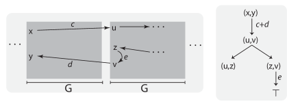
Figure 3: A path in a composition of $G$’s and the corresponding p-tree.

Definition 11

A p-tree is a weighted tree whose nodes are labelled with $\top$ or pairs of variables from $X$. Nodes labelled by $\top$ are leaves. A node labelled by a pair of variables $(x,y)$ can have one or two children as given in Figure 4.

Figure 4: Possible children of $(x,y)$ in a p-tree

The weight of a p-tree is the sum of weights that appear in it. A $p$-tree is complete if all the leaves are labelled by $\top$.

An $(x,y)$-$(u,v)$ context is a p-tree with the root labelled $(x,y)$ and all the leaves labelled $\top$ except for one leaf that is labelled $(u,v)$.

The definition of p-tree reflects the fact that each time the path can either go to the left or to the right, or stay in the same column. Every p-tree represents a path in an $i$-fold composition $(G_{\sigma})^{i}$ and every path in $(G_{\sigma})^{i}$ can be seen as a p-tree.

Lemma 12

Take an $i\in\{1,2,\dots\}$ and consider an $i$-fold composition of $G_{\sigma}$. For every pair of vertices $(j,x)$ to $(j,y)$ in the same column of $G_{\sigma}^{i}$: if there is a path of weight $w$ from $(j,x)$ to $(j,y)$ then there is a complete p-tree of weight $w$ with the root labeled $(x,y)$.

Proof.

Consider a path $\pi$ from $(j,x)$ to $(j,y)$. We construct its p-tree by an induction on the length of $\pi$. If $\pi$ is just an edge $(j,x)\xrightarrow{~{}e~{}}(j,y)$, then the corresponding p-tree would have $(x,y)$ as root and a single child labeled $\top$. The weight of the edge would be $e$.

Suppose $\pi$ is a sequence of edges. We make the following division based on its shape.

Case 1:

The path $\pi$ could cross the $j^{th}$ column at some vertex $(j,z)$ before reaching $(j,y)$: $(j,x)\xrightarrow{}\cdots\xrightarrow{}(j,z)\xrightarrow{}\cdots\xrightarrow{}(j,y)$. By induction, there are complete p-trees for the paths $(j,x)\xrightarrow{}\cdots(j,z)$ and $(j,z)\xrightarrow{}\dots(j,y)$. The p-tree for $\pi$ would have $(x,y)$ as root and $(x,z)$ and $(z,y)$ as its two children. The edge weights to the two children would be $(\leq,0)$. The p-trees of the smaller paths would be rooted at $(x,z)$ and $(z,y)$.

Case 2:

The path $\pi$ never crosses the $j^{th}$ column before reaching $(j,y)$. This means the path is entirely to either the left or right of the $j^{th}$ column. Let us assume it is to the right. The case for left is similar. So $\pi$ looks like: $(j,x)\xrightarrow{c}(j+1,u)\cdots(j+1,v)\xrightarrow{d}(j,y)$. Note that $u$ cannot be equal to $v$ since the path of the minimal weight must be simple (in the case when the path has exactly three nodes $(j,x),(j+1,v),(j,y)$, there is actually a direct edge from $(j,x)$ to $(j,y)$, as $|G_{\sigma}|$ is in the canonical form). By induction, the smaller path segment from $(j+1,u)$ to $(j+1,v)$ has a p-tree. The p-tree for $\pi$ would have $(x,y)$ as root and a single child $(u,v)$. The weight of this edge would be $c+d$. The p-tree for the smaller path would be rooted at $(u,v)$. ∎

Lemma 13

If there is a complete p-tree with the root $(x,y)$, weight $w$ and height $k$ then in $G_{\sigma}^{2k}$ the weight of the shortest path from $(k,x)$ to $(k,y)$ is at most $w$.

Proof.

For every level moved down in the p-tree, the corresponding path either moves one column left or one column right. As the height of the p-tree is bounded by $k$, there is a path that spans less than $k$ columns. This path goes from $(k,x)$ to $(k,y)$ in the composition $G_{\sigma}^{2k}$. Its weight is the weight of the tree. Therefore the smallest weight of a path from $(k,x)$ to $(k,y)$ is at most $w$. ∎

Now that we have established the correspondence between paths and p-trees, we are in a position to define a pattern in the paths that causes non-iterability.

Definition 12

A pattern is an $(x,y)$-$(x,y)$ context for some variables $x$ and $y$, whose weight is negative (c.f. Figure 5). We say that $\sigma$ admits a pattern if there is a pattern (notice that the definition of p-tree depends on $\sigma$).

Figure 5: Pattern: root is $(x,y)$ and the only leaf that is not $\top$ is $(x,y)$ again. Moreover, the weight has to be negative.

The next proposition says that patterns characterize $\omega$-iterability. Morever, it ensures that we can conclude after $n^{2}$ iterations. For transformation graphs $G_{1},G_{2}$, we will write $G_{1}\bumpeq G_{2}$ if $\mathit{left}(G_{1})=\mathit{left}(G_{2})$ and $\mathit{right}(G_{1})=\mathit{right}(G_{2})$.

Proposition 2

If $\sigma$ admits a pattern then there is no valuation from which $\sigma$ is $\omega$-iterable. If $\sigma$ does not admit a pattern, then for every $i=1,2\dots$ we have $(G_{\sigma})^{n^{2}}\bumpeq(G_{\sigma})^{n^{2}+i}$.

Proof of the above proposition follows from Lemmas 14, 15, 16.

Lemma 14

If $\sigma$ admits a pattern then there is no valuation from which $\sigma$ is $\omega$-iteratable.

Proof.

We will show that there is $k$ such that there is a negative cycle in the $k$-th fold composition $G_{\sigma}\odot\cdots\odot G_{\sigma}$.

Suppose $\sigma$ admits a pattern. Suppose we have clocks $x,y$ such that $x\leq y$ is implied by $\sigma$. This means that the last reset of $y$ happens before the last reset of $x$ in $\sigma$. In consequence $x\leq y$ is an invariant at the end of every iteration of $\sigma$.

Consider a sufficiently long composition $G_{\sigma}\odot\cdots\odot G_{\sigma}$. Since there is a pattern, for some $i<j$ we have one of the two cases

1. there is a path $(i,x)$ to $(j,x)$ and from $(j,y)$ to $(i,y)$ whose sum of weights is negative.

2. there is a path $(j,x)$ to $(i,x)$ and from $(i,y)$ to $(j,y)$ whose sum of weights is negative.

Observe that since $x\leq y$, we have an edge of weight at most $(\leq,0)$ from $y$ to $x$ in every iteration.

The case 1 makes the edge $y\to x$ more and more negative when going to the right. The case 2 makes the leftmost edge $x\leq y$ more and more negative depending on the number of iterations.

The second case clearly implies that an infinite iteration is impossible: in every valuation permitting $\omega$-iteration the distance from $x$ to $y$ would need to be infinity.

The first case tells that in subsequent iterations the difference between $x$ and $y$ should grow. Since every variable is reset in every iteration, this implies that the amount of time elapsed in each iteration should grow too. But this is impossible since, as we will show in the next paragraph, the presence of the edge $(j,y)$ to $(i,y)$ of weight $d$ implies that the value of $y$ after each execution of $\sigma$ is bounded by $d$. In consequence the difference between $x$ and $y$ is bounded too. A contradiction.

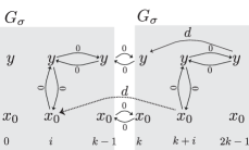
Figure 6: An edge from $(2,y)$ to $(1,y)$ gives a bound on time elapse

It remains to see why the edge $(j,y)$ to $(i,y)$ of weight $d$ implies that the value of $y$ at the end of each iteration of $\sigma$ is bounded. For simplicity of notation take $j=1$ and $i=2$, the argument is the same for other values. We will show that the last two resets of $y$ in the consecutive executions of $\sigma$ need to happen in not more than $d$ time units apart. This implies that the value of $y$ is bounded by $d$.

In Figure 6 we have pictured the composition of two copies of the transition graph $G_{\sigma}$. The graph has $k$ columns: numbered from $0$ to $k-1$. The last reset of $y$ is in the column $i$, so in the second copy it is in the column $k+i$. The black edges with weight $0$ come from the definition of the transition graph. For example the horizontal weight $0$ edges between $y$’s are due to the fact that $y$ is not reset between columns $i$ and $k-1$. As we can see from the picture, the edge of weight $d$ from $(k,y)$ and $(2k+1,y)$ induces an edge of weight $d$ from $(k+i,x_{0})$ to $(i,x_{0})$. Take a valuation $v$ satisfying the pictured composition of the two graphs $G_{\sigma}$. The induced edge gives us $v(i,x_{0})-v(k+i,x_{0})\leq d$. Recall that the value $-v(i,x_{0})$ represents the time instance when the column $i$ “happens”. Rewriting the last inequality as $(-v(k+i,x_{0}))-(-v(i,x_{0}))\leq d$, we can see that between columns $i$ and $k+i$ at most $d$ units of time have passed. So the value $v(k-1,y)-v(k-1,x_{0})$, that is the value of $y$ at the end of the first iteration of $\sigma$ is bounded by $d$.∎∎

The above lemma says that if there is a pattern, then $\sigma$ cannot be iterated. We will now show that if there is no pattern, then the p-trees representing shortest paths are bounded by $n^{2}$ and hence $n^{2}$ iterations will be sufficient to conclude if the sequence is $\omega$-iterable.

Lemma 15

If $\sigma$ does not admit a pattern then for every $(x,y)$ there is a complete p-tree of minimal weight and height bounded by $n^{2}$ whose root is $(x,y)$.

Proof.

In order to get a p-tree with minimal weight, observe that if we have a repetition of a label in the tree then we can cut out the part of the tree between the two repetitions. Moreover, we know that this part of the tree would sum up to a non-negative weight as by assumption $\sigma$ does not have a pattern. Therefore, cutting out the part between repetitions gives another tree that has smaller height and does not have a bigger weight. The height of a p-tree with no repetitions is bounded by $n^{2}$. ∎

Lemma 16

If $\sigma$ does not admit a pattern, then for every $i=1,2\dots$ we have $G_{\sigma}^{n^{2}+i}\bumpeq G_{\sigma}^{n^{2}}$.

Proof.

Due to Lemma 15, the shortest paths between any two variables in the leftmost column does not cross $n^{2}$ columns. Similarly the shortest path between any two variables in the rightmost column cannot go more than $n^{2}$ columns to the left. As this value is the same for both $G_{\sigma}^{n^{2}}$ and $G_{\sigma}^{n^{2}+i}$, the lemma follows. ∎∎

Based on Proposition 1, we get a procedure for checking if $\sigma$ is $\omega$-iterable.

Theorem 4.1

Let $\sigma$ be a sequence of transitions and let $n$ be the number of clocks. Following is a procedure for checking if $\sigma$ is $\omega$-iterable.

1. If $\sigma$ satisfies Lemma 2, report $\sigma$ is not $\omega$-iterable. Otherwise, continue.

2. If there is no clock that is both reset and is checked for $\succcurlyeq c$ with $c>0$ in some guard, report $\sigma$ is iterable. If there is such a clock, remove from $\sigma$ all guards containing clocks that are not reset and continue.

3. Compute $G^{1}=G_{\sigma}$; stop if it defines the empty relation.

4. Iteratively compute $G^{2^{k+1}}=G^{2^{k}}\cdot G^{2^{k}}$; stop if the result defines the empty relation, or $2^{k}>n^{2}$, or $G^{2^{k+1}}\bumpeq G^{2^{k}}$.

If a result is not defined or $2^{k}>n^{2}$ then $\sigma$ is not $\omega$-iterable. If $G^{2^{k+1}}=G^{2^{k}}$ then $\mathit{left}(G^{2^{k}})$ is the zone consisting precisely of all the valuations from which $\sigma$ is $\omega$-iterable.

Proof.

The first two steps are justified by Proposition 1. We discuss the third and fourth steps.

If at some moment the result of an operation is not defined then there is a negative cycle in $G^{2^{k}}_{\sigma}$, so $\sigma$ can be executed not more than $2^{k}$ times. Hence $\sigma$ is not $\omega$-iteratable.

If $2^{k}>n^{2}$ then there is a pattern and $\sigma$ is not $\omega$-iteratable (c.f. Lemma 16).

If $G^{2^{k+1}}=G^{2^{k}}$, then it means that the left column will not change on further compositions. As $G_{\sigma}$ is the graph that reflects $\sigma$, we have that $\mathit{left}(G^{2^{k}})$ is the set of valuations from which $\sigma$ is $\omega$-iteratable. ∎

∎

Complexity of this procedure is $\mathcal{O}((|\sigma|+\log n)\cdot n^{3})$. The graph $G_{\sigma}$ is build by incremental composition of the transitions in $\sigma$. Each transition in $\sigma$ can be encoded as a transformation graph over $2n$ variables. The sequential composition of two transformation graphs over $2n$ variables uses a DBM over $3n$ variables (with $n$ variables shared by the two graphs). The canonicalization of this DBM is achieved in time $(3n)^{3}$ and yields a transformation graph over $2n$ variables corresponding to the composition of the relations. Hence, $G_{\sigma}$ is obtained in time $\mathcal{O}(2|\sigma|\cdot(3n)^{3})$ assuming that each step in $\sigma$ corresponds to a transition followed by a delay. Once $G_{\sigma}$ has been computed, $(G_{\sigma})^{n^{2}}$ is obtained in time $\mathcal{O}(2\log n\cdot(3n^{3}))$ using the fact that $(G_{s})^{2k}=(G_{s})^{k}\cdot(G_{s})^{k}$ for $k\geq 1$.

5 Experiments

In this section we give some indications about the usefulness of the $\omega$-iterability check. The example from page 1 shows that the gains from our $\omega$-iteration procedure can be arbitrarily big. Still, it is more interesting to see the performance of $\omega$-iterability check on standard benchmark models. For this we have taken the collection of the same standard models as in many other papers on the verification of timed systems and in particular in [21].

Our testing scheme is as follows: we will verify properties given by Büchi automata on the standard benchmarks. To do this, we take the product of the model and property automata and check for Büchi non-emptiness on this product automaton. Algorithms for the Büchi non-emptiness problem can broadly be classified into two kinds: nested DFS-based [20] and Tarjan-based decomposition into SCCs [11]. Both these algorithms are essentially extensions of the simple DFS algorithm with extra procedures that help identify cycles containing accepting states. Currently, no algorithm is known to outperform the rest in all cases [14].

Restricting to weak Büchi properties.

In order to focus on the influence of iterability checking we consider weak Büchi properties (all states in a cycle are either accepting or non-accepting). In this case, the simple modification of DFS is the undisputed best algorithm: to find an accepting loop, it is enough to look for it on the active path of the DFS [7]. In other words, it is nested DFS where the secondary DFS search is never started.

The algorithm, that we will call DFS with subsumption (DFSS), performs a classical depth-first search on the finite abstracted zone graph $ZG^{\mathsf{Extra}_{LU}^{+}}(\mathcal{A})$. It uses the additional information provided by the zones to limit the seach from the current node $(q^{\prime},Z^{\prime})$ in two cases: (1) if $q^{\prime}$ is accepting and on the stack there is a path $\sigma$ from a node $(q^{\prime},Z^{\prime\prime})$ to the current node with $Z^{\prime\prime}\subseteq Z^{\prime}$ then report existence of an accepting path; and (2) if there is a fully explored a node $(q^{\prime},Z^{\prime\prime})$, i.e a node not on the stack, with $Z^{\prime}\subseteq Z^{\prime\prime}$ then ignore the current node and return from the DFS call. This is the algorithm one obtains after specialisation of the algorithm of Laarman et al. [21] to weak Buchi properties. It is presented in full in Appendix 0.A.

Now, it is quite clear how to add $\omega$-iterability check to this algorithm. We extend case (1) above using $\omega$-iterability check. When $q^{\prime}$ is accepting but $Z^{\prime\prime}\not\subseteq Z^{\prime}$ we use $\omega$-iterability check on $\sigma$. If $\sigma$ is iterable from $(q^{\prime},Z^{\prime})$, we have detected an accepting path and we stop the search. We refer to this algorithm as iDFSS: DFSS with $\omega$-iteration testing. Notice that when iDFSS stops thanks to $\omega$-iteration check, DFSS would just continue its search. The algorithm is listed in Appendix 0.A.

Our aim is to test the gains of iDFSS over DFSS. One can immediately see that iDFSS is not better than DFSS if there is no accepting path. Therefore in our examples we consider only the cases when there is an accepting path, to see if iDFSS has an effect now.

We tried variants of properties from [21] on the standard models (TrainGate, Fischer, FDDI and CSMA/CD). The results were not very encouraging: $\omega$-iterability check was hardly ever used, and when used the gains were negligible. Based on a closer look at these timed models, we argue that while these models are representative for reachability checking, their structure is not well adapted to evaluate algorithms for Büchi properties. We explain this in more detail below.

A note on standard benchmarks.

In three out of four models (Fischer, TrainGate and CSMA/CD), on every loop there is a true zone (which is the zone representing the set of all possible valuations). Moreover, in Fischer and TrainGate, a big majority of configurations have true zones, and even more strikingly, the longest sequence of configurations with a zone other than true does not exceed the number of components in the system: for example, in Fisher-$3$ there are at most $3$ consecutive nontrivial zones. As we explain in the next paragraph, in the case of CSMA/CD all the loops turn out to be almost trivial. Thus in all the three models one can as well ignore timing information for loop detection: it is enough to look at configurations with the true zone. This analysis explains the conclusion from [21] where it is reported that checking for counterexamples is almost instantaneous. Indeed, checking for simple untimed weak Büchi properties on these models will be very fast since every repetition of a state $q$ of the automaton will give a loop that is $\omega$-iteratable in $ZG^{\mathsf{Extra}_{LU}^{+}}(\mathcal{A})$. This loop will be successfully detected by the inclusion test (1) in DFSS algorithm since both zones will be true. The fourth model from standard benchmarks - FDDI - is also very peculiar. In this paper we are using $\mathsf{Extra}_{LU}^{+}$ abstraction for easy of comparison. Yet more powerful abstractions allow to eliminate time component completely from the model [19]. This indicates that dependencies between clocks in the model are quite weak.

Figure 7: Model of the CSMA/CD protocol: station (left) and bus (right).

The case of CSMA/CD gives an interesting motivation for testing Büchi properties. CSMA/CD is a protocol used to communicate over a bus where multiple stations may emit at the same time. As a result, message collisions may occur and have to be detected. Figure 7 shows a model for this protocol. We assume that the stations and the bus synchronize on actions. In particular, the transition from state $COLLISION$ to state $IDLE$ in the bus automaton synchronizes on action $cd_{i}$ in all $N$ stations. The model is parametrized by the propagation delay $S$ on the bus and the time $L$ needed to transmit a message which are usually set to $L=808$ and $S=26$ [24, 25].

It turns out that the $busy_{i}$ loop on state $RETRY$ in the station automaton is missing in the widely used model [24, 25]. In consequence, in this model there is no execution with infinitely many collisions and completed emissions. Even more, once some process enters in a collision, no process can send a message afeterwards. This example confirms once more that timed models are compact descriptions of complicated behaviours due to both parallelism and interaction between clocks. Büchi properties can be extremely useful in making sure that a model works as intended: the missing behaviors can be detected by checking if there is a run where every collision is followed by an emission. Adding the $busy_{i}$ loop on state $RETRY$ enables interesting behaviours where the stations have collisions and then they restart sending messages. The resulting model has significantly more reachable states and behaviours (see Appendix 0.B).

The other issue with CSMA/CD is that it has Zeno behaviours, and they appear precisely in the interesting part concerning collision. A solution we propose is to enforce $(y\geq 1)$ on all transitions from state $BUSY$ in the bus automaton. By chance, the modified model does not have new reachable states. But of course now all loops are nonZeno.

To sum up the above discussion, due to the form of the benchmark models, we are lead to consider Büchi properties that refer to time. This gives us a product automaton having zones with non-trivial interplay of clocks, and consequently making the Büchi non-emptiness problem all the more challenging. Figure 8 (right) presents the property we have checked on the modified CSMA/CD model. It checks if station $1$ can try to transmit fast enough, and if it arrives to send a message, the delay is not too long. The properties we have considered for other models are listed in Appendix 0.B. An important point is that since the exploration ends as soon as it finds a loop, the order of exploration influences the results. For fairnesss of the comparison we have run numerous times the two algorithms using random exploration order, both algorithms following the same order each time. The results of the experiments are presented in Figure 8 (left). All the examples have an accepting run.

Bottomline.

The table shows that there are quite natural properties of standard timed models where the use of $\omega$-iteration makes a big difference. Of course, there are other examples where $\omega$-iteration contributes nothing. Yet, when it gives nothing, $\omega$-iteration will also not cost much because it will not be called often.

Model DFSS algorithm iDFSS algorithm Visited nodes Visited nodes Iterability checks Mean Min Max Mean Min Max Mean Min Max CSMA/CD 4 9956 9699 10862 137 8 1646 1 1 1 CSMA/CD 5 12108 11315 14433 219 9 1331 1 1 1 CSMA/CD 6 16284 12931 25861 561 10 3523 1 1 1 Fischer 3 1067 275 9638 294 7 1625 3 1 28 Fischer 4 6516 365 129211 1284 7 21806 12 1 1296 Fischer 5 91124 455 1171755 17402 7 352682 30 1 1131 FDDI 8 4807 1489 11778 1652 1105 4022 23 1 71 FDDI 9 6326 2544 19046 1979 1247 11514 24 1 73 FDDI 10 7156 2840 25705 2101 1390 11587 22 1 65 Train Gate 3 1017 212 3649 109 4 528 1 1 1 Train Gate 4 14928 281 65358 1874 4 11844 3 1 90 Train Gate 5 448662 350 1243873 63000 4 235957 29 1 397

Figure 8: Benchmarks (left) and property checked on CSMA/CD (right).

6 Conclusions

We have presented a method for testing $\omega$-iterability of a cycle in a timed automaton. Concentrating on iterability, as opposed to loop decomposition [9], has allowed us to obtain a relatively efficient procedure, with a complexity comparable to zone canonicalisation. We have performed experiments on the usefulness of this procedure for testing weak Büchi properties of standard benchmark models. This has led us to examine in depth the structure of these models. This structure explains why testing untimed Büchi properties turned out to be immediate. When we have tested for timed Büchi properties the situation changed completely, and we could observe substantial gains on some examples.

There is no particular difficulty in integrating our $\omega$-iterability test in a tool for checking all Büchi properties. Due to the lack of space we have chosen not to report on the prototype here. Let us just mention that we prefer methods based on Tarjan’s strongly connected components since they adapt to multi Büchi properties, and allow to handle Zeno issues in a much more effective way than strongly non-Zeno construction [17].

Although efficient in some cases, $\omega$-iterability test does not solve all the problems of testing Büchi properties of timed automata. In particular when there is no accepting loop in the automaton, the test brings nothing, and one can often observe a quick state blowup. New ideas are very much needed here.

Appendix 0.A DFSS and iDFSS algorithms

Listing 1: iDFSS algorithm.

⬇

1procedure iDFSS($\mathcal{A}=(Q,q_{0},X,T,F)$)

2 Cyan:=Blue:=$\emptyset$;

3 explore($(q_{0},Z_{0})$);

4 report no cycle;

5

6procedure explore($(q,Z)$)

7 Cyan:=Cyan$\,\cup\,\{(q,Z)\}$;

8 for all $(q^{\prime},Z^{\prime})\in\mathsf{POST}((q,Z))$ do

9 if $q^{\prime}\not\in F$ and $(q^{\prime},Z^{\prime})\in Cyan$ then

10 skip //ignore $(q^{\prime},Z^{\prime})$

11 if $q^{\prime}\in F$ then

12 if $\exists(q^{\prime},Z^{\prime\prime})\in Cyan.\ Z^{\prime\prime}\subseteq Z^{\prime}$ then report cycle;

13 if $\exists(q^{\prime},Z^{\prime\prime})\in Cyan$ then

14 let $\sigma$ be the path $(q^{\prime},Z^{\prime\prime})\to(q^{\prime},Z^{\prime})$ on the stack;

15 if $\omega$-iterable($\sigma$) then report cycle;

16 if $\exists(q^{\prime},Z^{\prime\prime})\in Blue.\ Z^{\prime}\subseteq Z^{\prime\prime}$ then

17 skip //ignore $(q^{\prime},Z^{\prime})$

18 else

19 explore($(q^{\prime},Z^{\prime})$);

20 Blue:=Blue$\,\cup\,\{(q,Z)\}$;

21 Cyan:=Cyan$\,\setminus\,\{(q,Z)\}$;

Algorithm iDFSS is presented in Listing 1. This algorithm runs a depth-first search over the finite abstracted zone graph $ZG^{\mathsf{Extra}_{LU}^{+}}(\mathcal{A})$ of a timed Büchi automaton $\mathcal{A}$ to check whether $\mathcal{A}$ has an accepting run. To that purpose, the algorithm maintains two sets of states. $Blue$ contains fully visited states and $Cyan$ consists in partially visited states that form the current search path.

Algorithm iDFSS uses the information provided by the zones to limit the seach from the current node $(q^{\prime},Z^{\prime})$ in three cases:

1. if $q^{\prime}$ is accepting and on the stack there is a path $\sigma$ from a node $(q^{\prime},Z^{\prime\prime})$ to the current node with $Z^{\prime\prime}\subseteq Z^{\prime}$ then report existence of an accepting path (line 12).

2. when $q^{\prime}$ is accepting but $Z^{\prime\prime}\not\subseteq Z^{\prime}$ we use $\omega$-iterability check on $\sigma$. If $\sigma$ is iterable from $(q^{\prime},Z^{\prime})$, we have detected an accepting path and we stop the search (line 13).

3. if there is a fully explored a node $(q^{\prime},Z^{\prime\prime})$, i.e a node not on the stack, with $Z^{\prime}\subseteq Z^{\prime\prime}$ then ignore the current node and return from the DFS call (line 16).

In this paper, we compare algorithm iDFSS to algorithm DFSS that does not use iterability check (i.e. with line 13 and the next two lines removed). This is the algorithm one obtains after specialisation of the algorithm of Laarman et al. [21] to weak Buchi properties.

Appendix 0.B Models and properties

In our experiments we have used the following models:

• Train gate controller [1, 2]

• Fischer’s Mutex protocol [3, 4]

• CSMA/CD [3, 5]

• FDDI [6, 7]

The above models have been used as benchmarks to evaluate algorithms for safety and liveness [8, 9]. As we have explained in the main text the standard benchmark CSMA/CD model has a transition missing. In Figure 9 we graphically represent the model with 3 stations, the new behaviours due to adding the missing transition are marked in red. The intention of this figure is just to give a visual impression of what is the influence of the added transition. After adding the transition there are no new states, but there are new behaviours.

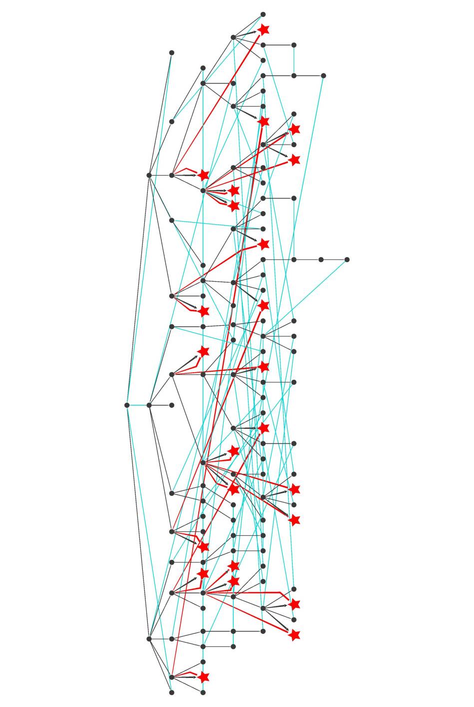
Figure 9: CSMA/CD model: after correcting the model we obtain new cycles marked in red.

Figure 10: Property for model Fischer with $N$ processes and $T=K*N$. The automaton checks if the first process can request fast, and can only enter the critical section after a certain amount of time and before timeout.

Figure 11: Property for model FDDI with $N=3$ stations and $U=150*SA*N$. The automaton checks if all stations can send asynchronous messages in the same round infinitely often and in a bounded amount of time.

Figure 12: Property for model Train Gate, with $N$ trains. The automaton checks if Train $1$ can approach frequently fast but hardly waits for other trains.

References

- [1] R. Alur and D.L. Dill. A theory of timed automata. Theoretical Computer Science, 126(2):183–235, 1994.
- [2] G. Behrmann. Distributed reachability analysis in timed automata. STTT, 7(1):19–30, 2005.
- [3] G. Behrmann, P. Bouyer, K. G. Larsen, and R. Pelánek. Lower and upper bounds in zone-based abstractions of timed automata. STTT, 8(3):204–215, 2006.
- [4] B. Boigelot and F. Herbreteau. The power of hybrid acceleration. In CAV, volume 4144 of LNCS, pages 438–451, 2006.
- [5] M. Bozga, R. Iosif, and F. Konečný. Deciding conditional termination. In TACAS, volume 7214 of LNCS, pages 252–266, 2012.
- [6] M. Bozga, R.Iosif, and Y. Lakhnech. Flat parametric counter automata. In ICALP, volume 4052 of LNCS, pages 577–588, 2006.
- [7] I. Cerná and R. Pelánek. Relating hierarchy of temporal properties to model checking. In MFCS, volume 2747 of LNCS, pages 318–327, 2003.
- [8] H. Comon and Y. Jurski. Multiple counters automata, safety analysis and presburger arithmetic. In CAV, volume 1427 of LNCS, pages 268–279, 1998.
- [9] H. Comon and Y. Jurski. Timed automata and the theory of real numbers. In CONCUR, volume 1664 of LNCS, pages 242–257, 1999.
- [10] B. Cook, S. Gulwani, T. Lev-Ami, A. Rybalchenko, and M. Sagiv. Proving conditional termination. In CAV, volume 5123 of LNCS, pages 328–340, 2008.
- [11] J.-M. Couvreur. On-the-fly verification of linear temporal logic. In FM, volume 1708 of LNCS, pages 253–271, 1999.
- [12] C. Daws and S. Tripakis. Model checking of real-time reachability properties using abstractions. In TACAS, volume 1384 of LNCS, pages 313–329, 1998.
- [13] D. L. Dill. Timing assumptions and verification of finite-state concurrent systems. In Automatic Verification Methods for Finite State Systems, pages 197–212, 1989.
- [14] A. Gaiser and S. Schwoon. Comparison of algorithms for checking emptiness on Büchi automata. In MEMICS, volume 13 of OASICS, pages 69–77, 2009.
- [15] A. Gupta, T. A. Henzinger, R. Majumdar, A. Rybalchenko, and Ru-Gang Xu. Proving non-termination. In POPL, pages 147–158. ACM, 2008.
- [16] F. Herbreteau, D. Kini, B. Srivathsan, and I. Walukiewicz. Using non-convex approximations for efficient analysis of timed automata. CoRR, abs/1110.3704, 2011.
- [17] F. Herbreteau and B Srivathsan. Efficient on-the-fly emptiness check for timed büchi automata. In ATVA, pages 218–232. Springer, 2010.
- [18] F. Herbreteau, B Srivathsan, and I. Walukiewicz. Better abstractions for timed automata. In LICS, pages 375–384. IEEE Computer Society, 2012.
- [19] F. Herbreteau, B. Srivathsan, and I. Walukiewicz. Lazy abstractions for timed automata. In CAV, volume 8044 of LNCS, pages 990–1005, 2013.
- [20] G. J. Holzmann, D. Peled, and M. Yannakakis. On nested depth first search. DIMACS Series in Discrete Mathematics and Theoretical Computer Science, 32:23–31, 1997.
- [21] A. Laarman, Olesen M. C., Dalsgaard A. E., Larsen K. G., and J. van de Pol. Multi-core emptiness checking of timed büchi automata using inclusion abstraction. In CAV, volume 8044 of LNCS, pages 968–983, 2013.
- [22] G. Li. Checking timed Büchi automata emptiness using LU-abstractions. In FORMATS, pages 228–242, 2009.
- [23] A. Tiwari. Termination of linear programs. In CAV, volume 3114 of LNCS, pages 70–82, 2004.
- [24] S. Tripakis and S. Yovine. Analysis of timed systems using time-abstracting bisimulations. Formal Methods in System Design, 18(1):25–68, 2001.
- [25] UPPAAL CSMA/CD model. http://www.it.uu.se/research/group/darts/uppaal/benchmarks/genCSMA_CD.awk. Accessed: 2014-10-08.

References

- [1] W. Yi and P. Pettersson and M. Daniels. Automatic verification of real-time communicating systems by constraint-solving In FORTE, volume 6 of IFIP Conference Proceedings, pages 243–258, 1994.
- [2] UPPAAL Train Gate model. Provided with UPPAAL model-checker: http://www.uppaal.org. Accessed: 2014-10-08
- [3] S. Tripakis and S. Yovine. Analysis of Timed Systems Using Time-Abstracting Bisimulations. Formal Methods in System Design, 18(1):25–68, 2001
- [4] UPPAAL Fischer’s Mutex model. http://www.it.uu.se/research/group/darts/uppaal/benchmarks/genFischer.awk, Accessed: 2014-10-08
- [5] UPPAAL CSMA/CD model. http://www.it.uu.se/research/group/darts/uppaal/benchmarks/genCSMA_CD.awk, Accessed: 2014-10-08
- [6] C. Daws and A. Olivero and S. Tripakis and S. Yovine. The tool KRONOS, in Hybrid Systems III, volume 1066 of LNCS, pages 208–219, 1996.
- [7] UPPAAL Token ring FDDI protocol model. http://www.it.uu.se/research/group/darts/uppaal/benchmarks/genHDDI.awk, Accessed: 2014-10-08
- [8] F. Herbreteau and B. Srivathsan and I. Walukiewicz. Lazy Abstractions for Timed Automata. In CAV, volume 8044 of LNCS, pages 990–1005, 2013.
- [9] A. Laarman and M. C., Olesen and A. E., Dalsgaard and K. G., Larsen and J. van de Pol. Multi-core emptiness checking of timed Büchi automata using inclusion abstraction In CAV, volume 8044 of LNCS, pages 968–983, 2013.