Functionally fitted
Runge-Kutta-Nyström methods

Abstract.

We have shown previously that functionally fitted Runge-Kutta (FRK) methods can be studied using a convenient collocation framework. Here, we extend that framework to functionally fitted Runge-Kutta-Nyström (FRKN) methods, shedding further light on the fact that these methods can integrate a second-order differential equation exactly if its solution is a combination of certain basis functions, and that superconvergence can be obtained when the collocation points satisfy some orthogonality conditions. An analysis of their stability is also conducted.

1. Introduction

Consider the special second-order differential equation

(1.1) $$\begin{split}y&{}^{\prime\prime}(t)=f(t,y(t)),\quad y(t_{0})=y_{0},\quad y^{\prime}(t_{0})=y^{\prime}_{0},\\ y&:{\mathbb{R}}\rightarrow{\mathbb{R}},\quad f:{\mathbb{R}}\times{\mathbb{R}}\rightarrow{\mathbb{R}},\quad t\in[t_{0},\,t_{0}+T],\end{split}$$

where, for simplicity of notation, we keep (1.1) in scalar form although our results apply to a system of ODEs as well. We assume that the problem satisfies the necessary conditions to have a unique solution. Letting $z(t):=y^{\prime}(t)$, it is well known that this problem can be converted to a first-order IVP

(1.2) $$\begin{pmatrix}y(t)\\ z(t)\end{pmatrix}^{\prime}=\begin{pmatrix}z(t)\\ f(t,y(t))\end{pmatrix},\quad\begin{pmatrix}y(t_{0})\\ z(t_{0})\end{pmatrix}=\begin{pmatrix}y_{0}\\ y_{0}^{\prime}\end{pmatrix},$$

so that it can be studied entirely through this commonly called indirect approach. What is however preferable is to address (1.1) directly without doubling the dimension of the problem and/or introducing the term $y^{\prime}(t)$ that is not present in the initial problem. This is the popular approach taken by direct Runge-Kutta-Nyström (RKN) methods.

In [5, 6], we developed a collocation framework for functionally fitted Runge-Kutta (FRK) methods that can be applied to the indirect approach (1.2). We briefly alluded in [6, Remark 4.2] to a P-stability result adapted from this first-order formulation. But the prominence of direct RKN methods motivates recasting our framework to this popular and well-regarded setting. Consequently in this paper we target the special second-order IVP (1.1) as RKN methods do, and we develop functionally fitted Runge-Kutta-Nyström (FRKN) methods in a way that mirrors what we did for FRK methods. Although there are similarities with our previous work, this study fills a gap in the literature by providing a unifying umbrella for both FRK and FRKN methods. In a sense, similarities with [5, 6] validate our unified framework, but there are nevertheless differences in the details to make the most of the special form (1.1). The overlap is kept to a minimum by not repeating proofs that do not add a distinctive value to our presentation and that can be drawn from our earlier work, with hints given to the interested reader on how to recover them.

Among the many studies that have already been devoted to (1.1) other than general purpose methods, we can cite exponentially fitted methods [2, 3, 4, 8], and especially the work of Ozawa [7] who studied functionally fitted methods using Taylor series. Our paper builds on that work but uses collocation techniques. The organization of the paper is as follows. Section 2 formally defines functionally fitted Runge-Kutta-Nyström methods for general basis functions. Section 3 summarizes properties that arise from basis functions that are separable. Section 4 derives their order of accuracy using our collocation framework. Section 5 presents new results regarding their stability. Section 6 is a walk-through example. Section 7 provides some concluding remark.

2. Functionally fitted RKN methods

Recall that a conventional $s$-stage RKN method is often defined by its Butcher-tableau as

$$\begin{array}[]{c|c}\bm{c}&\bm{A}\\ \hline\cr&\bm{b}^{T}\\ &\bm{d}^{T}\end{array},~{}~{}\bm{A}=[a_{ij}]\in{\mathbb{R}}^{s\times s},~{}~{}\bm{b}=(b_{1},\ldots,b_{s})^{T},~{}~{}\bm{d}=(d_{1},\ldots,d_{s})^{T}.$$

For an explicit RKN method, the matrix $\bm{A}$ is strictly lower triangular and $c_{1}=0$. Let $\bm{e}=(1,\ldots,1)^{T}$ of length $s$, denote ${y}_{n}$ and ${y}^{\prime}_{n}$ the approximations to ${y}(t)$ and ${y}^{\prime}(t)$ at $t_{n}$, then the next iterates ${y}_{n+1}$ and ${y}^{\prime}_{n+1}$ are computed using

(2.1) $$y_{n+1} =y_{n}+hy^{\prime}_{n}+h^{2}\bm{b}^{T}f(\bm{e}t_{n}+\bm{c}h,\bm{Y}_{n})\in{\mathbb{R}},$$

(2.2) $$y^{\prime}_{n+1} =y^{\prime}_{n}+h\bm{d}^{T}f(\bm{e}t_{n}+\bm{c}h,\bm{Y}_{n})\in{\mathbb{R}},$$

(2.3) $$\bm{Y}_{n} =\bm{e}y_{n}+\bm{c}hy^{\prime}_{n}+h^{2}\bm{A}f(\bm{e}t_{n}+\bm{c}h,\bm{Y}_{n})\in{\mathbb{R}}^{s},$$

where $\bm{Y}_{n}=(Y_{n,1},\ldots,Y_{n,s})^{T}$ is the vector of intermediate stage values and $f(\bm{e}t_{n}+\bm{c}h,\bm{Y}_{n})=(f(t_{n}+c_{1}h,Y_{n,1}),\ldots,f(t_{n}+c_{s}h,Y_{n,s}))^{T}$.

Now, assume we are given distinct parameters $(c_{i})_{i=1}^{s}$, usually in $[0,1]$, and a set of linearly independent basis functions $\{u_{k}(t)\}_{k=1}^{s}$ that should not include $\{1,t\}$. We will augment the set with $\{1,t\}$ to characterize FRKN methods later because any problem for which the solution is a linear combination of $\{1,t\}$ is always integrated exactly by FRKN (and RKN) methods, regardless of basis functions. In general, basis functions are typically chosen to exploit any information on the solution that general purpose methods do not. The linear independence is to avoid undue redundancy in the set by not including a function that is merely a linear combination of the others. Functionally fitted (or generalized collocation) RKN methods are defined to solve (1.1) exactly if its solution is a linear combination of the chosen functions (Ozawa [7]).

Definition 2.1 (Functionally fitted RKN method).

An $s$-stage RKN method is an FRKN (or a generalized collocation RKN) method with respect to the basis functions $\{u_{k}(t)\}_{k=1}^{s}$ if the following relations are satisfied for all $k=1,\ldots,s$:

(2.4) $$\begin{split}u_{k}(t+h)&=u_{k}(t)+hu_{k}^{\prime}(t)+h^{2}\bm{b}(t,h)^{T}u_{k}^{\prime\prime}(\bm{e}t+\bm{c}h),\\ u^{\prime}_{k}(t+h)&=u^{\prime}_{k}(t)+h\bm{d}(t,h)^{T}u_{k}^{\prime\prime}(\bm{e}t+\bm{c}h),\\ u_{k}(\bm{e}t+\bm{c}h)&=\bm{e}u_{k}(t)+h\bm{c}u^{\prime}_{k}(t)+h^{2}\bm{A}(t,h)u_{k}^{\prime\prime}(\bm{e}t+\bm{c}h).\end{split}$$

The underlying coefficients $\bm{A}(t,h)$, $\bm{b}(t,h)$ and $\bm{d}(t,h)$ are often determined by solving the linear system of algebraic equations arising from (2.4). When the basis functions are the monomials, classical algebraic collocation RKN methods [9] are recovered. It is clear that a solution to (2.4) may or may not exist depending on the choice of $\{u_{k}(t)\}_{k=1}^{s}$. To guarantee the existence of a solution we require that the basis functions satisfy the collocation condition defined below.

Definition 2.2 (Collocation condition for FRKN methods).

A set of sufficiently smooth functions $\{u_{1}(t),\ldots,$ $u_{s}(t)\}$ is said to satisfy the collocation condition for FRKN methods if the following matrices

$$\bm{E}(t,h) =\bigg{(}u_{1}(\bm{e}t+\bm{c}h)-u_{1}(\bm{e}t)-\bm{c}hu^{\prime}_{1}(t),\ldots,u_{s}(\bm{e}t+\bm{c}h)-u_{s}(\bm{e}t)-\bm{c}hu^{\prime}_{s}(t)\bigg{)},$$

$$\bm{F}(t,h) =\bigg{(}u_{1}^{\prime\prime}(\bm{e}t+\bm{c}h),u_{2}^{\prime\prime}(\bm{e}t+\bm{c}h),\ldots,u_{s}^{\prime\prime}(\bm{e}t+\bm{c}h)\bigg{)},$$

are both nonsingular almost everywhere with respect to $h$ on $[0,T]$ for any given $t$.

Remark 2.3.

Note that the last equation in (2.4) can be rewritten as

$$\bm{E}(t,h)=h^{2}\bm{A}(t,h)\bm{F}(t,h).$$

Hence the existence of the matrix $\bm{A}(t,h)$ is guaranteed if $\bm{F}(t,h)$ is nonsingular, as required in Definition 2.2. We shall see later that by also requiring $\bm{E}(t,h)$ to be nonsingular we ensure the existence of the so-called collocation solution. Requiring both $\bm{E}(t,h)$ and $\bm{F}(t,h)$ nonsingular makes $\bm{A}(t,h)$ nonsingular as well, leading to FRKN methods that are implicit. By allowing $\bm{A}(t,h)$ to be strictly lower triangulary (thus singular), Franco and Gòmez [4] obtained explicit exponentially fitted RKN methods.

Remark 2.4.

In [7], Ozawa used Taylor series expansions to prove that when given any set of functions $\{\varphi_{k}(t)\}_{k=1}^{s}$, if the Wronskian $W(\varphi_{1},\varphi_{2},\ldots,\varphi_{s})(t)\neq 0$, then the matrix $\bm{\Phi}(t,h)=\big{(}\varphi_{1}(\bm{e}t+\bm{c}h),\varphi_{2}(\bm{e}t+\bm{c}h),\ldots,\varphi_{s}(\bm{e}t+\bm{c}h)\big{)}$ is nonsingular for small $h>0$. We can therefore conclude that $\bm{F}(t,h)$ is nonsingular for $h$ sufficiently small if $W(u_{1}^{\prime\prime},u_{2}^{\prime\prime},\ldots,u_{s}^{\prime\prime})(t)\neq 0,\,\forall t\in[t_{0},\,t_{0}+T]$. Moreover, using the same Taylor series approach, we can see that

$$\bm{E}(t,h)=\bigg{(}\frac{(\bm{c}h)^{2}}{2!},\frac{(\bm{c}h)^{3}}{3!},\ldots,\frac{(\bm{c}h)^{s+1}}{(s+1)!}\bigg{)}W(u_{1}^{\prime\prime},u_{2}^{\prime\prime},\ldots,u_{s}^{\prime\prime})(t)+O(h^{s+2}),$$

so that $W(u_{1}^{\prime\prime},u_{2}^{\prime\prime},\ldots,u_{s}^{\prime\prime})(t)\neq 0,\forall t\in[t_{0},\,t_{0}+T]$ is a sufficient (but not necessary) condition for both $\mathop{\rm det}\bm{E}(t,h)\neq 0$ and $\mathop{\rm det}\bm{F}(t,h)\neq 0$ when $h$ is sufficiently small. Thus, our condition is less restrictive than the one in [7]. Indeed it is easily verified that the set $\{\sin(\omega t),\sin(2\omega t)\}$ does not satisfy Ozawa’s condition but satisfy our collocation condition.

The following is a direct result of the collocation condition in Definition 2.2.

Theorem 2.5.

The coefficients of a FRKN method based on a set of functions that satisfy the collocation condition are uniquely determined almost everywhere with respect to $h$ on the interval of integration.

As we did with FRK methods in [5, 6], our overarching contribution is to study the order of accuracy of FRKN methods without using order conditions. We do so by establishing the existence of a fundamental function that we call the collocation solution. We also use this function later to analyze the stability.

Choose $(c_{i})_{i=1}^{s}$ and consider a FRKN method $(\bm{c}$, $\bm{A}(t,h)$, $\bm{b}(t,h)$, $\bm{d}(t,h))$ based on a set of given basis functions $\{u_{k}\}_{k=1}^{s}$. Let

$$\bm{H}: =\text{Span}\{1,t,u_{1}(t),\ldots,u_{s}(t)\}$$

$$=\bigg{\{}v(t)\bigg{|}v(t)=\alpha_{0}+a_{0}t+\sum_{i=1}^{s}a_{i}u_{i}(t);\,\alpha_{0},a_{0},\ldots,a_{s}\in\mathbb{R}\bigg{\}}.$$

We call $u(t)$ the collocation solution if it is an element of $\bm{H}$ that satisfies equation (1.1) at the collocation points $(hc_{i})_{i=1}^{s}$, that is,

(2.5) $$u(t_{0})=y_{0},\quad u^{\prime}(t_{0})=y^{\prime}_{0},\quad u^{\prime\prime}(t_{0}+c_{i}h)=f(t_{0}+c_{i}h,u(t_{0}+c_{i}h)),$$

for $i=1,\ldots,s$. As it is well known, the collocation method consists in taking the numerical solution after one step as

(2.6) $$y_{1}=u(t_{0}+h),\quad y_{1}^{\prime}=u^{\prime}(t_{0}+h).$$

Since $u(t)$ is only defined implicitly, we must first guarantee its existence in our context as well.

Lemma 2.6.

Suppose that we are given $s+2$ values $y_{0},y^{\prime}_{0},y_{1},\ldots,y_{s}$ and the pair $(t_{0},h)$ is such that $\bm{E}(t_{0},h)$ is nonsingular, then there exists an interpolation function $\varphi\in\bm{H}$ such that $\varphi(t_{0})=y_{0}$, $\varphi^{\prime}(t_{0})=y^{\prime}_{0}$, and $\varphi(t_{0}+c_{i}h)=y_{i}$, $i=1,\ldots,s$.

Proof.

Any function $\varphi\in\bm{H}$ can be represented in the form

$$\varphi(t)=\alpha_{0}+a_{0}t+\sum_{i=1}^{s}a_{i}u_{i}(t).$$

Letting $t_{i}:=t_{0}+c_{i}h$, $i=1,\ldots,s$, the interpolation criteria can be stated therefore as

(2.7) $$\begin{pmatrix}1&t_{0}&u_{1}(t_{0})&u_{2}(t_{0})&\cdots&u_{s}(t_{0})\\ 0&1&u^{\prime}_{1}(t_{0})&u^{\prime}_{2}(t_{0})&\cdots&u^{\prime}_{s}(t_{0})\\ 1&t_{1}&u_{1}(t_{1})&u_{2}(t_{1})&\cdots&u_{s}(t_{1})\\ \vdots&\vdots&\vdots&\ddots&\vdots\\ 1&t_{s}&u_{1}(t_{s})&u_{2}(t_{s})&\cdots&u_{s}(t_{s})\end{pmatrix}\begin{pmatrix}\alpha_{0}\\ a_{0}\\ a_{1}\\ \vdots\\ a_{s}\end{pmatrix}=\begin{pmatrix}y_{0}\\ y^{\prime}_{0}\\ y_{1}\\ \vdots\\ y_{s}\end{pmatrix}.$$

For this equation to have a unique solution the matrix in the left-hand side must be nonsingular. Subtracting its first row from the third to the last row, we see that its determinant is

(2.8) $$\begin{vmatrix}1&u^{\prime}_{1}(t_{0})&u^{\prime}_{2}(t_{0})&\cdots&u^{\prime}_{s}(t_{0})\\ c_{1}h&u_{1}(t_{1})-u_{1}(t_{0})&u_{2}(t_{1})-u_{2}(t_{0})&\cdots&u_{s}(t_{1})-u_{s}(t_{0})\\ c_{2}h&u_{1}(t_{2})-u_{1}(t_{0})&u_{2}(t_{2})-u_{2}(t_{0})&\cdots&u_{s}(t_{2})-u_{s}(t_{0})\\ \vdots&\vdots&\vdots&\ddots&\vdots\\ c_{s}h&u_{1}(t_{s})-u_{1}(t_{0})&u_{2}(t_{s})-u_{2}(t_{0})&\cdots&u_{s}(t_{s})-u_{s}(t_{0})\end{vmatrix}.$$

Multiplying the first row in the determinant in (2.8) by $c_{i}h$ and subtracting it from the $(i+1)$-th row for $i=1,\ldots,s$, one concludes that this determinant is

$$\begin{vmatrix}u_{1}(t_{1})-u_{1}(t_{0})-c_{1}hu^{\prime}_{1}(t_{0})&\cdots&u_{s}(t_{1})-u_{s}(t_{0})-c_{1}hu^{\prime}_{s}(t_{0})\\ u_{1}(t_{2})-u_{1}(t_{0})-c_{2}hu^{\prime}_{1}(t_{0})&\cdots&u_{s}(t_{2})-u_{s}(t_{0})-c_{2}hu^{\prime}_{s}(t_{0})\\ \vdots&\ddots&\vdots\\ u_{1}(t_{s})-u_{1}(t_{0})-c_{s}hu^{\prime}_{1}(t_{0})&\cdots&u_{s}(t_{s})-u_{s}(t_{0})-c_{s}hu^{\prime}_{s}(t_{0})\end{vmatrix}=\mathop{\rm det}\bm{E}(t_{0},h).$$

Therefore, the solution to (2.7) is uniquely determined since $\bm{E}(t_{0},h)$ is assumed nonsingular under the collocation condition. ∎

Theorem 2.7.

The collocation method defined by (2.5) and (2.6) is equivalent to the $s$-stage FRKN method with coefficients $(\bm{c}$, $\bm{A}(t,h)$, $\bm{b}(t,h)$, $\bm{d}(t,h))$.

Proof.

Consider the equations we have to solve in an $s$-stage FRKN method

(2.9) $$Y_{i}=y_{0}+hc_{i}y^{\prime}_{0}+h^{2}\sum_{j=1}^{s}a_{ij}f(t_{0}+c_{j}h,Y_{j}),\quad i=1,\ldots,s.$$

Let $(\overline{Y}_{1},\ldots,\overline{Y}_{s})^{T}$ be the unique solution to the system of equations (2.9). (Using fixed-point iterations one can show that this solution does indeed exist for a sufficiently small $h>0$.) Lemma 2.6 ensures that there is an interpolation function $\varphi(t)\in\bm{H}$ such that $\varphi^{\prime}(t_{0})=y^{\prime}_{0}$, $\varphi(t_{0})=y_{0}$, and $\varphi(t_{0}+c_{i}h)=\overline{Y_{i}}$, $i=1,\ldots,s$. Hence $\varphi(t)$ satisfies

(2.10) $$\varphi(\bm{e}t_{0}+\bm{c}h)=\bm{e}\varphi(t_{0})+\bm{c}h\varphi^{\prime}(t_{0})+h^{2}\bm{A}(t_{0},h)f(\bm{e}t_{0}+\bm{c}h,\varphi(\bm{e}t_{0}+\bm{c}h)).$$

Since $\varphi(t)\in\bm{H}=\mathop{\rm Span}\{1,t,u_{1}(t),\ldots,u_{s}(t)\}$, we can write

$$\varphi(t)=\alpha_{0}+a_{0}t+\sum_{k=1}^{s}a_{k}u_{k}(t),\quad\varphi^{\prime}(t)=a_{0}+\sum_{k=1}^{s}a_{k}u_{k}^{\prime}(t),\quad\varphi^{\prime\prime}(t)=\sum_{k=1}^{s}a_{k}u_{k}^{\prime\prime}(t),$$

and since the definition of a FRKN method (2.4) means that

$$u_{k}(\bm{e}t_{0}+\bm{c}h)=\bm{e}u_{k}(t_{0})+\bm{c}hu^{\prime}_{k}(t_{0})+h^{2}\bm{A}(t_{0},h)u_{k}^{\prime\prime}(\bm{e}t_{0}+\bm{c}h),\quad k=1,\ldots,s,$$

we can obtain

(2.11) $$\varphi(\bm{e}t_{0}+\bm{c}h)=\bm{e}\varphi(t_{0})+\bm{c}h\varphi^{\prime}(t_{0})+h^{2}\bm{A}(t_{0},h)\varphi^{\prime\prime}(\bm{e}t_{0}+\bm{c}h).$$

Since $\bm{A}(t_{0},h)$ is nonsingular, equations (2.10) and (2.11) imply that

$$\varphi^{\prime\prime}(t_{0}+c_{i}h)=f(t_{0}+c_{i}h,\varphi(t_{0}+c_{i}h)),\qquad i=1,\ldots,s.$$

Therefore, if we choose $u(t)=\varphi(t)$, then $u(t)$ satisfies equality (2.5), which proves the theorem. ∎

Remark 2.8.

It follows from the proof of Theorem 2.7 that the existence of a solution to the system (2.9) implies the existence of the collocation solution $u(t)$. In other words, the collocation solution $u(t)$ exists and is unique for a given $h>0$ whenever the associated FRKN method is applicable. For a sufficiently small $h>0$, we pointed out in the proof of Theorem 2.7 that the solution to the system (2.9) exists and is unique, and so we can conclude that the collocation solution exists and is unique as well. Moreover, as an element of $\bm{H}$, it is a linear combination of the given basis functions $\{u_{k}(t)\}_{k=1}^{s}$ augmented with $\{1,t\}$.

3. Separable basis

It is clear from our discussion so far that the analysis of FRKN methods is complicated by the fact that they have variable coefficients that depend on $t$, $h$ and the basis functions in a non-trivial manner. In [5] and [6], we introduced the class of separable methods to overcome the difficult for FRK methods. Here we extend this notion to FRKN methods.

Definition 3.1 (Separable basis).

A set of linearly independent functions $\{u_{k}\}_{k=1}^{s}$ is said to be a separable basis for FRKN methods if $\bm{u}(t):=(1,t,u_{1}(t),\ldots,u_{s}(t))^{T}$ satisfies

(3.1) $$\bm{u}(t+h)=\mbox{\boldmath$\mathcal{F}$}(h)\bm{u}(t)=\mbox{\boldmath$\mathcal{F}$}(t)\bm{u}(h),\quad\forall t,h\in\mathbb{R},$$

where $\mbox{\boldmath$\mathcal{F}$}:\mathbb{R}\to\mathbb{R}^{(s+2)\times(s+2)}$ is a suitable matrix function.

FRKN methods corresponding to separable bases are called separable methods. The following results characterize these methods further. Theorem 3.2 gives an indication as to what type of basis functions can be separable. Theorem 3.3 provides an effective procedure for identifying and constructing separable methods. Theorems 3.4 and 3.6 show that coefficients based on separable functions are time-independent (in the sense that they only depend on the current stepsize) and that no other class of basis functions can lead to time-independent coefficients. Theorem 3.5 indicates that separable methods always satisfy the collocation condition. Omitted proofs are similar to that found in the indicated references.

Theorem 3.2.

[6, Theorem 3.2] If $\bm{u}(t)=(1,t,u_{1}(t),\ldots,u_{s}(t))^{T}$ is separable according to (3.1), then there exists a constant and nonderogatory matrix $\bm{S}=\mbox{\boldmath$\mathcal{F}$}^{\prime}(0)$ such that $\mbox{\boldmath$\mathcal{F}$}(t)=e^{\bm{S}t}$. Hence from (3.1), $\bm{u}(t)=\mbox{\boldmath$\mathcal{F}$}(t)\bm{u}(0)=e^{\bm{S}t}\bm{u}_{0}$.

Theorem 3.3.

[6, Theorem 3.3] Given a set of linearly independent functions $\{u_{k}(t)\}_{k=1}^{s}$, let $\bm{H}^{\prime}=\mathop{\rm Span}\{u_{1}^{\prime}(t),\ldots,u_{s}^{\prime}(t)\}$. Then $\bm{u}(t)=(1,t,u_{1}(t),\ldots,u_{s}(t))^{T}$ is separable if and only if $\bm{H}^{\prime}\subset\bm{H}$.

Theorem 3.4.

[6, Theorem 3.4] The coefficients of an $s$-stage FRKN method are time-independent if and only if its associated basis is separable.

Theorem 3.5.

[6, Theorem 3.5] A separable basis satisfies the collocation condition at any $t$.

Theorem 3.6.

[6, Theorem 3.1] If $\{u_{k}\}_{k=1}^{s}$ is separable, then the coefficients of the corresponding $s$-stage FRKN method exist almost everywhere with respect to $h$ and are independent of $t$. These coefficients are $(\bm{c},\bm{A}(0,h),\bm{b}(0,h),\bm{d}(0,h))$.

Proof.

We give the proof of this theorem to emphasize results that we use later. Since $\{u_{k}\}_{k=1}^{s}$ is separable, it follows from Theorem 3.5 that the collocation condition is satisfied almost everywhere with respect to $h$ for any given $t$. This and Theorem 2.5 imply that the coefficients of the corresponding $s$-stage FRKN method exist almost everywhere with respect to $h$ for any given $t$.

To prove that these coefficients are independent of $t$, we show that the following equations hold for all $t$ and $1\leq k\leq s$:

(3.2) $$\begin{split}u_{k}(t+h)&=u_{k}(t)+hu_{k}^{\prime}(t)+h^{2}\bm{b}(0,h)^{T}u_{k}^{\prime\prime}(\bm{e}t+\bm{c}h),\\ u^{\prime}_{k}(t+h)&=u^{\prime}_{k}(t)+h\bm{d}(0,h)^{T}u_{k}^{\prime\prime}(\bm{e}t+\bm{c}h),\\ u_{k}(\bm{e}t+\bm{c}h)&=\bm{e}u_{k}(t)+h\bm{c}u^{\prime}_{k}(t)+h^{2}\bm{A}(0,h)u_{k}^{\prime\prime}(\bm{e}t+\bm{c}h).\end{split}$$

We only prove the second equality since the other equalities can be obtained similarly. Proving the second equality in (3.2) is equivalent to proving

(3.3) $$\bm{u}^{\prime}(t+h)=\bm{u}^{\prime}(t)+h\begin{bmatrix}\bm{u}^{\prime\prime}(t+c_{1}h)&\bm{u}^{\prime\prime}(t+c_{2}h)&\cdots&\bm{u}^{\prime\prime}(t+c_{s}h)\end{bmatrix}\bm{d}(0,h).$$

Consider first the case $t=0$, equation (3.3) becomes

(3.4) $$\bm{u}^{\prime}(h)=\bm{u}^{\prime}(0)+h\begin{bmatrix}\bm{u}^{\prime\prime}(c_{1}h)&\bm{u}^{\prime\prime}(c_{2}h)&\cdots&\bm{u}^{\prime\prime}(c_{s}h)\end{bmatrix}\bm{d}(0,h).$$

This equation holds by Definition 2.1. Consider now the case $t\neq 0$, since $\bm{u}(t)=e^{\bm{S}t}\bm{u}_{0}$ as shown in Theorem 3.2, one gets

(3.5) $$\bm{u}^{\prime}(t+h)=e^{\bm{S}t}\bm{u}^{\prime}(h),\quad\bm{u}^{\prime\prime}(t+c_{i}h)=e^{\bm{S}t}\bm{u}^{\prime\prime}(c_{i}h),\quad i=1,...,s.$$

Equation (3.3) follows from (3.4) and (3.5). ∎

Remark 3.7.

Theorem 3.2 states that for any separable system of functions $\{u_{i}(t)\}_{i=1}^{s}$, the vector function $\bm{u}(t)=(1,t,u_{1}(t),\ldots,u_{s}(t))^{T}$ is of the form $\bm{u}(t)=e^{\bm{S}t}\bm{u}_{0}$ with a nonderogatory, singular matrix $\bm{S}$ and a suitable $\bm{u}_{0}$, and this characterizes completely what a separable system of basis functions is. As explained in [6], the constrain that $\bm{S}$ is singular amounts to having the constant function $1$ in $\bm{u}(t)$, and the constrain that it is nonderogatory amounts to having functions that are linearly independent. Also note from Theorem 3.3 that if $\bm{u}(t)=(1,t,u_{1}(t),\ldots,u_{s}(t))^{T}$ is separable, then $\mathop{\rm Span}\{u_{1}^{\prime\prime}(t),\ldots,u_{s}^{\prime\prime}(t)\}\subset\bm{H}$.

Remark 3.8.

As Theorem 3.6 claims the coefficients of an $s$-stage FRKN method depend only on $h$ when $\{u_{k}\}_{k=1}^{s}$ satisfy (3.1), i.e, the set $\{u_{k}\}_{k=1}^{s}$ is a separable basis. Examples of separable bases include:

1. $\{u_{k}(x)\}_{k=1}^{s}=\{x^{2},\ldots,x^{s+1}\}$.

2. $\{u_{k}(x)\}_{k=1}^{2n}=\{\sin(\omega_{1}x),\cos(\omega_{1}x),\ldots,\sin(\omega_{n}x),\cos(\omega_{n}x)\}$.

3. $\{u_{k}(x)\}_{k=1}^{2m+n-1}=\{\sin(\omega x),\cos(\omega x),\ldots,\sin(m\omega x),\cos(m\omega x)\}\cup\{x^{2},\ldots,x^{n}\}$.

4. $\{u_{k}(x)\}_{k=1}^{2(n+1)}=\{\sin(\omega x),\cos(\omega x),\ldots,x^{n}\sin(\omega x),x^{n}\cos(\omega x)\}$.

5. $\{u_{k}(x)\}_{k=1}^{n+2m+1}=\{x^{2},\ldots,x^{n},\exp(\pm wx),x\exp(\pm wx),\ldots,x^{m}\exp(\pm wx)\}$.

Therefore, algebraic polynomials, exponentials, sine-cosine and hyperbolic sine-cosine functions, and various combinations are in this class. Combining functions of different type is also called mixed collocation as done by Coleman and Duxbury  [1] who used the particular set of basis functions $\{\sin(\omega x),\cos(\omega x)\}\cup\{1,x,\ldots,x^{s-1}\}$. When the set $\{u_{k}\}_{k=1}^{s}$ is a separable basis, the coefficients of the corresponding FRKN method are independent of $t$ and we will simply set

(3.6) $$\bm{A}(h):=\bm{A}(0,h),\quad\bm{b}(h):=\bm{b}(0,h),\quad\bm{d}(h):=\bm{d}(0,h).$$

It is also worth noting that the coefficients in (3.6) can be frozen or generated with a value of $h$ different from the actual step size, yielding general purpose methods. But our analysis here focuses only on functionally fitted methods.

4. Order of Accuracy

4.1. Order

For the order of accuracy we use the following definition:

Definition 4.1.

Let $y(t)$ be the exact solution of (1.1) with $y(t_{n})=y_{n}$, $y^{\prime}(t_{n})=y^{\prime}_{n}$. Let $y_{n+1}$, $y^{\prime}_{n+1}$, and $\bm{Y}_{n}$ be the approximate values of $y(t_{n+1})$, $y^{\prime}(t_{n+1})$, and $y(\bm{e}t_{n}+\bm{c}h)$ obtained by an $s$-stage FRKN method. Assume that

(4.1) $$y(t_{n+1})-y_{n+1} =O(h^{p_{1}+1}),$$

(4.2) $$y^{\prime}(t_{n+1})-y^{\prime}_{n+1} =O(h^{p_{2}+1}),$$

(4.3) $$\bm{Y}_{n}-y(\bm{e}t_{n}+\bm{c}h) =O(h^{p_{3}+1}).$$

Then the (global) order of accuracy $p$ and the (global) stage order $r$ of the FRKN method are respectively defined by $p=\min\{p_{1},p_{2}\}$ and $r=\min\{p_{1},p_{2},p_{3}\}$.

Remark 4.2.

Definition 4.1 is slightly different from the definition used in [9] for the order of accuracy of RKN methods. In [9], equations (4.1) and (4.2) are also used but equation (4.3) is replaced by

(4.4) $$y(\bm{e}t_{n}+\bm{c}h)-\bm{e}y_{n}-\bm{c}hy_{n}^{\prime}-h^{2}\bm{A}f(\bm{e}t_{n}+\bm{c}h,y(\bm{e}t_{n}+\bm{c}h))=O(h^{p_{3}+1}).$$

Compared to the definition in [9], Definition 4.1 is more direct because it directly uses the accuracy of stage values $\bm{Y_{n}}$, whereas the order of accuracy of stage values $\bm{Y}_{n}$ in [9] can only be achieved implicitly from equation (4.4). In either case, the local stage order is $p_{3}+1$.

The order of accuracy of FRKN methods was also defined by Ozawa in [7], where he used $r=p_{3}$ as his definition of stage order, c.f. [7, Eq. (12)], instead of $r=\min\{p_{1},p_{2},p_{3}\}$, and so his definition of stage order did not include equation (4.2). With his definition, Ozawa proved in [7, Theorem 2] that the (global) stage order of an $s$-stage FRKN method is $s+1$ and the (global) step order is $s$ for any $(c_{i})_{i=1}^{s}$. But his definition has the drawback of not conforming with the definition of the stage order of Runge-Kutta methods.

Remark 4.3.

Suppose that $f(t)\in C^{m+n}[0,T]$ and that $f(c_{i}h)=0,i=1,\ldots,n$. Then the function $\zeta(t):=\frac{f(t)}{(t-c_{1}h)\cdots(t-c_{n}h)}$ has $(c_{i}h)_{i=1}^{n}$ as removable singularities. Thus, $\zeta(t)$ can be extended to be an element of $C^{m}[0,T]$ as shown in [5, Remark 3.1].

Theorem 4.4.

The order of an $s$-stage FRKN method is $p=s$ and the stage order is $r=s$.

Proof.

Let us revisit Ozawa’s result [7, Theorem 2] using our collocation framework. Assume without loss of generality that $t_{0}=0$. Let $u(t)$ be the collocation solution corresponding to an $s$-stage FRKN method $(\bm{c},\bm{A},\bm{b},\bm{d})$. Thus, $u(t)$ satisfies (2.5) and the error function $u^{\prime\prime}(t)-f(t,u(t))$ is zero at $t=c_{i}h,i=1,\ldots,s$. Let

(4.5) $$g(t):=\frac{u^{\prime\prime}(t)-f(t,u(t))}{\prod_{i=1}^{s}(t-c_{i}h)},\qquad t\not=c_{i}h,\quad i=1,\ldots,s.$$

This function can be extended over the interval $[0,T]$ provided that $f$ is sufficiently smooth as mentioned in Remark 4.3. We can equivalently write equation (4.5) as

(4.6) $$u^{\prime\prime}(t)-f(t,u(t))=g(t)\prod_{i=1}^{s}(t-c_{i}h).$$

Let

(4.7) $$R(t):=u(t)-y(t),$$

where $y(t)$ is the solution to problem (1.1), i.e.,

$$y^{\prime\prime}(t)=f(t,y(t)),\qquad y(0)=y_{0},\qquad y^{\prime}(0)=y^{\prime}_{0}.$$

This and equation (4.6) imply

(4.8) $$R^{\prime\prime}(t)=u^{\prime\prime}(t)-y^{\prime\prime}(t)=[f(t,u(t))-f(t,y(t))]+g(t)\prod_{i=1}^{s}(t-c_{i}h).$$

Define

(4.9) $$L(t)=\left\{\begin{matrix}\frac{f(t,u(t))-f(t,y(t))}{u(t)-y(t)}&\text{if}\quad u(t)\neq y(t),\\[8.53581pt] \frac{\partial f}{\partial y}(t,y(t))&\text{if}\quad u(t)=y(t).\end{matrix}\right.$$

With $f(t,y)$ assumed Lipschitz continuous in $y$ there exists a constant $L>0$ such that

$$|L(t)|\leq L,\quad t\in[0,h].$$

From (4.9) one gets

$$f(t,u(t))-f(t,y(t))=L(t)[u(t)-y(t)]=L(t)R(t).$$

This and (4.8) imply

$$R^{\prime\prime}(t)=L(t)R(t)+g(t)\prod_{i=1}^{s}(t-c_{i}h),\quad R(0)=R^{\prime}(0)=0.$$

This equation can be written as

(4.10) $$\begin{pmatrix}R(t)\\ R^{\prime}(t)\end{pmatrix}^{\prime}=\begin{pmatrix}0&1\\ L(t)&0\end{pmatrix}\begin{pmatrix}R(t)\\ R^{\prime}(t)\end{pmatrix}+\begin{pmatrix}0\\ g(t)\prod_{i=1}^{s}(t-c_{i}h)\end{pmatrix},\quad\begin{pmatrix}R(0)\\ R^{\prime}(0)\end{pmatrix}=\bm{0}.$$

From the theory of ordinary differential equations, the solution to equation (4.10) is

(4.11) $$\begin{pmatrix}R(t)\\ R^{\prime}(t)\end{pmatrix}=\bm{X}(t)\int_{0}^{t}\bm{X}^{-1}(\xi)\begin{pmatrix}0\\ g(\xi)\prod_{i=1}^{s}(\xi-c_{i}h)\end{pmatrix}\,d\xi,\qquad t\geq 0,$$

where $\bm{X}(t)$ is the fundamental matrix solution to the homogeneous problem corresponding to equation (4.10), i.e., $\bm{X}(t)$ solves the problem

$$\bm{X}^{\prime}(t)=\begin{pmatrix}0&1\\ L(t)&0\end{pmatrix}\bm{X}(t),\qquad\bm{X}(0)=\begin{pmatrix}1&0\\ 0&1\end{pmatrix}.$$

Let

(4.12) $$\bm{X}(t)=\begin{pmatrix}a_{11}(t)&a_{12}(t)\\ a_{21}(t)&a_{22}(t)\end{pmatrix},\qquad\bm{X}^{-1}(t)=\begin{pmatrix}b_{11}(t)&b_{12}(t)\\ b_{21}(t)&b_{22}(t)\end{pmatrix}.$$

From (4.11) and (4.12) one gets

$$R^{\prime}(t)= \int_{0}^{t}[a_{21}(t)b_{12}(\xi)+a_{22}(t)b_{22}(\xi)]g(\xi)\prod_{i=1}^{s}(\xi-c_{i}h)\,d\xi.$$

Therefore,

(4.13) $$R^{\prime}(th)=h^{s+1}\int_{0}^{t}[a_{21}(th)b_{12}(\xi h)+a_{22}(th)b_{22}(\xi h)]g(\xi h)\prod_{i=1}^{s}(\xi-c_{i})\,d\xi.$$

Recall (4.7) and the collocation method (2.6), equation (4.13) implies that

(4.14) $$y^{\prime}_{1}-y^{\prime}(h)=R^{\prime}(h)=O(h^{s+1}),$$

From the Fundamental Theorem of Calculus and equation (4.13) one gets

(4.15) $$R(\omega h) =R(0)+\int_{0}^{\omega}R^{\prime}(th)h\,dt$$

$$=h^{s+2}\int_{0}^{\omega}\int_{0}^{t}[a_{21}(th)b_{12}(\xi h)+a_{22}(th)b_{22}(\xi h)]g(\xi h)\prod_{i=1}^{s}(\xi-c_{i})\,d\xi dt.$$

Letting $\omega=c_{i}$ and $\omega=1$ in equation (4.15) one obtains the following relations

(4.16) $$Y_{i}-y(c_{i}h) =u(c_{i}h)-y(c_{i}h)=R(c_{i}h)=O(h^{s+2}),\quad i=1,...,s,$$

(4.17) $$y_{1}-y(h) =u(h)-y(h)=R(h)=O(h^{s+2}).$$

It follows from Definition 4.1 and equations (4.14), (4.17), and (4.16) that both the accuracy order and stage order are equal to $s$. Theorem 4.4 is proved. ∎

Remark 4.5.

It follows from equations (4.14), (4.17), and (4.16) that FRKN methods yield $y_{n+1}$ and $\bm{Y}_{n}$ with a local accuracy order of $s+2$ and yield $y^{\prime}_{n+1}$ with a local accuracy order of $s+1$. This raises the question whether the global accuracy order can be improved to $s+1$ instead of $s$ if one can obtain $y^{\prime}_{n+1}$ with a local accuracy order of $s+2$. The answer is yes. Indeed, in our numerical experiments we have been able to increase the global accuracy order to $s+1$ for any $(c_{i})_{i=1}^{s}$ by computing $y^{\prime}_{n+1}$ at a local accuracy order of $s+2$. This can be done by replacing equation (2.2) by the equation

(4.18) $$y^{\prime}_{n+1}=y^{\prime}_{n}+h\tilde{d}_{0}f(t_{n},y_{n})+h\tilde{\bm{d}}^{T}f(\bm{e}t_{n}+\bm{c}h,\bm{Y}_{n}),$$

where the coefficients $\tilde{d}_{0}$ and $\tilde{\bm{d}}^{T}$ are computed so that the local accuracy order of formula (4.18) is $s+2$. We will see below that an alternative way to obtain this outcome is to choose $(c_{i})_{i=1}^{s}$ to satisfy the orthogonality condition in Theorem 4.7 with $q=1$.

Remark 4.6.

Taking a Taylor expansion of $f(t,u(t))$ with respect to $u(t)$ at $y(t)$, we obtain

$$L(t)=\sum_{k=1}^{n}\frac{1}{k!}\frac{\partial^{k}f}{\partial y^{k}}\big{(}t,y(t)\big{)}\big{[}u(t)-y(t)\big{]}^{k-1}+O\big{(}[u(t)-y(t)]^{n}\big{)}.$$

This implies that $L(t)$ is quite smooth if $f(t,y)$ is sufficiently smooth. This leads to the existence of a Taylor expansion of $a_{ij}(t)$ and $b_{ij}(t)$, the entries of $\bm{X}(t)$ and $\bm{X}^{-1}(t)$. If $f(t,y)$ is sufficiently smooth, then so is the function $g$ defined in (4.5). Thus, one has the following Taylor expansions

(4.19) $$\beta_{ij}(t):=b_{ij}(t)g(t)= \beta_{ij}^{(0)}+\beta_{ij}^{(1)}t+\cdots+\beta_{ij}^{(s)}t^{s}+O(t^{s+1}),\qquad i,j=1,2.$$

4.2. Superconvergence

Theorem 4.7.

An $s$-stage FRKN method is of order $s+q$ if the collocation parameters $(c_{i})_{i=1}^{s}$ satisfy

(4.20) $$\int_{0}^{1}\xi^{j}\prod_{i=1}^{s}(\xi-c_{i})d\xi=0,\quad j=0,...,q-1.$$

Proof.

Let us give an alternative proof for Ozawa’s result [7, Theorem 3] using our collocation framework. From (4.13) and (4.19) one gets

(4.21) $$\begin{split}R^{\prime}(h)&=h^{s+1}a_{21}(h)\int_{0}^{1}b_{12}(\xi h)g(\xi h)\prod_{i=1}^{s}(\xi-c_{i})\,d\xi\\ &\quad+h^{s+1}a_{22}(h)\int_{0}^{1}b_{22}(\xi h)g(\xi h)\prod_{i=1}^{s}(\xi-c_{i})\,d\xi\\ &=h^{s+1}a_{21}(h)\sum_{i=0}^{s-1}h^{i}\beta_{12}^{(i)}\int_{0}^{1}\xi^{i}\prod_{i=1}^{s}(\xi-c_{i})d\xi\\ &\quad+h^{s+1}a_{22}(h)\sum_{i=0}^{s-1}h^{i}\beta_{22}^{(i)}\int_{0}^{1}\xi^{i}\prod_{i=1}^{s}(\xi-c_{i})d\xi+O(h^{2s+1}).\end{split}$$

It follows from (4.20) and (4.21) that

(4.22) $$y^{\prime}_{1}-y^{\prime}(h)=R^{\prime}(h)=O(h^{s+q+1}).$$

From (4.15) and Fubini’s Theorem we have

(4.23) $$\begin{split}R(h)&=h^{s+2}\int_{0}^{1}\int_{0}^{t}\bigg{[}a_{11}(th)\beta_{12}(\xi h)+a_{12}(th)\beta_{22}(\xi h)\bigg{]}\prod_{i=1}^{s}(\xi-c_{i})d\xi dt\\ &=h^{s+2}\int_{0}^{1}\int_{\xi}^{1}\bigg{[}a_{11}(th)\beta_{12}(\xi h)+a_{12}(th)\beta_{22}(\xi h)\bigg{]}\prod_{i=1}^{s}(\xi-c_{i})\,dtd\xi\\ &=h^{s+2}\int_{0}^{1}\beta_{12}(\xi h)\prod_{i=1}^{s}(\xi-c_{i})\int_{\xi}^{1}a_{11}(th)\,dt\,d\xi\\ &\quad+h^{s+2}\int_{0}^{1}\beta_{22}(\xi h)\prod_{i=1}^{s}(\xi-c_{i})\int_{\xi}^{1}a_{12}(th)\,dt\,d\xi.\end{split}$$

We have

$$h\int_{\xi}^{1}a_{1i}(th)\,dt=\alpha_{i}(h)-\alpha_{i}(\xi h),\qquad\alpha_{i}(t)=\int_{0}^{t}a_{1i}(\xi)\,d\xi,\qquad i=1,2.$$

This and equation (4.23) imply

(4.24) $$\begin{split}R(h)&=h^{s+1}\int_{0}^{1}[\alpha_{1}(h)-\alpha_{1}(\xi h)]\beta_{12}(\xi h)\prod_{i=1}^{s}(\xi-c_{i})\,dtd\xi\\ &\quad+h^{s+1}\int_{0}^{1}[\alpha_{2}(h)-\alpha_{2}(\xi h)]\beta_{22}(\xi h)\prod_{i=1}^{s}(\xi-c_{i})\,dtd\xi.\end{split}$$

Let

(4.25) $$\alpha_{i}(t)\beta_{i2}(t)=\gamma_{i}^{(0)}+\gamma_{i}^{(1)}t+\cdots+\gamma_{i}^{(s)}t^{s}+O(t^{s+1}),\qquad i=1,2.$$

Using equation (4.24) and the Taylor expansions in (4.19) and (4.25), one gets

(4.26) $$R(h) =h^{s+1}\sum_{i=0}^{s-1}h^{i}[\alpha_{1}(h)\beta_{12}^{(i)}-\gamma_{1}^{(i)}]\int_{0}^{1}\xi^{i}\prod_{i=1}^{s}(\xi-c_{i})d\xi$$

$$\quad+h^{s+1}\sum_{i=0}^{s-1}h^{i}[\alpha_{2}(h)\beta_{22}^{(i)}-\gamma_{2}^{(i)}]\int_{0}^{1}\xi^{i}\prod_{i=1}^{s}(\xi-c_{i})d\xi+O(h^{2s+1}).$$

This and relation (4.20) imply

(4.27) $$y_{1}-y(h)=R(h)=O(h^{s+q+1}),$$

which proves Theorem 4.7. ∎

In particular, all $s$-stage FRKN methods based on Gauss points attain the maximum order of accuracy of $2s$ given that Gauss points satisfy the orthogonality condition (4.20) with $q=s$.

Remark 4.8.

One can verify that the relation

(4.28) $$\alpha_{i}(h)\beta_{i2}^{(k)}-\gamma_{i}^{(k)}=O(h),\qquad i=1,2,$$

holds for $k=0$. Thus, from equation (4.26) we still have $R(h)=O(h^{s+2})$ for any set of collocation parameters $(c_{i})_{i=1}^{s}$. From (4.14) and (4.17) one may ask whether the local order of accuracy of $y_{n+1}$ is still one unit higher than the local order of accuracy of $y^{\prime}_{n+1}$ under the orthogonality condition (4.20). The answer is negative because equation (4.28) does not hold for $k\geq 1$, in general.

Equation (4.27) can also be obtained in a much shorter way as it is done for (4.22) by using the following equation

$$R(t)= \int_{0}^{t}[a_{11}(t)b_{12}(\xi)+a_{12}(t)b_{22}(\xi)]g(\xi)\prod_{i=1}^{s}(\xi-c_{i}h)\,d\xi,$$

which follows from (4.11) and (4.12). However, we chose the current approach in order to show that the local accuracy of $y_{n+1}$ cannot exceed the one of $y^{\prime}_{n+1}$ under the orthogonality condition (4.20).

5. Linear stability

In [7], Ozawa only studied the order of accuracy of FRKN methods. Here we present new results related to their stability that have not been reported so far in the literature. We apply an $s$-stage FRKN method to the test problem

(5.1) $$y^{\prime\prime}=\lambda y,\quad y^{\prime}(0)=y^{\prime}_{0},\quad y(0)=y_{0},$$

to get

(5.2) $$\begin{pmatrix}y_{n+1}\\ hy^{\prime}_{n+1}\end{pmatrix}=M(z,h)\begin{pmatrix}y_{n}\\ hy^{\prime}_{n}\end{pmatrix},\qquad z:=\lambda h^{2},\qquad n=0,1,\ldots,$$

where the matrix $M(z,h)$ is called the stability matrix of the corresponding FRKN method.

Let us recall the following definitions (van der Houwen, Sommeijer and Cong [9]).

Definition 5.1.

For a given $h$, the collection of points on the negative real $z$-axis is called

• the stability region if in this region $R_{h}(z)=\rho(M(z,h))<1$,

• the periodicity region if in this region $R_{h}(z)=1$ and $[\mathop{\rm trace}M(z,h)]^{2}-4\mathop{\rm det}M(z,h)<0$.

Theorem 5.2.

For a separable $s$-stage FRKN method characterized by the set of basis functions $\bm{u}(t)=(1,t,u_{1}(t),\ldots,u_{s}(t))^{T}=e^{\bm{S}t}\bm{u}_{0}$, the stability matrix is

(5.3) $$\begin{split}M(z,h)&=\begin{pmatrix}1+z\bm{b}^{T}(h)[I-z\bm{A}(h)]^{-1}\bm{e}&1+z\bm{b}^{T}(h)[I-z\bm{A}(h)]^{-1}\bm{c}\\ z\bm{d}^{T}(h)[I-z\bm{A}(h)]^{-1}\bm{e}&1+z\bm{d}^{T}(h)[I-z\bm{A}]^{-1}\bm{c}\end{pmatrix}\\ &=\begin{pmatrix}\bm{e}_{1}^{T}\bm{W}^{-1}e^{\bm{S}h}\bm{u}_{0}&h^{-1}\bm{e}_{2}^{T}\bm{W}^{-1}e^{\bm{S}h}\bm{u}_{0}\\ h\bm{e}_{1}^{T}\bm{W}^{-1}\bm{S}e^{\bm{S}h}\bm{u}_{0}&\bm{e}_{2}^{T}\bm{W}^{-1}\bm{S}e^{\bm{S}h}\bm{u}_{0}\end{pmatrix},\end{split}$$

where $\bm{e}_{1}$ and $\bm{e}_{2}$ denote the first and second columns of the identity matrix of dimension $s+2$, and

(5.4) $$\begin{split}\bm{W}&=\begin{bmatrix}\bm{u}_{0}&\bm{S}\bm{u}_{0}&[(h\bm{S})^{2}-zI]e^{\bm{S}c_{1}h}\bm{u}_{0}&\cdots&[(h\bm{S})^{2}-zI]e^{\bm{S}c_{s}h}\bm{u}_{0}\end{bmatrix}\end{split}$$

Proof.

Applying an $s$-stage FRKN method to the test equation (5.1) one gets the first equality in (5.3) (see, e.g., [9]), and this gives the stability matrix in terms of the coefficients of the FRKN method. To derive the second formula that gives the stability matrix in terms of the matrix $\bm{S}$ that characterizes the basis functions, let $u(t)$ be the collocation solution to (5.1). Since it is a linear combination of the component functions of $\bm{u}(t)$, there exists $\bm{\mu}\in\mathbb{R}^{s+2}$ such that

(5.5) $$u(t)=\bm{\mu}^{T}\bm{u}(t)=\bm{\mu}^{T}e^{\bm{S}t}\bm{u}_{0}.$$

This implies

(5.6) $$P(t):=u^{\prime\prime}-\lambda u=\bm{\mu}^{T}(\bm{S}^{2}-\lambda I)e^{\bm{S}t}\bm{u}_{0}.$$

Now $P(t)$ satisfies the collocation conditions $P(c_{i}h)=0$, $i=1,...,s$. These identities together with equation (5.6) and the initial conditions $u(0)=y_{0}$, $u^{\prime}(0)=y^{\prime}_{0}$ imply

(5.7) $$\bm{\mu}^{T}\bm{u}_{0}=y_{0},\quad\bm{\mu}^{T}\bm{S}\bm{u}_{0}=y^{\prime}_{0},$$

(5.8) $$h^{2}P(c_{i}h)=\bm{\mu}^{T}[(h\bm{S})^{2}-zI]e^{\bm{S}hc_{i}}\bm{u}_{0}=0,\quad i=1,\ldots,s,\qquad z:=h^{2}\lambda.$$

Equations (5.7) and (5.8) can be written together in matrix form as

$$\bm{\mu}^{T}\bm{W}=\begin{pmatrix}y_{0}&y^{\prime}_{0}&0&\cdots&0\end{pmatrix},$$

where $\bm{W}$ is defined as indicated in (5.4). Consequently, we get

$$\bm{\mu}^{T}=\begin{pmatrix}y_{0}&y^{\prime}_{0}&0&\cdots&0\end{pmatrix}\bm{W}^{-1}=y_{0}\bm{e}_{1}^{T}\bm{W}^{-1}+y^{\prime}_{0}\bm{e}_{2}^{T}\bm{W}^{-1}.$$

This and equation (5.5) imply

$$u(t)=y_{0}\bm{e}_{1}^{T}\bm{W}^{-1}e^{\bm{S}t}\bm{u}_{0}+y^{\prime}_{0}\bm{e}_{2}^{T}\bm{W}^{-1}e^{\bm{S}t}\bm{u}_{0}.$$

Thus,

$$u^{\prime}(t)=y_{0}\bm{e}_{1}^{T}\bm{W}^{-1}\bm{S}e^{\bm{S}t}\bm{u}_{0}+y^{\prime}_{0}\bm{e}_{2}^{T}\bm{W}^{-1}\bm{S}e^{\bm{S}t}\bm{u}_{0}.$$

Therefore,

$$\begin{pmatrix}y_{1}\\ hy^{\prime}_{1}\end{pmatrix}=\begin{pmatrix}u(h)\\ hu^{\prime}(h)\end{pmatrix}=\begin{pmatrix}\bm{e}_{1}^{T}\bm{W}^{-1}e^{\bm{S}h}\bm{u}_{0}&h^{-1}\bm{e}_{2}^{T}\bm{W}^{-1}e^{\bm{S}h}\bm{u}_{0}\\ h\bm{e}_{1}^{T}\bm{W}^{-1}\bm{S}e^{\bm{S}h}\bm{u}_{0}&\bm{e}_{2}^{T}\bm{W}^{-1}\bm{S}e^{\bm{S}h}\bm{u}_{0}\end{pmatrix}\begin{pmatrix}y_{0}\\ hy^{\prime}_{0}\end{pmatrix},$$

which implies the second inequality in (5.3). ∎

6. An example

Consider the usual two-body gravitational problem with eccentricity $0\leq e<1$,

(6.1) $$\begin{split}y_{1}^{\prime\prime}&=-\frac{y_{1}}{(y_{1}+y_{2})^{\frac{3}{2}}},\quad y_{1}(0)=1-e,\quad y_{1}^{\prime}(0)=0,\\ y_{2}^{\prime\prime}&=-\frac{y_{2}}{(y_{1}+y_{2})^{\frac{3}{2}}},\quad y_{2}(0)=0,\quad y_{2}^{\prime}(0)=\sqrt{\frac{1+e}{1-e}}.\end{split}$$

The solution to this problem is known to be

(6.2) $$y_{1}(t)=\cos(u)-e,\qquad y_{2}(t)=\sqrt{1-e^{2}}\sin(u),$$

where $u$ is the solution of Keppler’s equation $u=t+e\sin(u)$. We will use $[0,20]$ as the integration domain of equation (6.1) in the numerical experiments.

6.1. Derivation of a 2-stage FRKN method

We develop a 2-stage FRKN method to solve equation (6.1) using the basis of functions $\{\cos(\omega t),\,\sin(\omega t)\}$ and Gauss points $(c_{1},\,c_{2})=\left(\frac{1}{2}-\frac{\sqrt{3}}{6},\,\frac{1}{2}+\frac{\sqrt{3}}{6}\right)$. The obtained method is denoted by FRKN2G and the corresponding classical collocation 2-stage method is denoted by RKN2G. The suffix G is an indicator that both methods use Gauss points. From (2.4) at $t=0$, the coefficients satisfy the system

$$\sin(\bm{c}\nu) =\bm{c}\nu-\nu^{2}\bm{A}(\nu)\sin(\bm{c}\nu),\qquad\nu=h\omega,$$

$$\cos(\bm{c}\nu) =\bm{e}-\nu^{2}\bm{A}(\nu)\cos(\bm{c}\nu),$$

$$\sin\nu =\nu-\nu^{2}\bm{b}^{T}(\nu)\sin(\bm{c}\nu),$$

$$\cos\nu =1-\nu^{2}\bm{b}^{T}(\nu)\cos(\bm{c}\nu),$$

$$\sin\nu =\nu\bm{d}^{T}(\nu)\cos(\bm{c}\nu),$$

$$\cos\nu =1-\nu\bm{d}^{T}(\nu)\sin(\bm{c}\nu).$$

These equations can be written as follows

(6.4a) $$\begin{pmatrix}\bm{c}\nu-\sin(\bm{c}\nu)&\bm{e}-\cos(\bm{c}\nu)\end{pmatrix} =\nu^{2}\bm{A}(\nu)\begin{pmatrix}\sin(\bm{c}\nu)&\cos(\bm{c}\nu)\end{pmatrix},$$

(6.4b) $$\begin{pmatrix}\nu-\sin\nu&1-\cos\nu\end{pmatrix} =\nu^{2}\bm{b}^{T}(\nu)\begin{pmatrix}\sin(\bm{c}\nu)&\cos(\bm{c}\nu)\end{pmatrix},$$

(6.4c) $$\begin{pmatrix}1-\cos\nu&\sin\nu\end{pmatrix} =\nu\bm{d}^{T}(\nu)\begin{pmatrix}\sin(\bm{c}\nu)&\cos(\bm{c}\nu)\end{pmatrix}.$$

Solving these equations, one obtains the coefficients $\bm{A}(\nu),\bm{b}^{T}(\nu),\bm{d}^{T}(\nu)$ that are presented in the following Butcher tableau

$$\begin{array}[]{c|cc}c_{1}&\displaystyle\frac{c_{1}\nu\cos(c_{2}\nu)-\sin(c_{2}\nu)-\sin((c_{1}-c_{2})\nu)}{\nu^{2}\sin((c_{1}-c_{2})\nu)}&\displaystyle\frac{\sin(c_{1}\nu)-c_{1}\nu\cos(c_{1}\nu)}{\nu^{2}\sin((c_{1}-c_{2})\nu)}\\ c_{1}&\displaystyle\frac{c_{2}\nu\cos(c_{2}\nu)-\sin(c_{2}\nu)}{\nu^{2}\sin((c_{1}-c_{2})\nu)}&\displaystyle\frac{\sin(c_{1}\nu)-c_{2}\nu\cos(c_{1}\nu)+\sin((c_{2}-c_{1})\nu)}{\nu^{2}\sin((c_{1}-c_{2})\nu)}\\ \hline\cr&\displaystyle\frac{\nu\cos(c_{2}\nu)-\sin(c_{2}\nu)-\sin((1-c_{2})\nu)}{\nu^{2}\sin((1-c_{2})\nu)}&\displaystyle\frac{\sin(c_{1}\nu)-\nu\cos(c_{1}\nu)+\sin((1-c_{1})\nu)}{\nu^{2}\sin((c_{1}-1)\nu)}\\ &\displaystyle\frac{\cos(c_{2}\nu)-\cos((1-c_{2})\nu)}{\nu\sin((c_{1}-c_{2})\nu)}&\displaystyle\frac{\cos((1-c_{1})\nu)-\cos(c_{1}\nu)}{\nu\sin((c_{1}-c_{2})\nu)}\end{array}$$

We computed the coefficients more reliably by numerically solving the linear systems in equation (6.4) using Gaussian elimination with pivoting than using the closed-form representation in the tableau above (other authors have successfully used Taylor expansions as well). The trigonometric basis provides a reference of interest for our study. It was used in Ozawa [7], and it is often seen in the literature as recently as in D’Ambrosio, Ferro, and Paternoster [2] who used it to construct a slightly different two-step method. Since the coefficients in the Butcher tableau above are functions of $\nu=\omega h$, the stability matrix $M(z,h)$ in equation (5.3) also depends on $\nu$. Using equation (5.3) we compute the spectral radius of the matrix $M(z,h)$ which we denote by $\rho(z)$, $z=\lambda h^{2}$, for various values of $\nu=\omega h$.

Figure 1 plots the spectral radius of the stability matrix $M(z,h)$ of the FRKN2G method for various values of $\nu=\omega h$.

Figure 1. Spectral radius $\rho(z)$ of the stability matrix $M_{\nu}(z)$ of the FRKN2G method.

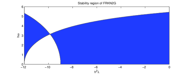
Figure 2 plots the stability region of the FRKN2G method in the $z$ and $\nu=\omega h$ plane. From Figure 2 we can see that the stability region of FRKN2G increases as $\nu=\omega h$ increases from $0$ to $\pi$, and contains the interval $[-9,0]$ for all $\nu\in[0,\pi]$. The stability region decreases as $\nu$ increases from $\pi$ to 5.4. When $\nu$ is in the interval $[5.5,2\pi]$, FRKN2G is unstable for any small $z$, or equivalently, for any small stepsize $h$. This suggests not to use FRKN2G with $\nu\in[5.5,2\pi]$. Moreover, when using FRKN2G one should restrict $\nu$ to be in the interval $[0,\pi]$ to have large stability regions. It is known that the coefficients of FRKN methods converge to those of the corresponding classical RKN methods. Thus, the limit of the stability region of FRKN2G as $\nu$ tends to zero is the same as the stability region of RKN2G. From Figure 2 one can see that the stability region of FRKN2G is slightly larger than that of RKN2G when $\nu\in[0,\pi]$.

Figure 2. Plots of stability region (shaded) of the FRKN2G method for various value of $\nu=\omega h$.

6.2. Numerical experiments

In this section we implement the 2-stage FRKN2G method derived in section 6.1, and then compare it with the RKN2G method.

In the first experiment we solve equation (6.1) by FRKN2G and RKN2G for $e=0.5$. Table 1 shows the numerical results obtained by the two methods. It is clear from equation (6.2) that if $e$ is large, then the solution of equation (6.1) is not well approximated by a linear combination of $\cos t$ and $\sin t$. Thus, for large values of $e$, we do not expect FRKN2G to be better than RKN2G. From Table 1 one can see that RKN2G is slightly better than FRKN2G. However, the difference between the two methods is insignificant.

Table 1. Errors $\triangle y_{i}=\log_{10}\displaystyle\max_{t_{0}\leq t_{n}\leq t_{N}}|y_{i}(t_{n})-y_{i,\text{comput}}(t_{n})|$ over $N$ integration steps for the two components $i=1,2$ when $e=0.5$.

		FRKN2G		RKN2G
	$h$	$\triangle y_{1}$	$\triangle y_{2}$	$\triangle y_{1}$	$\triangle y_{2}$
	$1/2^{~{}}$	-0.1555	-0.0703	-0.0643	-0.0009
	$1/2^{2}$	-1.4358	-1.2576	-1.4889	-1.3038
	$1/2^{3}$	-3.0069	-2.7745	-3.1459	-2.8956
	$1/2^{4}$	-4.1495	-3.9321	-4.2650	-4.0354
	$1/2^{5}$	-5.3323	-5.1172	-5.4399	-5.2148
	$1/2^{6}$	-6.5308	-6.3167	-6.6365	-6.4128
	$1/2^{7}$	-7.7340	-7.5201	-7.8388	-7.6154
	$1/2^{8}$	-8.9457	-8.7315	-9.0424	-8.8192

Table 2 presents the numerical result when $e=0.01$. It follows from Table 2 that FRKN2G is much better than the classical RKN2G method. This follows from the fact that when $e$ is small the solution to equation (6.1) can be well approximated by a linear combination of $\sin t$ and $\cos t$. Indeed, in this experiment, RKN2G requires a stepsize half of the one used by FRKN2G to yield results of the same accuracy. Consequently, in this experiment, RKN2G takes twice as long as FRKN2G for the same accuracy.

Table 2. Errors $\triangle y_{i}=\log_{10}\displaystyle\max_{t_{0}\leq t_{n}\leq t_{N}}|y_{i}(t_{n})-y_{i,\text{comput}}(t_{n})|$ over $N$ integration steps for the two components $i=1,2$ when $e=0.01$.

		FRKN2G		RKN2G
	$h$	$\triangle y_{1}$	$\triangle y_{2}$	$\triangle y_{1}$	$\triangle y_{2}$
	$1/2$	-4.0500	-3.7300	-2.3942	-2.4200
	$1/2^{2}$	-5.1726	-4.8342	-3.5973	-3.5971
	$1/2^{3}$	-6.3231	-6.0228	-4.8289	-4.8213
	$1/2^{4}$	-7.5164	-7.2231	-6.0429	-6.0354
	$1/2^{5}$	-8.7176	-8.4263	-7.2502	-7.2426
	$1/2^{6}$	-9.9273	-9.6343	-8.4551	-8.4475
	$1/2^{7}$	-11.5489	-11.1156	-9.6596	-9.6519

We performed further experiments not reported here with smaller values of $e$ and observed that the smaller $e$ is, the better FRKN2G compared to RKN2G.

We also carried out experiments with a different 2-stage FRKN method constructed with coefficients found from equation (6.4) using $(c_{1},c_{2})=(0.2,1)$. This method is denoted by FRKN2 without the suffix G that was used earlier to indicate Gauss points. The corresponding 2-stage classical RKN method using $(c_{1},c_{2})=(0.2,1)$ is also simply denoted by RKN2. To improve the accuracy for computing $y^{\prime}_{n+1}$ we derived a further method using the formula

(6.5) $$y^{\prime}_{n+1}=y^{\prime}_{n}+h\tilde{d}_{0}(\nu)f(t_{n},y_{n})+h\tilde{\bm{d}}^{T}(\nu)f(\bm{e}t_{n}+\bm{c}h,\bm{Y}_{n}),$$

where the coefficients $\tilde{d}_{0}(\nu)$ and $\tilde{\bm{d}}^{T}(\nu)$ are computed so that the formula (6.5) has a local accuracy order of $s+2=4$. The resulting method with $y^{\prime}_{n+1}$ computed by (6.5) is denoted by FRKN2x. Concomitantly, we use RKN2x to denote the corresponding classical method with $y^{\prime}_{n+1}$ computed by a similar equation to (6.5).

Table 3 presents the numerical results for FRKN2, FRKN2x, RKN2, and RKN2x, for the two-body problem with $e=0.5$. It follows from the table that the accuracy orders for FRKN2 and RKN2 are both $p=2$ while the accuracy orders for FRKN2x and RKN2x are both $p=3$. This confirms our observation earlier that it is because of the accuracy order of $y^{\prime}_{n+1}$ that the accuracy of the method cannot exceed $s$ for arbitrary $\bm{c}=(c_{i})_{i=1}^{s}$. From this table one can see that the FRKN2 and FRKN2x methods are comparable to the corresponding classical RKN2 and RKN2x methods.

Table 3. Errors $\triangle y_{i}=\log_{10}\displaystyle\max_{t_{0}\leq t_{n}\leq t_{N}}|y_{i}(t_{n})-y_{i,\text{comput}}(t_{n})|$ over $N$ integration steps for the two components $i=1,2$ when $e=0.5$.

		FRKN2		FRKN2x		RKN2		RKN2x
	$h$	$\triangle y_{1}$	$\triangle y_{2}$	$\triangle y_{1}$	$\triangle y_{2}$	$\triangle y_{1}$	$\triangle y_{2}$	$\triangle y_{1}$	$\triangle y_{2}$
	$1/2^{4}$	-0.6175	-0.4361	-1.3312	-1.1528	-0.5945	-0.4147	-1.3046	-1.1290
	$1/2^{5}$	-1.2154	-1.0278	-2.2383	-2.0605	-1.1917	-1.0048	-2.2152	-2.0402
	$1/2^{6}$	-1.8149	-1.6267	-3.1432	-2.9656	-1.7909	-1.6034	-3.1217	-2.9470
	$1/2^{7}$	-2.4154	-2.2272	-4.0471	-3.8696	-2.3912	-2.2037	-4.0265	-3.8519
	$1/2^{8}$	-3.0166	-2.8284	-4.9506	-4.7732	-2.9924	-2.8049	-4.9305	-4.7559
	$1/2^{9}$	-3.6182	-3.4300	-5.8540	-5.6765	-3.5939	-3.4064	-5.8340	-5.6595
	$1/2^{10}$	-4.2201	-4.0318	-6.7573	-6.5799	-4.1957	-4.0083	-6.7373	-6.5628
	$1/2^{11}$	-4.8220	-4.6338	-7.6647	-7.4872	-4.7977	-4.6102	-7.6405	-7.4660

Table 4 presents the numerical results for the four methods FRKN2, FRKN2x, RKN2, and RKN2x when $e=0.01$. Again, it follows from Table 4 that FRKN2x and RKN2x have an accuracy order $p=3$ while the FRKN2 and RKN2 have an accuracy order $p=2$. One can see from Table 4 that the FRKN2 and FRKN2x methods are much better than the RKN2 and RKN2x methods because, as we have discussed earlier, when $e$ is small, the exact solution to the two-body problem can be well approximated by the basis $\{\cos(t),\sin(t)\}$ used to construct FRKN2 and FRKN2x.

Table 4. Errors $\triangle y_{i}=\log_{10}\displaystyle\max_{t_{0}\leq t_{n}\leq t_{N}}|y_{i}(t_{n})-y_{i,\text{comput}}(t_{n})|$ over $N$ integration steps for the two components $i=1,2$ when $e=0.01$.

		FRKN2		FRKN2x		RKN2		RKN2x
	$h$	$\triangle y_{1}$	$\triangle y_{2}$	$\triangle y_{1}$	$\triangle y_{2}$	$\triangle y_{1}$	$\triangle y_{2}$	$\triangle y_{1}$	$\triangle y_{2}$
	$1/2^{3}$	-2.7401	-2.6147	-3.8219	-3.9469	-1.7383	-1.7175	-1.7393	-1.7567
	$1/2^{4}$	-3.3446	-3.2180	-4.7298	-4.8702	-2.3078	-2.2835	-2.6401	-2.6591
	$1/2^{5}$	-3.9454	-3.8201	-5.6354	-5.7843	-2.8940	-2.8680	-3.5427	-3.5620
	$1/2^{6}$	-4.5469	-4.4222	-6.5398	-6.6932	-3.4884	-3.4614	-4.4457	-4.4649
	$1/2^{7}$	-5.1486	-5.0242	-7.4437	-7.5993	-4.0866	-4.0592	-5.3487	-5.3679
	$1/2^{8}$	-5.7505	-5.6263	-8.3477	-8.5049	-4.6868	-4.6592	-6.2517	-6.2710
	$1/2^{9}$	-6.3525	-6.2283	-9.2636	-9.4296	-5.2879	-5.2602	-7.1548	-7.1741
	$1/2^{10}$	-6.9547	-6.8305	-10.4191	-10.8514	-5.8895	-5.8617	-8.0579	-8.0772

7. Conclusion.

We studied functionally fitted Runge-Kutta-Nyström methods using the collocation framework that we previously introduced for functionally fitted Runge-Kutta methods. This study, therefore, fills a gap in the literature by unifying the framework for both families of methods. We recovered earlier results of Ozawa [7] regarding the order of accuracy and the superconvergence, and established new stability results. Numerical experiments showed that FRKN methods tuned for a particular problem could indeed perform better than general purpose methods.

References

- [1] J. P. Coleman and S.C. Duxbury, Mixed collocation methods for , J. Comput. Appl. Math., 126 (2000), 47–75.
- [2] R. D’Ambrosio, M. Ferro, B. Paternoster, Trigonometrically fitted two-step hybrid methods for special second order ordinary differential equations, Math. Comput. Simulat., 81 (2011), no. 5, 1068–1084,
- [3] J. M. Franco, Exponentially fitted explicit Runge-Kutta-Nyström methods, J. Comput. Appl. Math., 167 (2004), 1–19.
- [4] J. M. Franco and I. Gómez, Some procedures for the construction of high-order exponentially fitted Runge-Kutta-Nyström methods of explicit type, Comput. Phys. Commun., 184 (2013), 1310–1321.
- [5] N. S. Hoang, R. B. Sidje, N. H. Cong, On functionally-fitted Runge-Kutta methods, BIT Numer. Math., 46 (2006), no. 4, 861–874.
- [6] N. S. Hoang, R. B. Sidje, On the stability of functionally fitted Runge-Kutta methods, BIT Numer. Math., 48 (2008), no. 1, 61–77.
- [7] K. Ozawa, Functional fitting Runge-Kutta-Nyström method with variable coefficients, Japan J. Indust. App. Math., 19 (2002), 55–85.
- [8] B. Paternoster, Runge-Kutta(-Nyström) methods for ODEs with periodic solutions based on trigonometric polynomials, Appl. Num. Math., 28 (1998), 401–412.
- [9] P. J. van der Houwen, B. P. Sommeijer, N. H. Cong, Stability of collocation-based Runge-Kutta-Nyström methods, BIT Numer. Math., 31 (1991), no. 3, 469–481.