Near-infrared Thermal Emission Detections of a number of hot Jupiters and the Systematics of Ground-based Near-infrared Photometry**affiliation: Based on observations obtained with WIRCam, a joint project of CFHT, Taiwan, Korea, Canada, France, at the Canada-France-Hawaii Telescope (CFHT) which is operated by the National Research Council (NRC) of Canada, the Institute National des Sciences de l’Univers of the Centre National de la Recherche Scientifique of France, and the University of Hawaii.
Abstract
We present detections of the near-infrared thermal emission of three hot Jupiters and one brown-dwarf using the Wide-field Infrared Camera (WIRCam) on the Canada-France-Hawaii Telescope (CFHT). These include Ks-band secondary eclipse detections of the hot Jupiters WASP-3b and Qatar-1b and the brown dwarf KELT-1b. We also report Y-band, -band, and two new and one reanalyzed Ks-band detections of the thermal emission of the hot Jupiter WASP-12b. We present a new reduction pipeline for CFHT/WIRCam data, which is optimized for high precision photometry. We also describe novel techniques for constraining systematic errors in ground-based near-infrared photometry, so as to return reliable secondary eclipse depths and uncertainties. We discuss the noise properties of our ground-based photometry for wavelengths spanning the near-infrared (the YJHK-bands), for faint and bright-stars, and for the same object on several occasions. For the hot Jupiters WASP-3b and WASP-12b we demonstrate the repeatability of our eclipse depth measurements in the Ks-band; we therefore place stringent limits on the systematics of ground-based, near-infrared photometry, and also rule out violent weather changes in the deep, high pressure atmospheres of these two hot Jupiters at the epochs of our observations.
Subject headings:
planetary systems . techniques: photometric– eclipses – infrared: planetary systems1. Introduction
The robustness and repeatability of transit and eclipse spectroscopy of exoplanets – across a wide wavelength range, from the optical to the infrared, and with a variety of instruments and telescopes – is an issue of utmost importance to ensure that we can trust the understanding imparted from detections, or lack thereof, of exoplanet atmospheric features. As a result, the topic of the repeatability of transit and eclipse depth detections has attracted growing interest in recent years (e.g. Agol et al. 2010; Knutson et al. 2011; Hansen et al. 2014; Morello et al. 2014). For instance, Spitzer Space Telescope (Werner et al., 2004) measurements of the mid-infrared thermal emission of a number of hot Jupiters, largely with the IRAC instrument (Fazio et al., 2004), have already undergone a thorough number of analyses, reanalyses and intriguing revisions (e.g. Harrington et al. 2007; Knutson et al. 2009; Knutson et al. 2007; Charbonneau et al. 2008; Stevenson et al. 2010; Knutson et al. 2011). Hubble Space Telescope (HST)/NICMOS (Thompson et al., 1998) detections of transmission features in the atmospheres of exoplanets are in the midst of an ongoing, raging debate as to the fidelity of these claimed detections (e.g. Swain, Vasisht & Tinetti. 2008; Swain et al. 2009a; Swain et al. 2009b; Gibson et al. 2011; Mandell et al. 2011; Gibson et al. 2012; Waldmann et al. 2013; Swain et al. 2014).
To-date broadband near-infrared thermal emission measurements of hot Jupiters from the ground have generally been too few and far between to warrant thorough reanalyses, or attempts at demonstrating the repeatability of eclipse detections. There have been a handful of confirmations of the depths of ground-based, near-infrared secondary eclipse detections (Croll et al. 2011a; Zhao et al. 2012a; Croll 2011; Zhao et al. 2012b). However, troublingly, the early indications of the reliability of these detections has not been overwhelmingly positive. Reobservations of the thermal emission of TrES-3b in the Ks-band disagreed by 2 (de Mooij & Snellen, 2009; Croll et al., 2010b), while a ground-based H-band upper-limit appears to disagree with a space-based HST/Wide Field Camera 3 (WFC3) detection (Croll et al. 2010b; Ranjan et al. 2014). A suggested, possible detection of a near-infrared, feature in the transmission spectrum of GJ 1214b (Croll et al., 2011b), was refuted by other researchers (Bean et al., 2011). Two observations of the thermal emission of the hot Jupiter WASP-19b obtained with the same instrument/telescope configuration, analyzed by the same observer were only found to agree at the 2.9 level (Bean et al., 2013), and were arguably marginally discrepant from other measurements of the ground-based, near-infrared, thermal emission of this planet (Anderson et al. 2010; Gibson et al. 2010; Burton et al. 2012; Lendl et al. 2013). Finally, the obvious systematics in ground-based, near-infrared photometry have caused others to encourage caution when interpreting the eclipse depths returned via ground-based detections (de Mooij et al., 2011).
Complicating this picture, is the question of whether we would actually expect thermal emission depths to be identical from epoch to epoch in the first place. To-date multiwavelength constraints have often been obtained at different epochs, and thus the effective comparison of these measurements relies on the assumption that the thermal emission of these planets is consistent from epoch to epoch. One reason this would not be the case is if these planets have variable weather and intense storms, such as those that have been theoretically predicted by dynamical atmospheric models of hot Jupiters with simplified radiative transfer. Examples include the two-dimensional shallow water models of Langton & Laughlin (2008) and the three-dimensional Intermediate General Circulation model simulations of Menou & Rauscher (2009); the latter predict brightness temperature variations of 100 for a hot Jupiter similar to HD 209458.
One approach to constrain the temporal variability of a hot Jupiter is to detect its thermal emission in a single band at multiple epochs. This has already been performed with Spitzer in the mid-infrared; the Agol et al. (2010) study placed a stringent 1 upper limit on the temporal variability of the thermal emission of the hot Jupiter HD 189733 of 2.7% from seven eclipses in the 8.0 Spitzer/IRAC channel (corresponding to a limit on brightness temperature variations of 22 ). Knutson et al. (2011) place a 1 upper limit of 17% on the temporal variability of the thermal emission of the hot Neptune GJ 436 in the same 8.0 Spitzer/IRAC channel (corresponding to a limit on brightness temperature variations of 54 ). Mid-infrared limits are important, but it arguably makes more sense to search for temporal variability in the near-infrared. If we assume the planet radiates like a blackbody, then for a given temperature difference on the planet, the difference in the Planck function will be much greater at shorter wavelengths, than at longer wavelengths (Rauscher et al., 2008). For example, if we assume that mid- and near-infrared observations probe the same atmospheric layer, then a 100 temperature difference observed in the Menou & Rauscher (2009) model from eclipse to eclipse for a canonical HD 209458-like atmosphere will result in eclipse to eclipse variations on the order of 33% of the eclipse depth in Ks-band, compared to 11% of the eclipse depth at 8.0 . Alternatively, as the atmospheres of hot Jupiters are believed to be highly vertically stratified (Menou & Rauscher 2009, and references therein), and the YJHK-bands are water opacity windows and therefore should stare much deeper into the atmospheres of hot Jupiters than mid-infrared observations (Seager et al., 2005; Fortney et al., 2008; Burrows et al., 2008), it is possible that near-infrared observations may probe higher pressure regions that are variable, even if higher altitude layers are not. A useful analogue could be that of the atmospheres of brown dwarfs: the phase lags and lack of similarity in the phase curves observed at different wavelengths for variable brown dwarfs near the L/T transition (Biller et al., 2013) – supposedly due to different wavelength of observations penetrating to different depths in the atmosphere – could be analogous to highly irradiated hot Jupiters.
In this paper we present a through investigation of how to return robust detections and errors of secondary eclipses of exoplanets from ground-based, near-infrared photometry, despite the inherent systematics. Once accounting for these systematics, we are able to present robust new detections and one reanalyzed detection of the near-infrared thermal emission of several hot Jupiters (Qatar-1b, WASP-3b, and WASP-12b) and one brown dwarf (KELT-1b). The layout of the paper is as follows. We present our new CFHT/WIRCam observations of the secondary eclipses of hot Jupiters and a brown dwarf in Section 2. In Section 3, we describe our new pipeline to reduce observations obtained with WIRCam on CFHT in order to optimize the data for high-precision photometry. We analyze our secondary eclipse detections in Section 4, using the techniques discussed in Section 5; these techniques include how to constrain systematic errors, determine the optimal aperture size and reference star ensemble, and to return honest eclipse depths and uncertainties, despite the systematics inherent in near-infrared, photometry from the ground. In Section 6 we discuss the noise properties of our ground-based, near-infrared photometry, and how our precision varies for faint and bright-stars, for the same object in the same-band on several occasions, and for the same object in different near-infrared bands (the YJHK-bands). Lastly, in Section 7 we demonstrate the repeatability of our eclipse depth measurements in the Ks-band for two hot Jupiters; we are therefore able to place a limit on both the systematics inherent in ground-based, near-infrared photometry, and on the presence of weather, or large-scale temperature fluctuations, in the deep, high pressure atmospheres of the hot Jupiters WASP-3b and WASP-12b.
2. Observations
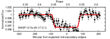
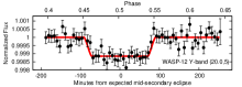
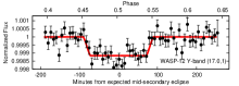
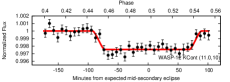
In this paper we analyze an assortment of new and previously presented ground-based, near-infrared observations of exoplanets obtained with the Wide-field Infrared Camera (WIRCam; Puget et al. 2004) on the Canada-France-Hawaii Telescope (CFHT). We discuss the new observations that we present in this paper in Section 2.1; these new observations include Ks-band eclipse detections of Qatar-1b, and the brown-dwarf KELT-1b, two Ks-band eclipse detections of WASP-3b, and a eclipse detections of WASP-12b in the Y-band, -band and two detections in the Ks-band. Other observations in this paper that have been previously discussed in other papers include our JHKs-band secondary eclipse detections of WASP-12b (Croll et al., 2011a), and our 2012 September 1 Ks-band observations of the transit of KIC 12557548b (Croll et al., 2014). We also reanalyze our Ks-band detection of the thermal emission of WASP-12b on 2009 December 28 (discussed previously in Croll et al. 2011a).
2.1. Our new CFHT/WIRCam observations of hot Jupiters and a brown dwarf
| Eclipse | Date (Hawaiian | Duration | Defocus | Exposure |
|---|---|---|---|---|
| Light curve | Standard Time) | (hours) | (mm/arc-secondsaaThe defocus value quoted in arc-seconds is the approximate radius of the maximum flux values of the defocused “donut” PSF of the target star, and is not necessarily directly proportional to the defocus value in .) | Time (sec) |
| First WASP-12 Ks-bandbbWe note that this data-set is reanalyzed here, and was presented previously in Croll et al. (2011a). | 2009 December 28 | 6.2 | 2.0/2.8 | 5.0 |
| Second WASP-12 Ks-band | 2011 January 14 | 8.5 | 1.5/2.2 | 5.0 |
| Third WASP-12 Ks-band | 2011 December 28 | 6.2 | 2.0/2.7 | 5.0 |
| WASP-12 Y-band | 2011 January 25 | 7.4 | 1.3/1.9 | 5.0 |
| WASP-12 -band | 2012 January 19 | 4.6 | 1.0/1.4 | 30.0 |
| First WASP-3 Ks-band | 2009 June 3 | 4.7 | 1.0/2.3 | 5.0/4.0 |
| Second WASP-3 Ks-band | 2009 June 14 | 5.9 | 1.5/2.4 | 3.5 |
| Qatar-1 Ks-band | 2012 July 27 | 4.0 | 1.5/2.2 | 4.5 |
| KELT-1 Ks-band | 2012 October 10 | 6.8 | 2.0/2.9 | 8.0 |
We present Ks-band (2.15 ) observations of the brown-dwarf hosting star KELT-1 (9.44), and the hot Jupiter hosting stars Qatar-1 (10.41), and WASP-3 (9.36); we also present Ks-band, Y-band (1.04 ) and -band (2.22 ) observations of the hot Jupiter hosting star WASP-12 (10.19). We observed these targets using “Staring Mode” (Croll et al., 2010a; Devost et al., 2010), where the target star is observed continuously for several hours without dithering. The observing dates and the duration of our observations are listed in Table 1. We defocused the telescope for each observation, and list the defocus value and the exposure time in Table 1. Our exposures were read-out with correlated double sampling; for each exposure the overhead was 7.8 seconds.
The conditions were photometric for each of our observations. Our 2011 December 28 observations of WASP-12b in the Ks-band suffered from poor seeing that varied from 0.8″ at the start of our observations to 2.1″ at the end. Our observations of WASP-12 in the -band on 2011 January 25 were aborted early due to a glycol leak at the telescope; as a result there is very little out-of-eclipse baseline after the secondary eclipse for that data-set. We note that for our first WASP-3 observation (2009 June 3) we used 5-second exposures for the first five minutes of the observations; for these 5-second exposures, we found that the brightest pixels in our target aperture were close to saturation, so we switched to 4-second exposures for the remainder of those observations.
3. Reduction of the “Staring Mode” WIRCam data
We have created a pipeline to reduce WIRCam “Staring Mode” (Devost et al., 2010) data, independent of the traditional WIRCam I’iwi pipeline111http://www.cfht.hawaii.edu/Instruments/Imaging/WIRCam/IiwiVersion2Doc.html. The I’iwi pipeline was originally developed to reduce all WIRCam data. Our new pipeline was developed to optimize the WIRCam data for high-cadence, photometric accuracy; each step of the I’iwi version 1.9 pipeline was investigated to determine its effect on the accuracy of the “Staring Mode” data. In Section 3.1 we discuss the details of our pipeline, and in Section 3.2 we summarize the lessons learned from the development of our pipeline that may be applicable to reduction pipelines for other near-infrared arrays, in order to optimize these pipelines for high-precision photometry.
3.1. Our Reduction Pipeline Optimized for high-precision photometry
The original I’iwi pipeline, which was applied to previous iterations of our data (Croll et al., 2010a, b, 2011a), consisted of the following steps: saturated pixel flagging, a non-linearity correction, reference pixel subtraction, dark subtraction, dome flat-fielding, bad pixel masking, and sky subtraction. Here we summarize the steps of our pipeline, and note the differences between it and the I’iwi version 1.9 pipeline:
-
•
Saturated pixel flagging: Identically to the I’iwi version 1.9 pipeline we flag all pixels with CDS values of 36,000 Analog-to-digital unit () as saturated; in a step that is not included in I’iwi, for these saturated pixels we interpolate their flux from adjacent pixels as discussed below.
-
•
The reference pixel subtraction: In contrast to the I’iwi 1.9 pipeline, we do not perform the reference pixel subtraction. In I’iwi a reference pixel subtraction was performed to account for slow bias drifts; in this step the median of the “blind” bottom and top rows of the WIRCam array were subtracted from the WIRCam array for every exposure. We observed that the reference pixel subtraction did not improve the precision of our resulting light curves; in most cases it resulted in a small increase in the root mean square (RMS) of the resulting light curves. For this reason we do not apply a reference pixel subtraction.
-
•
Bad-pixel masking: In the I’iwi pipeline a bad-pixel map is constructed that flags bad-pixels, hot-pixels and those that experience significant persistence. This method flagged a greater number of pixels as problematic than was optimal for our photometry; we discovered that a great number of the pixels flagged as “bad” were suitable for our photometry, and it was better to not flag these pixels as “bad”, than attempt to recover their flux from interpolation from nearby pixels. Therefore, we construct a bad pixel map that accepts a larger fraction of bad/poor pixels than in the normal I’iwi interpretation. Our bad pixel map is constructed from our median sky-flat (discussed below), and pixels are flagged as “bad” that deviate by more than 2% from the median of the array.
-
•
Dark Subtraction: Similarly to the I’iwi pipeline, we subtract the dark current using traditional methods. We use the standard dark frames, produced for each WIRCam run. The dark current of the WIRCam HAWAII-2RG’s (Beletic et al., 2008) is small (0.05 e-/sec/pixel), therefore this step has negligible impact on our light curves.
-
•
Non-linearity correction: We apply a non-linearity correction to our data. We utilize the WIRCam non-linearity correction using data obtained from 2007 July 16 to 2008 March 1. Extensive tests of the non-linearity correction show that for nearly all of our “Staring Mode” data-sets – those featuring relatively low sky backgrounds and modest levels of illumination – the resulting secondary eclipse depths are relatively insensitive to the non-linearity correction. However, for our Ks-band observations that feature high levels of illumination and a large sky background (such as our KELT-1 Ks-band photometry), the resulting eclipse depth depends on the non-linearity correction.
-
•
Cross-talk correction: We do not employ a cross-talk correction. The WIRCam Hawaii-2RG chips suffer from obvious artefacts due to either cross-talk, or arguably more noticeably, effects related to the 32-amplifiers on each WIRCam chip. One technique for removing these cross-talk and amplifier artefacts, is to take the median of the 32-amplifiers on each WIRCam chip for each exposure, and to subtract this median amplifier from each of the 32-amplifiers. Although this appears to remove the effects of these amplifier artefacts, it does not improve the precision (the RMS) of the resulting light curves. Therefore, we do not employ median amplifier subtraction techniques, or any other form of cross-talk correction.
-
•
Sky frame subtraction: We do not employ sky frame subtraction; we instead subtract our sky using an annulus during our aperture photometry. As our observations are continuous throughout our observations, we are unable to construct sky frames contemporaneously with our observations. Attempts to include sky frame subtraction, using the techniques discussed in Croll et al. (2010a), did not improve the RMS of the resulting photometry.
-
•
Division by a sky flat: We divide our observations by our sky-flat. We construct a sky-flat for each “Staring Mode” sequence (i.e. several hours of observing of a transit or eclipse, for instance) by taking the median of a stack of dithered in-focus images observed before and after our target observations. Usually this consists of 15 dithered in-focus observations before and after our observations. Due to the high sky and thermal background in the Ks-band, our sky-flats in that band typically have 2000 / or more, per exposure.
-
•
Interpolation over bad/saturated pixels: In the I’iwi 1.9 pipeline bad or saturated pixels were flagged with “Not-a-Number” values and therefore did not contribute to the flux in our apertures. During times of imperfect guiding, these flagged pixels would move in comparison to the centroids of our point-spread-functions (PSFs) and would occasionally fall within the aperture we use to determine the flux of our target or reference stars. When these poor pixels would fall within the aperture of our targets they would result in obvious correlated noise; when such flagged pixels fell in our reference star apertures, the effect was more subtle. To correct these discrepancies, we interpolate the flux of all bad/saturated pixels from adjoining pixels (the pixels directly above, below and to each side of the affected pixel, as long as they themselves are not bad or saturated pixels). Even still, we have noticed that our attempts at interpolating the flux of the saturated/bad pixel does not precisely capture the true flux of the pixel to the level required for precise measurements of the eclipse or transit depths of exoplanets. This is likely due in part to the fact that our defocused PSFs are not radially symmetric222This lack of radial symmetry is likely due to either astigmatism, or the effects of the secondary struts projected onto the image plane due to suboptimal telescope collimation. and display significant pixel-to-pixel flux variations, and therefore interpolation cannot precisely account for the flux of a neighbouring pixel. Due to the precision required for the science goals that we discuss here, we have found that it is preferable to throw away exposures with a saturated pixel in the aperture of our target star; the interpolation technique that we discuss here is useful for our reference stars, so in general we keep exposures with a saturated pixel in our reference star apertures (as we use the median of our reference star ensemble, in general a single discrepant point negligibly affects our resulting light cure).
3.2. Lessons for other Near-infrared Pipelines
In general, the lesson from the reduction pipeline that we describe here, optimized for precise photometry of “Staring Mode” observations (Croll et al., 2010a; Devost et al., 2010), compared to the original I’iwi pipeline, is to avoid division or subtraction by quantities that vary from exposure to exposure. The significant systematics observed in near-infrared photometry from the ground, and the large variations in flux of our target stars from one exposure to the next, mean that the accuracy we achieve is entirely dependent on our differential photometry, and the assumption that the flux of our target star closely correlates with the flux of our reference stars in each exposure. Steps, such as the reference pixel subtraction, the cross-talk correction, or the sky subtraction step, that feature subtraction or division by values that change from exposure to exposure, appear to worsen rather than improve the resulting RMS of the light curves; the likely reason is that they cause small variations, from exposure to exposure, in the ratio of the flux from the target to the reference stars. Such variations appear to lead to correlated noise in the resulting light curve.
We emphasize that generic pipelines optimized for other science goals, may therefore introduce steps that ultimately degrade the quality of the resulting photometry. One such example is the aforementioned cross-talk correction. The cross-talk step described above is crucial to remove amplifier effects that are usually visible in the processed WIRCam images; therefore this cross-talk effect is necessary for individuals performing, for instance, extragalactic work to detect low-surface brightness features around galaxies. This same cross-talk correction provides no improvement and occasionally degrades the RMS of the resulting “Staring Mode” photometry.
4. Analysis
| Eclipse | Aperture Radius | Inner Annuli | Outer Annuli | # of Stars in the | RMS of the residuals |
|---|---|---|---|---|---|
| Light curve | (pixels) | Radius (pixels) | Radius (pixels) | reference star ensemble | per exposure () |
| First WASP-12 Ks-band | 16 | 22 | 34 | 4 | 1.83 |
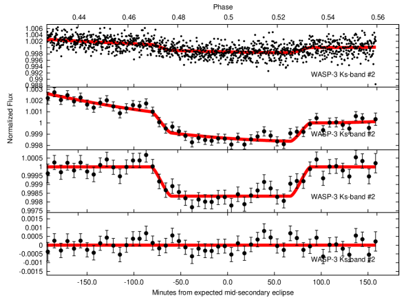
| Second WASP-12 Ks-band | 15 | 21 | 29 | 6 | 2.86 |
| Third WASP-12 Ks-band | 21 | 23 | 31 | 5 | 3.86 |
| WASP-12 Y-band | 16 | 21 | 29 | 5 | 1.59 |
| WASP-12 -band | 10 | 16 | 24 | 10 | 1.78 |
| Qatar-1 Ks-band | 14 | 19 | 28 | 5 | 1.50 |
| KELT-1 Ks-band | 19 | 22 | 30 | 4 | 1.50 |
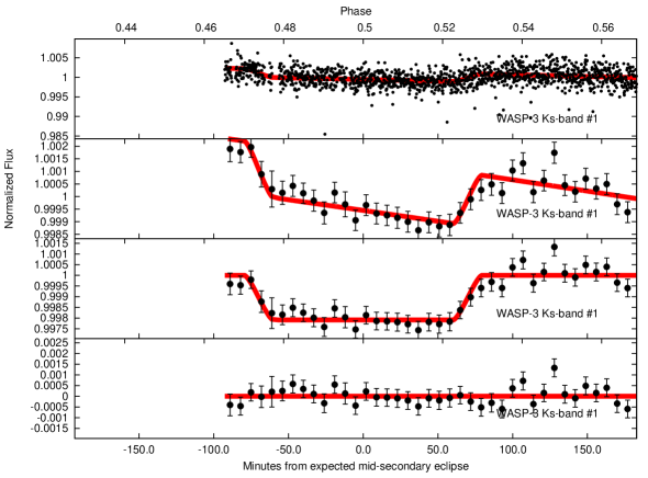
| First WASP-3 Ks-band Eclipse | 14 | 20 | 27 | 2 | 2.07 |
| Second WASP-3 Ks-band Eclipse | 16 | 20 | 29 | 1 | 1.96 |


We perform aperture photometry on our target and reference stars; we restrict our choice of reference star to those on the same WIRCam chip as the target333There are two main reasons that we restrict our choice of reference stars to the same WIRCam chip as the target; these are: (i) in previous “Staring Mode” analyses (Croll et al., 2010a, b, 2011a) we observed that the reference stars chosen were often on the same chip as the target star (it was unclear whether this was due to instrumental effects on the chip, or due to telluric affects caused by the spatial separation on the sky), and (ii) due to the extra computational time involved in running the pipeline discussed in Section 3.1, and the analysis discussed here on all four WIRCam chips, rather than just one.. We center our apertures using flux-weighted centroids. Table 2 gives the inner and outer radii of the annuli used to subtract the background for our aperture photometry. We correct the photometry of our target star with the the best ensemble of reference stars for each data-set (as discussed in Section 5.3). The reference star light curve is produced by taking the median of the light curve of all the normalized reference star light curves; each normalized reference light curve is produced by normalizing its light curve to the median flux level of that reference star. The corrected target light curve is then produced by dividing through by our normalized reference star ensemble light curve. To remove obvious outliers from our corrected target light curve, we apply a 7 cut444This outlier cut affects only our third WASP-12b Ks-band eclipse (2 points removed), our KELT-1 Ks-band eclipse (1 point removed), and our first WASP-3 Ks-band eclipse (1 point removed)..
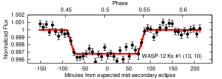
We fit our eclipse light curves with a secondary eclipse model calculated using the routines of Mandel & Agol (2002), and with a quadratic function with time to fit for what we refer to as a background trend, , defined as:
| (1) |
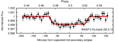
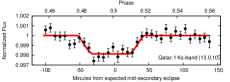
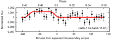
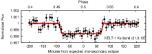
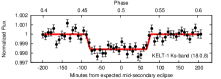
where is the interval from the beginning of the observations and , and are fit parameters. These background trends are likely instrumental, or telluric, in origin, and have been observed in several of our previous near-infrared eclipse light curves (Croll et al., 2010a, b, 2011a). The secondary eclipse parameters that we fit for are the offset from the mid-point of the eclipse, and the apparent depth of the secondary eclipse, . For WASP-12b and KELT-1b the apparent depth of the secondary eclipse is not exactly equal to the true depth of the secondary eclipse as both stars have nearby companions that dilute their depths. For our first WASP-3 secondary eclipse we do not fit for the mid-point of the eclipse, , due to the relative lack of pre-eclipse baseline, and instead assume a circular orbit (=0). We employ Markov Chain Monte Carlo (MCMC) techniques as described for our purposes in Croll (2006); we use flat a priori constraints for all parameters. We obtain our planetary and stellar parameters for WASP-3b from Pollacco et al. (2008) and Southworth (2010), for Qatar-1 from Alsubai et al. (2011), for WASP-12b from Hebb et al. (2009) and Chan et al. (2011), and for KELT-1 from Siverd et al. (2012).
To evaluate the presence of red noise in each of our photometric data-sets, we bin down the residuals following the subtraction of the best-fit model for each data-set, and compare the resulting RMS to the Gaussian noise expectation of one over the square-root of the bin size (Figure 1), for the specific aperture size and reference star ensemble given in Table 2 for each data-set. To quantify the amount of correlated noise in our data-sets we often use , a parameterization defined by Winn et al. (2008) that denotes the factor by which the residuals scale above the Gaussian noise expectation (see Figure 1). To determine we take the average of bin sizes between 10 and 80 binned points555In the odd cases where is less than one (and the data therefore scales down below the Gaussian noise limit), we set =1.. We note that most of our data-sets are relatively free of time-correlated red-noise; our second WASP-12 Ks-band eclipse, our KELT-1 Ks-band eclipse, and our first WASP-3 Ks-band eclipse, are the minor exceptions.


| Parameter | First Ks-band | Second Ks-band | Third Ks-band | Y-band | -band |
|---|---|---|---|---|---|
| Eclipse | Eclipse | Eclipse | Eclipse | Eclipse | |
| Single Aperture Size and Reference Star Ensemble Fit | |||||
| reduced | 0.913 | 1.000 | 0.739 | 0.926 | 1.159 |
| 0.00063 | 0.00100 | -0.00047 | 0.00096 | -0.00007 | |
| 0.004 | 0.003 | 0.014 | -0.002 | 0.029 | |
| 0.005 | -0.016 | -0.010 | -0.010 | -0.091 | |
| ccWe reiterate that due to the presence of the nearby M-dwarf binary companion for WASP-12, the diluted apparent eclipse depth, , is not equivalent to the true eclipse depths, , which are given in Table 5. | 0.277% | 0.286% | 0.252% | 0.100% | 0.274% |
| ()aaWe account for the increased light travel-time in the system (Loeb, 2005). | -1.5 | -2.2 | -1.2 | -0.1 | -3.0 |
| Combined Aperture Sizes and Reference Star Ensembles Fit | |||||
| ccWe reiterate that due to the presence of the nearby M-dwarf binary companion for WASP-12, the diluted apparent eclipse depth, , is not equivalent to the true eclipse depths, , which are given in Table 5. | 0.284% | 0.289% | 0.259% | 0.106% | 0.264% |
| ()aaWe account for the increased light travel-time in the system (Loeb, 2005). | -0.8 | -1.0 | -0.4 | 0.6 | -2.8 |
| bb is the barycentric Julian Date of the mid-eclipse of the secondary eclipse calculated using the terrestrial time standard (BJD-2440000; as calculated using the routines of Eastman et al. 2010). | 15194.9344 | 15576.9320 | 15924.0047 | 15587.8473 | 15946.9229 |
| 0.4995 | 0.4993 | 0.4997 | 0.5004 | 0.4982 | |
| aaWe account for the increased light travel-time in the system (Loeb, 2005). | -0.0008 | -0.0010 | -0.0004 | 0.0006 | -0.0028 |
| Parameter | Qatar-1 MCMC | WASP-3 Eclipse #1 | WASP-3 Eclipse #2 | KELT-1 MCMC |
|---|---|---|---|---|
| eclipse solution | MCMC solution | MCMC solution | eclipse solution | |
| Single Aperture Size and Reference Star Ensemble Fit | ||||
| reduced | 0.979 | 0.700 | 0.906 | 0.741 |
| -0.00005 | 0.00227 | 0.00264 | 0.00071 | |
| 0.000 | -0.012 | -0.027 | -0.001 | |
| 0.044 | -0.004 | 0.065 | -0.001 | |
| 0.121 | 0.208 | 0.164 | 0.150 | |
| ()aaWe account for the increased light travel-time in the system (Loeb, 2005). | -3.0 | 0.0ccWe do not fit for the mid-point of the eclipse, , for our first WASP-3 Ks-band eclipse. | 2.5 | -7.0 |
| Combined Aperture Sizes and Reference Star Ensembles Fit | ||||
| 0.136 | 0.234 | 0.159 | 0.160 | |
| ()aaWe account for the increased light travel-time in the system (Loeb, 2005). | -3.4 | 0.0ccWe do not fit for the mid-point of the eclipse, , for our first WASP-3 Ks-band eclipse. | 4.8 | -6.5 |
| bb is the barycentric Julian Date of the mid-eclipse of the secondary eclipse calculated using the terrestrial time standard (BJD-2440000; as calculated using the routines of Eastman et al. 2010). | 16136.8322 | 14986.9315ccWe do not fit for the mid-point of the eclipse, , for our first WASP-3 Ks-band eclipse. | 14998.0158 | 16211.8405 |
| 0.4983 | 0.5000ccWe do not fit for the mid-point of the eclipse, , for our first WASP-3 Ks-band eclipse. | 0.5018 | 0.4963 | |
| aaWe account for the increased light travel-time in the system (Loeb, 2005). | -0.0026 | 0.0000ccWe do not fit for the mid-point of the eclipse, , for our first WASP-3 Ks-band eclipse. | 0.0028 | -0.0058 |
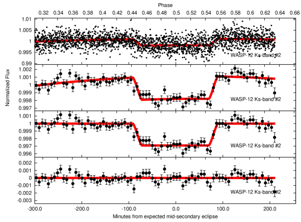
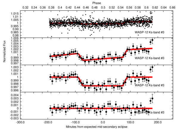
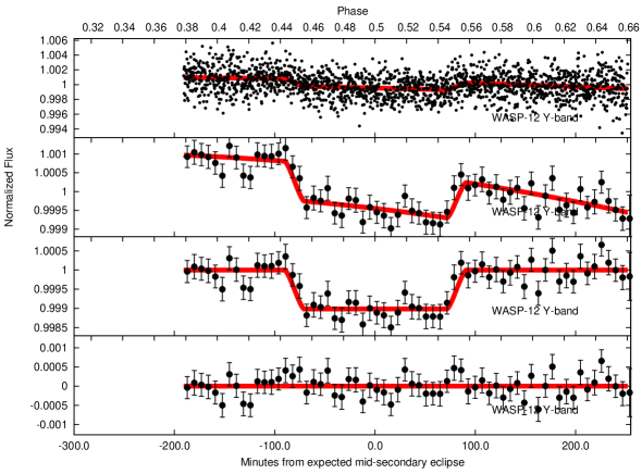
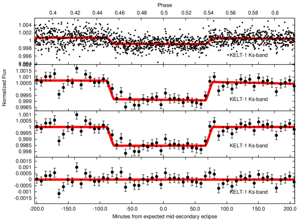
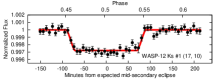
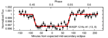
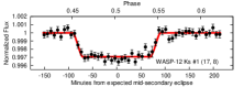
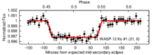
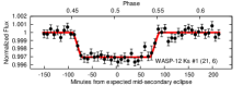
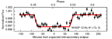
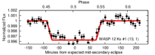
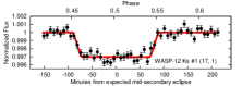
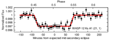
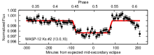
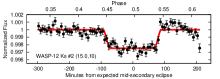
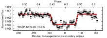
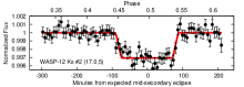
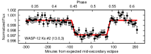
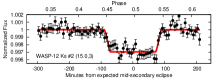
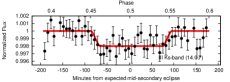
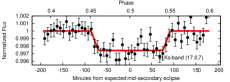
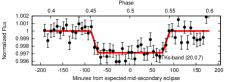
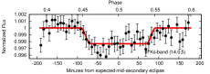
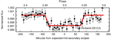
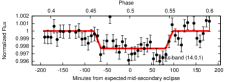
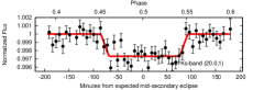
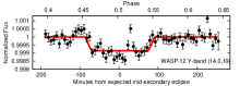
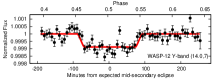
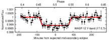
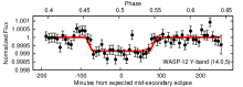
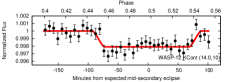
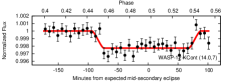
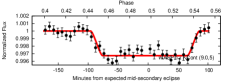
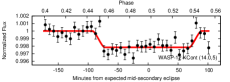
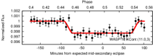
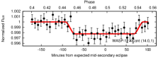
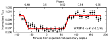
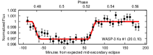
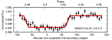
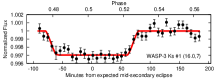
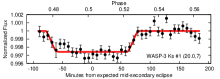
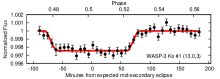
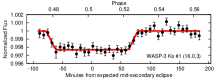
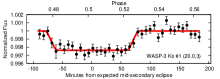
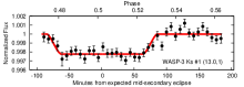
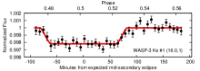
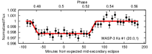
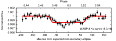
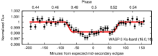
As discussed in Section 5 we extensively consider the variations in the observed eclipse depth with the size of aperture used in our aperture photometry, and the choice of reference star ensembles to correct the light curve. For reasons detailed in Section 5.1, to quantify the best-fit light curve we often use the RMS of the data following the subtraction of the best-fit light-curve multiplied by . The minimum RMS for these data-sets are found with an aperture size and number of reference stars in the reference star ensemble, as given in Table 2. It is with these aperture size and reference star ensemble choices that we present our best-fit MCMC eclipse fits for our various light curves in Figures 2 - 10. The associated best-fit parameters from our MCMC fits for a single aperture size and reference star ensemble combination are listed in the top-half of Table 3 for our WASP-12 eclipses, and at the top-half of Table 4 for our other data-sets666In Tables 3 and 4, represents the orbital phase of the mid-point of the secondary eclipses (with =0.0 denoting the transit). The associated inferred eccentricity and cosine of the argument of periastron, , of the orbit are also presented for each eclipse.. The eclipse depths and errors once we’ve taken into account the effects of different aperture sizes and reference stars, as detailed in Section 5.4, are given in the bottom of Tables 3 and 4.
4.1. Correcting the diluted eclipse depths
| Eclipse | Apparent Eclipse Depth | Actual Eclipse Depth |
|---|---|---|
| Light curve | (%) | (%) |
| First WASP-12 Ks-band | 0.284% | 0.311% |
| Second WASP-12 Ks-band | 0.289% | 0.319% |
| Third WASP-12 Ks-band | 0.259% | 0.280% |
| WASP-12 Y-band | 0.106% | 0.109% |
| WASP-12 -band | 0.264% | 0.301% |
| Qatar-1 Ks-band | n/a aaAs there are no nearby companions to dilute the secondary eclipses of these targets (or the companion is too faint as for KELT-1b; see Section 4.1), the apparent eclipse depths, , are equal to the actual eclipse depths, . | 0.136% |
| KELT-1 Ks-band | n/a aaAs there are no nearby companions to dilute the secondary eclipses of these targets (or the companion is too faint as for KELT-1b; see Section 4.1), the apparent eclipse depths, , are equal to the actual eclipse depths, . | 0.160% |
| First WASP-3 Ks-band Eclipse | n/a aaAs there are no nearby companions to dilute the secondary eclipses of these targets (or the companion is too faint as for KELT-1b; see Section 4.1), the apparent eclipse depths, , are equal to the actual eclipse depths, . | 0.234% |
| Second WASP-3 Ks-band Eclipse | n/a aaAs there are no nearby companions to dilute the secondary eclipses of these targets (or the companion is too faint as for KELT-1b; see Section 4.1), the apparent eclipse depths, , are equal to the actual eclipse depths, . | 0.159% |
| WASP-3 Ks-band combined | n/a aaAs there are no nearby companions to dilute the secondary eclipses of these targets (or the companion is too faint as for KELT-1b; see Section 4.1), the apparent eclipse depths, , are equal to the actual eclipse depths, . | 0.193 0.014% |
| WASP-12 Ks-band combined | n/a | 0.296 0.014% |
Two of our target stars, KELT-1 and WASP-12, have stellar companions that dilute their apparent eclipse depths, . Here we present our method to correct for this dilution and determine the true eclipse depths, , for these stars.
WASP-12 is in fact a triple system with an M-dwarf binary, WASP-12 BC, separated from WASP-12 by 1″, and is approximately 4 magnitudes fainter in the i-band (Bergfors et al., 2013; Crossfield et al., 2012; Bechter et al., 2014; Sing et al., 2013). This M-dwarf binary is completely enclosed within our defocused apertures. To determine the actual eclipse depths, , we correct the diluted depths, , by using the calculated factors given in Stevenson et al. (2014b) that these nearby stellar companions dilute our previous near-infrared WIRCam eclipse depths of WASP-12b (Croll et al., 2011a). These dilution factors were calculated using Kurucz stellar atmospheric models (Castelli & Kurucz, 2004) and determining the flux ratios of the models of WASP-12 to its nearby binary companion WASP-12 BC (Stevenson et al., 2014) in the JHK and z’-bands; for our Y-band, and -band secondary eclipses we simply use the Stevenson et al. (2014b) dilution factor given for the z’-band, and K-band, respectively. The actual eclipse depths, once corrected for the diluting effects of the nearby M-dwarf binary for WASP-12 using this method, are given in Table 5.
In addition to KELT-1b, KELT-1 has a nearby companion777Proper common proper motion has not been confirmed for this object, but Siverd et al. (2012) report that the likelihood of a chance alignment is minute. that is likely an M-dwarf; it is separated from KELT-1 by 0.6″ and is fainter than KELT-1 in the K-band by =5.59 magnitudes (Siverd et al., 2012). Due to the faintness of the companion compared to the target, we do not correct the secondary eclipses we report for the flux of this nearby faint companion, as the difference in the resulting eclipse depth, , is negligible.
5. Optimal techniques for ground-based, near-infrared, differential photometry
In our CFHT/WIRCam photometry of the eclipses and transits of exoplanets we have occasionally noticed that the transit/eclipse depths we measure vary by a significant amount if we choose different aperture sizes or with different reference star combinations; perhaps more troublingly, occasionally these different aperture size and reference star combinations result in very similar goodness of fits888To determine the goodness of fits we employ the RMS of the residuals multiplied by a factor to account for the correlated noise, as discussed in Section 5.1.. As the precision we are able to reach from the ground in the near-infrared relies solely on the precision of our differential photometry, it is essential that our best-fit and error-bars account for the variations due to different reference star ensembles and aperture sizes. In Section 5.1 we discuss how to choose the optimal aperture size for our ground-based, aperture photometry. In Section 5.2 we discuss the importance of taking into account the fractional contribution of pixels at the edge of the aperture in different photometry, even for large aperture sizes. In Section 5.3 we discuss how to choose the optimal reference star combination, and discuss the properties of these reference stars. Finally, in Section 5.4 we present how to return the eclipse depth and the associated error, even if there are correlations of the eclipse depth with the choice of aperture size or the choice of reference star ensemble.
5.1. Optimal Aperture Radii Choices
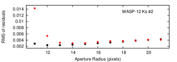


Selecting the optimal aperture radius for aperture photometry is a topic that has been receiving increasing attention by those performing high precision photometry (e.g. Gillon et al. 2007; Blecic et al. 2013; Beatty et al. 2014). In the near-infrared, where the sky background is notoriously high and contributes a large fraction of the noise budget (see Section 6), aperture size choices present a delicate balancing act between favouring small aperture sizes to minimize the impact of the high sky background, and large aperture sizes to ensure that the aperture catches all, or the overwhelming majority, of the light from the star.
In our previous analyses of the thermal emission of hot Jupiters (Croll et al., 2010a, b, 2011a), the optimal aperture choice was determined by selecting the aperture that minimized the RMS of the out-of-eclipse photometry, while clearly capturing the vast majority of the light from the star. Further investigation revealed that, due to the high sky background in the near-infrared, that if we attempted to simply minimize the RMS of the out-of-eclipse photometry, this technique, on occasion, favoured too small of aperture choices. During occasions of poor seeing or guiding, these small apertures resulted in a small amount of light near the edge of the aperture to be lost; this is apparent as time-correlated noise in many of our light-curves analyzed with small aperture (e.g. our WASP-12 Y-band photometry, or our KELT-1 Ks-band photometry; the left set of panels of Figure 16 or Figure 21).
Our preferred metric for determining the optimal aperture size, and the optimal reference star combination (see Section 5.3), is to minimize the RMS of the residuals of the photometry once the best-fit model is subtracted. We frequently observe that the minimum RMS is reached for relatively small aperture radii (for small apertures one is able to reduce the impact of the high sky background), while a lack of time-correlated noise (1) is achieved only for sufficiently large aperture values (where one is able to ensure that even during moments of poor seeing and guiding the aperture captures the vast majority of the light from the target and the reference stars); an example of the impact of aperture sizes has on eclipse depths and the precision of the light curve is displayed for our second WASP-12 Ks-band eclipse in the left panel of Figure 11. In most cases, the minimum of the RMS does a reasonable job of balancing these two competing pressures, of avoiding the high sky background that come along with large apertures, and mitigating the presence of time-correlated noise that comes along with small apertures; therefore, we select our optimal aperture choice by identifying the aperture with the minimum RMS. We note that in a previous application of this technique to near-infrared photometry (Croll et al., 2014), we used a metric of RMS; further investigation revealed that this metric did not provide a sufficiently high penalty against time-correlated noise, and occasionally resulted in light-curves with obvious time-correlated noise being favoured as the best-fit light curves.
5.2. The importance of accounting for the fractional flux at the edge of circular apertures
In this subsection, we highlight the importance for our precise, differential photometry of taking into account the fractional contribution of pixels at the edge of the circular aperture. Taking this fractional contribution of pixels into account, has become common-place in Spitzer/IRAC analyses (e.g. Agol et al. 2010), due to the fact the aperture sizes are frequently small (3-5 pixels in radius); for such small apertures, a large percentage of the pixels are near the edge of the aperture, and therefore it is imperative to take into account these edge effects.
However, the much larger apertures used in many ground-based applications, and generally in our photometry999In our previous analyses of the thermal emission and transmission spectroscopy of hot Jupiters and super-Earths (Croll et al., 2010a, b, 2011a, 2011b), aperture sizes were typically 14 - 20 pixels in radius. Our recent analysis of KIC 12557458b (Croll et al., 2014) is the exception, where we consider aperture sizes as small as 5-10 pixels; as a result, we did take into account the impact of fractional pixels at the edge of the aperture., would appear to mitigate this issue. Nonetheless, the accuracy of precise, ground-based photometry typically relies heavily on the use of differential photometry, and the assumption that the flux in a single exposure from one star is intimately associated with the flux of a reference star. Unfortunately, imperfect guiding commonly leads to small shifts in the centroid of the target and reference star PSF; this is a problem, especially for differential photometry, as the centroid of the target star may lie on one edge of a pixel, while the centroid of the reference stars may fall on different edges of their pixels. Therefore, as the target and reference star apertures shift around, the decomposition of the circular aperture into square pixels often leads to a slightly different number of pixels, and different pixels, in each aperture from one exposure to the next. In the optical, which typically features a very low sky background, this is generally not a significant problem, as apertures many times the full-width-half-maximum (FWHM) of the PSF are used and therefore at the edge of apertures there is no contribution other than the sky; however, in the near-infrared, which typically features high sky background, the lowest RMS is often achieved for apertures only fractionally larger than a few times the FWHM of the PSF (as discussed in Section 5.1), or just larger than the flux annulus for highly defocused PSFs, such as what we use in our photometry here. To mitigate this issue, we take into account the fractional contribution of the square pixels at the edge of our circular aperture, by multiplying the flux of these pixels by the fraction of the pixel that falls within our circular aperture; to do this, we utilize the GSFC Astronomy LIbrary IDL procedure pixwt.pro. We have noticed that after applying this technique our eclipse/transit depths, and our photometry, are much more robust and consistent even when varying the aperture sizes, as discussed in 5.1.
5.3. Optimal Reference Star Choices


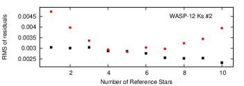
The precision of our ground-based near-infrared photometry is based solely on the accuracy imparted by our differential photometry; our 10′10′ field-of-view from a single WIRCam chip often offers 10-50 suitable reference stars. Although this is usually an asset, it can cause complications to arise if different reference star combinations, or different number of reference stars, lead to different eclipse depths, as has been observed for several of our eclipse/transit light curves (e.g. the right panels of Figure 11). As with our aperture size choices, we choose the optimal reference star ensemble by minimizing the RMS of our residuals to our best-fit light curve. In general, our experience suggests that adding additional reference stars (up to 4-10 reference stars) usually reduces the RMS, if the reference stars do not exhibit correlated noise. We therefore discuss our optimal method for choosing a reference star ensemble here.
Our most fool-proof method for choosing a reference star ensemble has been to perform and repeat our analysis – fitting for the best-fit eclipse, and background trend, as discussed in Section 4 – for reference star light curves consisting of each individual reference star. The reference star light curves with the lowest RMS are then ranked, and a reference star ensemble is composed by adding in one-by-one the best ranked (RMS) reference stars. Our full analysis is repeated until the RMS no longer improves. This process can be viewed in the right panels of Figure 11 for our second WASP-12 Ks-band eclipse.
In some cases, the use of additional reference stars does not improve the photometry. Our photometry of the second eclipse of the hot Jupiter WASP-3b is best corrected by a single reference star only, and additional reference stars only contribute correlated noise (see Figure 19). The other reference stars for our WASP-3 observation are not significantly dissimilar in colour, but are slightly fainter than the target star and the one suitable reference star (see the top-left panel of Figure 12). The reason that these other reference stars contribute significant correlated noise, may be due to an imperfect non-linearity correction.
5.3.1 Lessons for reference star selection for other programs
WIRCam (Puget et al., 2004) has an enviable 21′21′ field-of-view that many near-infrared imagers are unable to match. Even though we restrict our field-of-view in the analysis presented here to a single WIRCam chip (10′10′), we are still able to perform differential photometry on a great many more reference stars than most other infrared imagers. Our program may, therefore, be able to provide lessons for the selection of reference stars that may be applicable to others attempting to perform precise, photometry from the ground in the near-infrared.
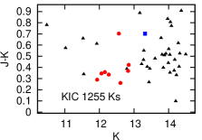
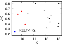
We display the magnitude and colour of our target star and the reference stars that we use to correct the flux of our target, and the reference stars that we reject for this task, for a number of our hot Jupiter light curves in Figure 12. We note that the optimal reference star ensembles appear to feature stars similar in brightness to the target star. Although these stars are often fainter than the target, this is largely due to the relative dearth of stars brighter than our typical K9-10 exoplanet host star101010There are occasionally stars brighter than our typical exoplanet host star (K9-10) on our WIRCam field-of-view, but, as we often optimize our exposure times and defocus amounts for our target, stars significantly brighter than our target often saturate, or enter into the highly non-linear regime.. KIC 12557548 is an obvious counter-example; the faintness of the target star (13.3) results in there being a wealth of reference stars brighter than the target that are useful for correcting the target’s flux. Stars significantly brighter than KIC 12557548 end up not being used in our analysis, likely due to the fact that these stars suffer from significant non-linearity, or saturate for some exposures. For our goal of high precision photometry, we note that colour of the reference stars compared to the target seems to be a secondary consideration; colour differences between the target and the reference stars do not appear to be as important as the reference stars being similar in brightness to the target star for our ground-based Ks-band photometry.
5.4. Honest Near-infrared Eclipse Depths

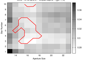


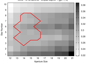


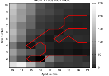


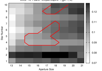


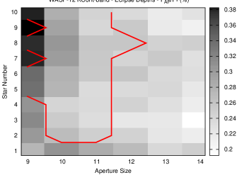


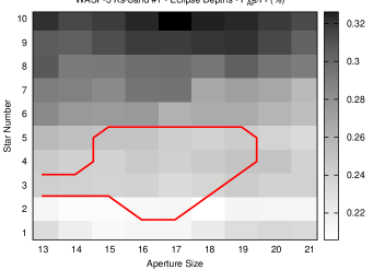


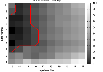
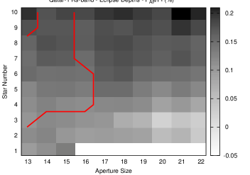


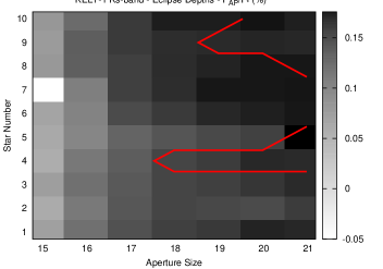


Given these occasional correlations of the apparent eclipse depth, , with the aperture size (Section 5.1) and the choice of reference star ensemble (Section 5.3), our best-fit eclipse depth and associated errors need to take into account these correlations. To do this we repeat our analysis for a variety of aperture size combinations and reference star ensembles and observe the variations in the precision (RMS) and the eclipse depths; Figure 13 displays an example of these variations for our first WASP-12 Ks-band eclipse. The same correlations with aperture size and the number of reference stars in the ensemble, are displayed for our other data-sets in Figures 14 - 21.
We consider all aperture size and reference star ensemble combinations that display nearly identical precision – that is, we consider all light curves within 15%111111Our choice of 15% above the minimum RMS was an arbitrary choice, but experience has shown it to be a reasonable compromise that captures a reasonable range of eclipse depth values for reasonably precise versions of our data-sets. For most of our data-sets the 1 error on the eclipse depth is relatively insensitive to the precise value we choose to accept above the minimum RMS. However, for data-sets that show strong variations in the eclipse depth with aperture size and the choice of reference star ensemble, such as Qatar-1 (Figure 20), the 1 error-bar on the eclipse depth does depend on the precise percentage that we accept above our minimum RMS value. of the minimum RMS observed in our grid of aperture sizes and reference star ensembles. For our first WASP-12 Ks-band eclipse, the values within 15% of the minimum RMS observed are denoted by being enclosed in the red line in the top panels of Figure 13.
To determine the accurate eclipse depth and error given these correlations with aperture size and the number of reference stars in the ensemble, we marginalize over the variations in the eclipse depths for the best RMS values (all aperture size and reference star ensembles with RMS values within 15% of the minimum RMS), by combining the MCMC chains of all these aperture size and reference star ensembles. We determine our best-fit parameters by simply applying our MCMC analysis to these combined Markov Chains. The uncertainties before and after we’ve corrected for these correlations for our various data-sets are given in Tables 3 and 4, and Figures 14 - 21.
In most, but not all cases, by employing this technique the errors on our apparent best-fit secondary eclipse depths, , marginally increase (Tables 3 and 4). The necessity of taking into account correlations of the eclipse depths with the aperture size and the number of stars in the reference star ensemble is best demonstrated by our Qatar-1 Ks-band eclipse. In Figure 20 there are a variety of reference star ensemble and aperture size combinations that fit the data with relatively similar goodness-of-fits (RMS values), that have significantly different eclipse depth values. Therefore, it is imperative that our reported eclipse depth and the associated error, take into account these correlations. The reported apparent secondary eclipse depth for our Qatar-1 Ks-band eclipse changes from = 0.121% by solely considering the single best aperture and reference star combination, to = 0.136 % by marginalizing over the various selected aperture sizes and reference star ensembles. For this reason our method should be superior to a method that just scales up the errors on by an arbitrary factor to account for systematic errors, as our method easily differentiates between those data-sets that display strong correlations with aperture size and reference star ensembles, and those that do not.
There appear to be no hard or fast rules in selecting aperture sizes and reference star combinations. Although relatively small aperture sizes are occasionally favoured (Figure 20), in other cases large apertures are favoured (Figure 21), and in others the RMS is relatively insensitive to aperture size (Figure 18). Sometimes additional reference stars only contribute correlated noise and relatively few reference stars are favoured (Figure 19), while in other cases a large number of reference stars are favoured (Figure 17).
We also repeat this analysis for the timing offset from the expected mid-point of the eclipse, . Although, we do not find strong correlations between the timing of the mid-point of our eclipses with our data-sets analyzed using our various aperture size and reference star ensembles, the different aperture size and reference star ensembles do appear to impart scatter in the timing offsets, that are greater than if they are analyzed with a single aperture size or reference star ensemble. Therefore, the true uncertainty in the mid-point of the eclipse appears to be best returned once taking into account this scatter with the various aperture size and reference star ensembles. We suspect that this method of correcting the mid-point of the eclipse for correlations with aperture size and reference star ensemble will likely limit the cases where spurious claims are made of eccentric close-in planets, due to a putative measurement of a non-zero timing offset from the expected eclipse mid-point.
6. Noise Budget of WIRCam “Staring Mode” Photometry

We also explore the noise budget of our CFHT/WIRCam “Staring Mode” photometry; the goal is to help identify the limiting systematic(s) in our ground-based, near-infrared photometry. To achieve this objective we utilize the fact that WIRCam’s large field-of-view gives us access to a great number of reference stars – ranging from bright to faint – that allow us to explore how the precision of our photometry scale with flux. We therefore perform differential photometry on each one of our 15-50 or so reference stars on the same WIRCam chip as our target star, and correct their flux with the best ensemble of these nearby reference stars, using the exact same method that we usually correct the stellar flux of our target star (except for the fact that we do not optimize our fits for each one of our reference stars for the best reference star ensemble and aperture size combination as discussed in Section 5.1 & 5.3). We correct each one of our reference stars with a four-star reference star ensemble121212The four star reference star ensemble for each “chosen” reference star are the four stars that minimize the RMS of the corrected light curve flux for each “chosen” reference star.. We use aperture sizes given in Table 2 for the WASP-3, Qatar-1, KELT-1, & new WASP-12 light curves that we discuss here; for the other light curves we use the best-fit apertures for those light curves as discussed in Croll et al. (2014) for KIC 12557548, and in Croll et al. (2011a) for the J, & H-band light curves of WASP-12b. As our reference star light curves do not (presumably) display an obvious eclipse/transit, we compute the RMS of the entire light curve; we subtract the best-fit quadratic trend from the light curve (to correct for possible systematic residual background trends as discussed in Section 4).
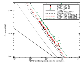
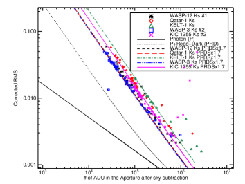
We display the resulting corrected RMS of all the reference stars of our various data-sets in Figure 22, compared to the expectation with various noise sources taken into account131313 We calculate the signal-to-noise, , of our photometry using the “CCD equation” (Merline & Howell, 1995): (2) where N is the number of ADUs from the star in the aperture, and is the gain (3.8 for WIRCam), is the number of pixels in the aperture, is the number of pixels in the annulus used to estimate the sky background, is the exposure time, is the sky noise per exposure in ADU/pixel, is the dark current (which for the WIRCam array is only 0.05 /sec/pixel, and is therefore largely negligible), is the RMS read-noise (for the WIRCam array, = /pixel/read). . As can be seen the read-noise, sky-background141414We estimate the sky background for each individual exposure by taking the median of the annulus values for each target aperture; the sky background of the light curve is then the median of these values. and photon-noise all contribute appreciably to the expected noise budget. There is an additional unknown systematic that contributes noise at approximately the same level as the sky background; as can be seen, to first-order, our data closely follows the noise limit if we multiply the sky-background by approximately 1.7 (the long-dashed line in the top panel of Figure 22, compared to the WASP-12 Ks first eclipse photometry (black stars)). The various panels of Figure 22 indicate that the sky background is one of the dominant mechanisms in determining the accuracy of our “Staring Mode” photometry; this is applicable for multiple observations of the same star in the same band (multiple observations of the star WASP-12 in the Ks-band; the top panel of Figure 22), observations of the same star in different bands (observations of WASP-12 in the YJHK and -bands; the middle panel of Figure 22), and observations of different targets in the same-band (the Ks-band; the bottom panel of Figure 22). Unfortunately, the source of the systematic that causes our light curve to scale at just less than twice the sky background level is unknown.
It is also evident that there is a subtle decrease in the expected precision for the brightest stars (the highest illumination levels, and therefore the right side of the plots in Figure 22); this is likely due to the fact that for these stars there is a lack of equally bright reference stars to correct their photometry, and that these stars often suffer from saturation or non-linearity effects.
7. Discussion
We defer the constraints that our eclipse depths provide on the atmospheres of hot Jupiters to our accompanying paper (Croll et al. in prep.). Here we present both an investigation of the timing of the mid-point of our secondary eclipses in Section 7.1, and a discussion of the repeatability of our ground-based, near-infrared eclipse depths for the hot Jupiters WASP-12b and WASP-3b in Section 7.2.
7.1. Phases of the mid-points of the transits
The mid-points of all the eclipses we present here are consistent with circular orbits, as given in Tables 3 and 4. We emphasize that one of the reasons that we find a lack of offsets from the expected mid-point of the eclipse, , is due to the fact that we have taken into account correlations of with the aperture size and reference star ensemble, as discussed in Section 5.4.
A secondary eclipse that occurs half-an-orbit after the transit, and therefore an eclipse detection that is consistent with a circular orbit, agrees with previous secondary eclipse detections for the hot Jupiter WASP-12b (Campo et al., 2011; Croll et al., 2011a; Cowan et al., 2012), and the brown-dwarf KELT-1 (Beatty et al., 2014). For WASP-3b, Zhao et al. (2012b) presented a previous detection of its thermal emission, and suggested the possibility that WASP-3b’s orbit was mildly eccentric (=0.00700.0032); our finding of = 0.0028 from our second Ks-band WASP-3 eclipse, does not support their finding of an eccentric orbit. Finally, this is the first thermal emission detection of Qatar-1b, and our secondary eclipse detection provides no evidence in favour of an eccentric orbit151515In the original Qatar-1 discovery paper (Alsubai et al., 2011) the formal radial-velocity fit slightly favoured an eccentric orbit (=0.24); however, the author’s favoured a circular orbit, and cautioned that the eccentric solution was likely spurious. A circular orbit was confirmed by Covino et al. (2013) who performed radial velocity observations of Qatar-1 and were able to place a limit on the eccentricity of the planet of: =0.020.. Our findings are consistent with the notion that whatever primordial mechanism(s) dragged these hot Jupiters, and the brown dwarf, to their present locations, if it imparted an initial orbital eccentricity, then these eccentricities have been damped away by tidal interactions with the host stars (e.g. Lin et al. 1996).
7.2. A limit on the temporal variability of two hot Jupiters
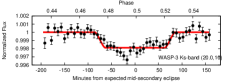
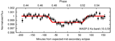
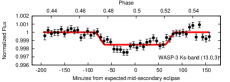
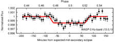
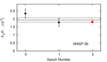
A fundamental question that has to be asked of near-infrared detections of the thermal emission of hot Jupiters from the ground is whether these eclipses are repeatable within the sub-millimagnitude errors that these depths are typically reported with (e.g. de Mooij & Snellen 2009; Croll et al. 2010a, b, 2011a; Bean et al. 2013). Another question is whether the temperatures of the deep, high-pressure layers probed by near-infrared observations (Seager et al., 2005; Fortney et al., 2008; Burrows et al., 2008) are stable, or whether they are variable due to violent storms that have been predicted by some researchers (Rauscher et al., 2007; Langton & Laughlin, 2008; Menou & Rauscher, 2009). Here we demonstrate that multiple detections of the thermal emission in the Ks-band of WASP-3b and WASP-12b largely agree with one another, and we are therefore able to place a limit on both the impact of systematic effects on ground-based, near-infrared observations, and the presence of violent storms in the deep, high pressure atmospheric layers of these two hot Jupiters. The repeatability of these eclipse depths are presented in Figure 23, and summarized in Table 5.

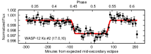
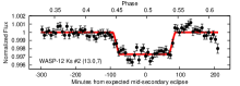
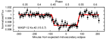
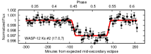
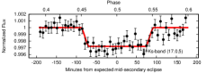
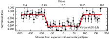
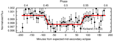
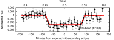
The secondary eclipse depths from our multiple detections of the thermal emission of WASP-12b in the Ks-band are displayed in the top panels of Figure 23. The weighted mean and error of our WASP-12 Ks-band observations are: = 0.296 0.014% of the stellar flux after correcting for influence of the nearby M-dwarf binary companion (Bergfors et al., 2013; Crossfield et al., 2012; Sing et al., 2013). This corresponds to a limit on the brightness temperature in the Ks-band of = 3050 . The reduced of our three WASP-12 eclipse depths are 0.3; given the size of our 1 error bars on these points, it is likely only by chance that these three eclipses are in such close agreement. Our third WASP-12 Ks-band eclipse is the most discrepant of our three eclipses, and is discrepant by less than 1. It is consistent to within 0.031% of the stellar flux of our weighted mean, or to within a temperature variation of 126.
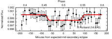
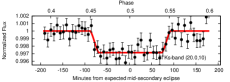
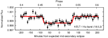
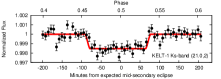
The Ks-band thermal emission of WASP-3 has already been presented in Croll (2011), and Zhao et al. (2012b). The analysis presented in Croll (2011) was a previous analysis of the data that we present here. We combine the analysis that we present here of two eclipses of WASP-3b, and the eclipse depth reported by Zhao et al. (2012b) here. The weighted mean and error of these three WASP-3 Ks-band detections are: = 0.193 0.014% of the stellar flux, corresponding to a limit on the brightness temperature in the Ks-band of = 2576 . The reduced of these three WASP-3 eclipse depths are 1.4. Our first WASP-3 Ks-band eclipse depth falls slightly outside the 1 error on our combined depth; skepticism may be warranted with our first Ks-band eclipse of WASP-3 due to the fact that it features very little out-of-eclipse baseline just prior to the eclipse. This depth is consistent to within 0.041% of the stellar flux of the weighted mean, or to within a temperature variation of 187.
The consistent eclipse depths of our WASP-12, as well as our WASP-3 eclipses, allow us to place a strict limit on the systematics inherent in ground-based near-infrared photometry. For our WASP-12 eclipses, we emphasize that the close agreement in the eclipse depths may be due to the fact that the eclipses were observed with the same telescope/instrument configuration; for the WASP-3 Ks-band eclipses the Zhao et al. (2012b) eclipse depth provides an independent confirmation with another telescope/instrument - the Palomar 5-m telescope and the WIRC instrument. Further independent measurements of the Ks-band thermal emission of WASP-3b and WASP-12b are encouraged. We note two such additional detections of WASP-12b’s thermal emission in the Ks-band have been presented by Zhao et al. (2012a); these detections feature reduced precision compared to the results we presented here, but nonetheless the weighted mean of these observations agree with our own results161616We note the important caveat that the WASP-12b eclipse depths presented in Zhao et al. (2012a) were not corrected for the dilution due to the M-dwarf binary companion to WASP-12, as these binary companions were not known at the time..
In addition to placing a limit on systematics on ground-based near-infrared photometry, our repeated eclipse depths also allow us to place a limit on epoch-to-epoch, temperature differences of the deep, high pressure region of these two hot Jupiters, due to violent storms. Menou & Rauscher (2009) predicted temperature changes on the order of 100 for a canonical HD 209458-like hot Jupiter from a three-dimensional numerical model. We are able to rule-out such large temperature variations at the epochs of two of our observations for WASP-12b, and for two of the WASP-3b observations; our first WASP-3b observation varies by 0.041% of the stellar flux (or 187) from the mean eclipse level, but the large uncertainty in the eclipse depth for our second WASP-3 Ks-band eclipse ( = 0.234%) means that there is no compelling evidence for any sort of temperature fluctuations in WASP-3b. Our limits on eclipse depth variability for the deep, high pressure regions probed by our Ks-band, near-infrared observations for the hot Jupiters WASP-12b and WASP-3b, complement previous limits in the stratospheres of the hot Jupiters using the Spitzer/IRAC instrument, including HD 189733 (Agol et al., 2010), and the hot Neptune GJ 436 (Knutson et al., 2011).
References
- Agol et al. (2010) Agol, E. et al. 2010, ApJ, 721, 1861
- Alsubai et al. (2011) Alsubai, K.A., Parley, N.R., Bramich, D.M. et al. 2011, MNRAS, 417, 709
- Anderson et al. (2010) Anderson, D.R. et al. 2010, A&A, 513, L3
- Bean et al. (2011) Bean, J.L. et al. 2011, ApJ, 743, 92
- Bean et al. (2013) Bean, J.L. et al. 2013, ApJ, 771, 108
- Beatty et al. (2014) Beatty, T.G. et al. 2014, ApJ, 783, 112
- Bechter et al. (2014) Bechter, E.B. et al. 2014, ApJ, 788, 2
- Beletic et al. (2008) Beletic, J.L. et al. 2008, in Society of Photo-Optical Instrumentation Engineers (SPIE) Conference Series, Vol. 7021, Society of Photo-Optical Instrumentation Engineers (SPIE) Conference Series
- Bergfors et al. (2013) Bergfors, C. et al. 2013, MNRAS, 428, 182
- Biller et al. (2013) Biller, B.A. et al. 2013, ApJ, 778, L10
- Blecic et al. (2013) Blecic, J. et al. 2013, ApJ, 779, 5
- Burrows et al. (2008) Burrows, A. et al. 2008, ApJ, 682, 1277
- Burton et al. (2012) Buton, J.R. et al. 2012, ApJS, 201, 36
- Campo et al. (2011) Campo, C.J. et al. 2011, ApJ, 727, 125
- Castelli & Kurucz (2004) Castelli, F. & Kurucz, R.L. 2004, arXiv:astro-ph/0405087
- Chan et al. (2011) Chan, T. et al. 2011, AJ, 141, 179
- Charbonneau et al. (2008) Charbonneau, D. et al. 2008, ApJ, 686, 1341
- Covino et al. (2013) Covino, E. et al. 2013, A&A, 554, A28
- Cowan et al. (2012) Cowan, N.B. et al. 2012, ApJ, 747, 82
- Croll (2006) Croll, B. 2006, PASP, 118, 1351
- Croll et al. (2010a) Croll, B. et al. 2010a, ApJ, 717, 1084
- Croll et al. (2010b) Croll, B. et al. 2010b, ApJ, 718, 920
- Croll et al. (2011a) Croll, B. et al. 2011, AJ, 141, 30
- Croll et al. (2011b) Croll, B. et al. 2011, ApJ, 736, 78
- Croll (2011) Croll, B. 2011, Near-Infrared Characterization of the Atmospheres of Alien Worlds, PhD thesis, Univ. Toronto (http://hdl.handle.net/1807/31726)
- Croll et al. (2014) Croll, B. et al. 2014, ApJ, 786, 100
- Crossfield et al. (2012) Crossfield, I.J.M. et al. 2012,ApJ, 760, 140
- de Mooij & Snellen (2009) de Mooij, E.J.W. & Snellen, I.A.G. 2009, A&A, 493, L35
- de Mooij et al. (2011) de Mooij, E.J.W. et al. 2011, A&A, 528, A49
- Devost et al. (2010) Devost, D. et al. 2010, Proc. SPIE, Vol. 7737, edited by David R. Silva, Alison B. Peck, B. and Thomas Soifer
- Eastman et al. (2010) Eastman, J. et al. 2010, PASP, 122, 935
- Fazio et al. (2004) Fazio, G.G. et al. 2004, ApJS, 154, 10
- Fortney et al. (2008) Fortney, J.J., et al. 2008, ApJ, 678, 1419
- Gibson et al. (2010) Gibson, N.P. et al. 2010, MNRAS, 404, L114
- Gibson et al. (2011) Gibson, N.P. et al. 2011, MNRAS, 411, 2199
- Gibson et al. (2012) Gibson, N.P. et al. 2012, MNRAS, 419, 2683
- Gillon et al. (2007) Gillon, M. et al. 2007, A&A, 466, 743
- Hansen et al. (2014) Hansen, C.J., Schwartz, J.C. & Cowan, N.B. 2014, ApJ, submitted, arXiv:astro-ph/1402.6699
- Harrington et al. (2007) Harrington, J. et al. 2007, Nature, 447, 691
- Hebb et al. (2009) Hebb, L. et al. ApJ, 2009, 693, 1920
- Knutson et al. (2007) Knutson, H. et al. 2007b, Nature, 447, 183
- Knutson et al. (2009) Knutson, H.A. et al. 2009, ApJ, 703, 769
- Knutson et al. (2011) Knutson, H.A. et al. 2011, ApJ, 735, 27
- Langton & Laughlin (2008) Langton, J. & Laughlin, G. 2008, arXiv:astro-ph/0808.3118
- Lendl et al. (2013) Lendl, M. et al. 2013, A&A, 552, A2
- Lin et al. (1996) Lin, D. N. C., Bodenheimer, P., Richardson, D. C. 1996, Nature, 380, 606
- Loeb (2005) Loeb, A. 2005, ApJ, 623, L45
- Mandel & Agol (2002) Mandel, K., & Agol, E. 2002, ApJ, 580, L171
- Mandell et al. (2011) Mandell, A.M. et al. 2011, ApJ, 728, 18
- Menou & Rauscher (2009) Menou, K. & Rauscher, E. 2009, ApJ, 700, 887
- Merline & Howell (1995) Merline, W.J. & Howell, S.B. 1995, Experimental Astronomy, Volume 6, 163
- Morello et al. (2014) Morello, G. et al. 2014, arXiv:astro-ph/1403.2874
- Pollacco et al. (2008) Pollacco, D. et al. 2008, MNRAS, 385, 1576
- Puget et al. (2004) Puget, P. et al. 2004, Proc. SPIE, 5492, 978
- Ranjan et al. (2014) Ranjan, S. et al. 2014, arXiv:astro-ph/1403.1266
- Rauscher et al. (2007) Rauscher, E. et al. 2007, ApJ, 662, L115
- Rauscher et al. (2008) Rauscher, E. et al. 2008, ApJ, 681, 1646
- Seager et al. (2005) Seager, S. et al. 2005, ApJ, 632, 1122
- Sing et al. (2013) Sing, D.K. 2013, MNRAS, 436, 2956
- Siverd et al. (2012) Siverd, R. J., Beatty, T. G., Pepper, J., et al. 2012, ApJ, 761, 123
- Southworth (2010) Southworth, J. 2010, MNRAS, 408, 1689
- Stevenson et al. (2010) Stevenson, K.B. 2010, Nature, 464, 1161
- Stevenson et al. (2014) Stevenson, K.B. 2014, AJ, 147, 161
- Stevenson et al. (2014b) Stevenson, K.B. 2014, ApJ, 791, 36
- Swain, Vasisht & Tinetti. (2008) Swain, M.R., Vasisht, G., & Tinetti, G. 2008, Nature, 452, 329
- Swain et al. (2009a) Swain, M.R. et al. 2009a, ApJ, 690, L114
- Swain et al. (2009b) Swain, M.R. et al. 2009b, ApJ, 704, 1616
- Swain et al. (2014) Swain, M.R., Line, M., & Deroo, P. 2014, ApJ, 784, 133
- Thompson et al. (1998) Thompson, R.I., M. Rieke, G. Schneider, D.C. Hines, & M.R. Corbin, 1998, ApJ, 492, L95
- Waldmann et al. (2013) Waldmann, I.P. et al. 2013, ApJ, 766, 7
- Werner et al. (2004) Werner, M.W. et al. 2004, ApJS, 154, 1
- Winn et al. (2008) Winn, J. N et al. 2008, ApJ, 683, 1076
- Zhao et al. (2012a) Zhao, M. et al. 2012a, ApJ, 744, 122
- Zhao et al. (2012b) Zhao, M. et al. 2012b, ApJ, 748, L8