The puzzling early detection of low velocity ⁵⁶Ni decay lines in SN 2014J: Hints of a compact remnant

Abstract

We show that the low-velocity ⁵⁶Ni decay lines detected earlier than expected in the type Ia SN 2014J find an explanation in the Quark-Nova Ia model which involves the thermonuclear explosion of a tidally disrupted sub-Chandrasekhar White Dwarf in a tight Neutron-Star-White-Dwarf binary system. The explosion is triggered by impact from the Quark-Nova ejecta on the WD material; the Quark-Nova is the explosive transition of the Neutron star to a Quark star triggered by accretion from a CO torus (the circularized WD material). The presence of a compact remnant (the Quark Star) provides: (i) an additional energy source (spin-down power) which allows us to fit the observed light-curve including the steep early rise; (ii) a central gravitational potential which slows down some of the ⁵⁶Ni produced to velocities of a few $10^{3}$ km s^-1. In our model, the ⁵⁶Ni decay lines become optically visible at $\sim 20$ days from explosion time in agreement with observations. We list predictions that can provide important tests for our model.

1. Introduction

SN 2014J was discovered on Jan 21 2014 (Fossey et al. 2014) in M82 at 3.5 Mega-parsecs, making it one of the closest SNe-Ia observed in recent decades. Follow-up observations suggest that SN 2014J is a normal SN Ia (Goobar et al. 2014; Ayani 2014; Cao et al. 2014; Itoh et al. 2014) and seems consistent with a delayed-detonation explosion model (Marion et al. 2014). Pre-explosion optical images of SN 2014J find no evidence for red supergiant companion stars (Goobar et al. 2014; Kelly et al. 2014), while non-detections in pre-explosion X-ray images seem inconsistent with the progenitor system being in a super-soft state just before explosion (Maksym et al. 2014; Nielsen et al. 2014). Arguments for and against the single-degenerate (SD; Whelan & Iben 1973) and the double-degenerate (DD; Iben & Tutukov 1984) scenarios have been presented in the literature (e.g. Nielsen et al. 2014; see also Diehl et al. 2014a and references therein). Churazov et al. (2014) observed SN 2014J at 50-100 days past explosion via ⁵⁶Co decay lines and derived a visible ⁵⁶Co mass of $\sim 0.2M_{\odot}$ which translates to $\sim 0.36M_{\odot}$ initial ⁵⁶Ni mass. They find a measured ⁵⁶Co expansion velocity of a few $10^{3}$ km s^-1 and argued for a standard explosion by comparing the observed line shape to their “fiducial” Chandrasekhar-mass model (their Figure 4).

A very surprising aspect of SN 2014J is the detection of 158 keV and 812 keV ⁵⁶Ni decay lines only $\sim 20$ days after the explosion (Diehl et al. 2014a). The corresponding $<2000$ km s^-1 velocities are much lower than those measured in the optical ($\sim 10^{4}$ km s^-1; Marion et al. 2014). These detections were so surprising and puzzling that Diehl et al. (2014) had to consider a model involving a Helium(He) belt with the aim of confining the resulting ⁵⁶Ni ashes to the equatorial plane. This picture might account for the low velocities of the ⁵⁶Ni decay lines if the belt is observed pole-on (their Figure 1). Besides the strong constraint on the viewing angle, there is no apparent mechanism to constrain it from spreading isotropically rather than being confined to the equatorial plane.

Here we present an alternative scenario involving a tight Neutron-Star-(CO)White-Dwarf (NS-COWD) binary where the NS experiences an explosive transition to a quark star (QS): the Quark-Nova (QN; Ouyed et al. 2002; Keränen et al. 2005; Niebergal et al. 2010). The Quark-Nova Ia (QN-Ia) is the thermonuclear explosion of the WD material following impact by the relativistic and very dense QN ejecta. A QN-Ia light curve is powered by two sources of energy: the ⁵⁶Ni decay energy and the spin-down energy from the QS. The QN-Ia has been studied in previous papers (Ouyed&Staff 2013; Ouyed et al. 2014a; Ouyed et al. 2014b; see Ouyed et al. 2011 for QNe in Low-Mass X-ray Binaries in general) where the interested reader can find details. As we argue in this paper, the QN-Ia model provides a reasonable account of the observed features of the ⁵⁶Ni decay lines in SN 2014J namely: (i) the low expansion velocities; (ii) the low optical depth at $\sim 20$ days from explosion; (iii) the amount of ⁵⁶Ni produced; (iv) the light-curve, including the early steep rise.

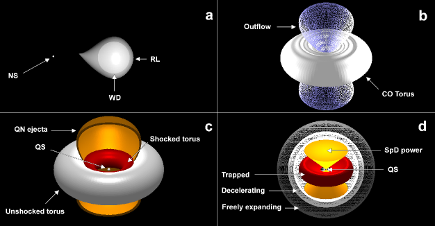
Figure 1.— Schematic diagram of QN-Ia: Panel a - A $\sim$0.6 $M_{\odot}$ WD overflows its RL and experiences unstable accretion onto a 1.7$M_{\odot}$ NS. Panel b - The WD is tidally disrupted and circularizes in a few orbital timescale around the NS forming a thick CO torus. Panel c - After accretion of $0.3M_{\odot}$ WD material, the NS experiences an explosive transition to a QS (a QN). The relativistic QN ejecta shocks and burns the torus. Panel d - After the QN shock and ejecta have left the system, some of the burnt torus material remains trapped by the gravitational potential of the QS while some of it is decelerated. The SpD power from the QS, which contributes to the QN-Ia light-curve, is illustrated as two conical lobes.

2. The Quark-Nova Ia model

In the QN-Ia, a sub-Chandrasekhar (here $M_{\rm WD,0}\sim 0.6M_{\odot}$) CO WD overflows its Roche-Lobe (RL) and accretes onto a NS via a hyper-Eddington accreting torus (Ouyed & Staff 2013; Ouyed et al. 2014a). We adopt a critical NS mass of $M_{\rm NS,c.}=2.0M_{\odot}$ at which point the QN is triggered (see Ouyed et al. 2013 for a recent review on the physics of the QN explosion). The NS mass at the end of the CE phase is taken to be $M_{\rm NS,0}=1.7M_{\odot}$ which means that for a canonical NS birth mass of 1.5$M_{\odot}$ an average of $\sim 0.2M_{\odot}$ was accreted during the CE phase (Ouyed et al. 2014a). For a typical WD mass of $0.6M_{\odot}$, it means about $0.3M_{\odot}$ needs to be accreted onto the NS to trigger the QN. The extremely dense, relativistic, QN ejecta impacts and shocks the remaining $0.3M_{\odot}$ CO torus, triggering its thermonuclear burning: the QN-Ia. In addition to the energy from the ⁵⁶Ni decay, a QN-Ia is also powered by spin-down (hereafter SpD; to be differentiated from SD which stands for Single-Degenerate) from the QS. This results in the QN-Ia obeying a Phillips-like relation where the variation in luminosity is due to SpD power (see Ouyed et al. 2014a for more details).

Figure 1 (panel a) illustrates the components in the QN-Ia model namely, an accreting NS (which eventually converts to a QS), a WD (the donor) at an orbital separation $a=a_{\rm RL}$ (the semi-major axis) which is of the order of a few $10^{9}$ cm when the WD overflows its RL (using the Eggleton (1983) formula). There are two possible outcomes once the WD overflows its RL depending on whether mass transfer is stable or unstable (e.g. Verbunt & Rappaport 1988). For mass ratio $q=M_{\rm WD,0}/M_{\rm NS,0}<\sim 0.3$ accretion proceeds in a stable manner and the WD detonates (following impact by the QN ejecta) while still in orbit at $a\sim a_{\rm RL}$ (Ouyed & Staff 2013; see also Ouyed et al. 2011). The scenario which we consider here with $q=0.35$ (panel b in Figure 1), is the unstable mass transfer regime where the WD is completely disrupted and circularizes around the NS (Fryer et al. 1999). As we show below, we do not expect any WD left when accretion onto the NS takes place. In this case, the QN-Ia results from the thermonuclear burning of the CO torus following impact by the QN ejecta (panel c in Figure 1).

2.1. Torus properties

The WD disrupts in a few orbital periods (Fryer et al. 1999) on timescales of $\sim 100$ seconds for an orbital separation of $a_{\rm RL}\sim 3\times 10^{9}$ cm. It circularizes at a radius $R_{\rm circ.}\simeq a_{\rm RL}(1+q)\left(0.5-0.227\ln{q}\right)^{4}\sim 0.4a_{\rm RL}\sim 10^{9}$ cm (e.g. Shu&Lubow 1981). The resulting thick torus (with scale-height $h_{\rm torus}\sim 0.5r_{0}$; $r_{0}$ is the torus co-ordinate) spreads outward and inward on a viscous timescale of a few $1000$ seconds for a torus with viscosity parametrized by $\alpha\sim 0.01$ (Frank et al. 1992). The characteristic accretion rate, $\sim M_{\rm WD}/t_{\rm visc.}$, is a few times $10^{-4}M_{\odot}$ s^-1.

The disrupted WD is optically thick and virializes at the circularization radius which yields a torus temperature, $T_{\rm torus}$, of the order of a few $10^{8}$ K (e.g. Paczyński 1998; assuming the torus has similar thermal and rotational energy). The torus average density ($\sim M_{\rm torus}/R_{\rm circ.}^{3}$) is of the order of a few $10^{5}$ g cm^-3. The ignition conditions for nuclear (Carbon) burning are $T_{\rm i}=5\times 10^{8}$ K and $\rho_{\rm i}=3\times 10^{6}$ g cm^-3 (e.g. Ryan & Norton 2010) so that immediately after the disruption of the WD the torus is unlikely to ignite (mainly because of the low density). The torus spreads inward and outward on a viscous timescale. If it remains virialized, the temperature increases inward as $1/r_{0}$, so the innermost part of the torus may undergo nuclear burning assuming the density increases above $\rho_{\rm i}$. Without neutrino cooling, the innermost part of the torus ($r_{0}\leq\sim 10^{8}$ cm) could undergo steady nuclear burning but it remains to be shown whether a detonation is feasible (Fernández & Metzger 2013).

3. The low-velocity ⁵⁶Ni

Once $0.3M_{\odot}$ of material has been accreted (after $\sim 1000$ seconds), the NS experiences a QN explosion. The QN ejecta and shock compresses (by a factor of a few 100) and heats (to temperatures exceeding $\sim 10^{10}$ K) the remaining $\sim 0.3M_{\odot}$ of torus material, which leads to prompt thermonuclear burning (Ouyed & Staff 2013). The expansion of the burnt torus is driven by the energy released at a velocity $v_{\rm exp.,torus}\sim 1.5\times 10^{4}\ {\rm km\ s}^{-1}$ (Arnett 1982). We assume efficient burning given the high compression and heating of the torus material: the inner parts are completely burned to ⁵⁶Ni, the central part mostly burned to ⁵⁶Ni and the outermost low-density layers are burnt to Intermediate-Mass Elements (IMEs).

For an orbit around a point mass, the velocity (from the vis-viva equation; Logsdon 1998) is $v^{2}=GM_{\rm QS}(2/r-1/a)$ which means that for a given orbit $a=$const., the velocity at a distance $r$ from the QS is

$$v(r)^{2}=v(r_{0})^{2}-v_{\rm esc.}^{2}\left(1-\frac{r_{0}}{r}\right)\ ,$$ (1)

where $v_{\rm esc.}=\sqrt{2GM_{\rm QS}/r_{0}}$ is the escape velocity at radius $r_{0}$. Here $M_{\rm QS}$ is the QS mass, and $G$ the gravitational constant. In the equation above, $v(r_{0})=v_{\rm exp.,torus}$ is the initial expansion velocity of the burnt torus (CO) material. The solid curve in Figure 2 shows the velocity at infinity ($v_{\rm\infty}$ at $r>>r_{0}$) for ⁵⁶Ni expanding from an initial radius $r_{0}$. The asymptotic velocity is reached quickly with values of $<10^{4}$ km s^-1 for $r_{0}<\sim 4500$ km while the ⁵⁶Ni ejected from higher orbits, $r_{0}$, retains a velocity close to $v_{\rm exp.,torus}$. The portion of the burnt torus at $r_{0}<r_{\rm 0,esc.}\sim 2500\ {\rm km}$ remains bound to the QS since $v_{\rm esc.}>v_{\rm exp.,torus}$ (see panel c in Figure 1 for an illustration).

The integrated mass of the torus can be derived from $M_{\rm torus}(r_{0})=\int_{r_{\rm 0,in}}^{r_{\rm 0}}2\pi\Sigma r_{0}dr_{0}$ with the surface density $\Sigma=\rho_{\rm torus}h_{\rm torus}\propto r_{0}^{-1/2}$ for $h_{\rm torus}/r_{0}=0.5$ and a torus density profile scaling as $\rho_{\rm torus}\propto r_{0}^{-3/2}$ using hydrostatic equilibrium for a gas with an adiabatic index $\gamma=5/3$. This yields $M_{\rm torus}(r_{0})/M_{\rm torus}=(r_{0}^{3/2}-r_{\rm 0,in}^{3/2})/((r_{\rm 0,out}^{3/2}-r_{\rm 0,in}^{3/2})$ where $r_{\rm 0,in}$ and $r_{\rm 0,out}$ are the torus inner and outer radii at the time of the QN explosion; $M_{\rm torus}$ is the total torus mass at the onset of the QN which is $0.3M_{\odot}$ for our fiducial values. This is shown as the dashed curve in Figure 2. About 10% of the torus material remains trapped by the QS gravitational potential, $\sim$20% decelerates to a few $10^{3}$ km s^-1 and the remainder freely expanding at speeds close to $v_{\rm exp,torus}$ (i.e. $>10^{4}$ km s^-1). The inner slowly expanding parts are very ⁵⁶Ni-rich and the outer fast moving part while mostly burned to ⁵⁶Ni, contain some IMEs in the outermost expanding layers.

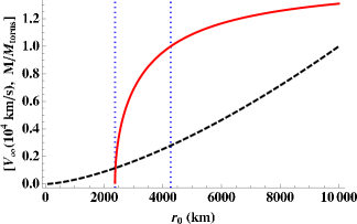
Figure 2.— The asymptotic velocity ($v_{\rm\infty}$; solid line) of the burnt torus material versus the initial radius $r_{0}$ for an initial torus expansion velocity $v_{\rm exp.,torus}=1.5\times 10^{4}$ km s^-1. The material within $r_{\rm 0,esc.}\sim 2500$ km (the left vertical dotted line) remains trapped by the QS gravitational potential. The region to the left of the second vertical dotted line (at $r_{\rm 0,esc.}\sim 4500$ km) delineates the region of strongest deceleration with $v_{\rm\infty}<10^{4}$ km s^-1. The dashed line shows the integrated torus mass $M_{\rm tours}(r_{0})$ un units of the total mass $M_{\rm torus}$.

4. The lightcurve (LC)

In addition to the energy from the ⁵⁶Ni decay, a QN-Ia is also powered by SpD energy of the newly born QS. To compute the QN-Ia LC, we use the Chatzopoulos et al. (2012) light-curve model which is a generalization of the Arnett (1980 and 1982) models. Chatzopoulos et al. (2012) provides formulae for spin-down (their eq. 13) and Nickel-decay (their eq. 9) luminosity in an homologously expanding ejecta. As explained in the Appendix here, starting with the assumptions of Chatzopoulos et al. (2012) we make additional assumptions that allow us to calculate the QN-Ia lightcurve; we also provide a link to obtain the code we used. There are essentially four physical parameters in our model namely: $M_{\rm eje.}$ (the ejected mass from the torus), $f_{\rm Ni}=M_{\rm Ni}/M_{\rm eje.}$ (⁵⁶Ni fraction of burnt torus), $P_{\rm QS}$ (the QS’s initial spin period), $B_{\rm QS}$ (the QS’s Magnetic field).

Figure 3 shows our best fit to SN 2014J data obtained by taking a QS with a period $P_{\rm QS}=18.5$ ms and $B_{\rm QS}=1.2\times 10^{15}$ G (which gives SpD timescale $\tau_{\rm SpD}\sim 11.5$ days), and a total ejecta of $M_{\rm eje.}=0.3M_{\odot}$. The amount of ⁵⁶Ni produced (up to $M_{\rm Ni}=M_{\rm eje.}$) for our fiducial values cannot account for the luminosity of SN 2014J, in particular at peak, so that for all cases the LC is also powered by SpD. Using lower Nickel fraction, $f_{\rm Ni}$, values makes the need for SpD power even more dominant. Best fits were obtained by taking the explosion date relative to the time of peak $m_{\rm B}$ to be at approximately -16.5 days. Our model is less accurate beyond $\sim$ 30 days past peak because our calculation of the photospheric radius only applies in the optically thick regime (see Appendix). The observed early steep rise of the LC is naturally captured in our model as a consequence of the SpD power injection. In our model, QNe-Ia with 5 ms $<P_{\rm QS}<$ 35 ms will display a Phillips relationship (i.e. will be accepted by the LC fitters; Figure 4 in Ouyed et al. (2014a)). Thus the $P_{\rm QS}$ suggested by our fits means that SN 2014J should obey the Phillips relationship (Phillips 1993).

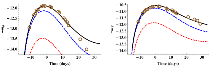
Figure 3.— Fit to apparent B-band (left panel) and V-band (right panel) SN 2014J data (Marion et al. 2014; time 0 corresponds to peak $m_{\rm B}$). The best fit (solid line) was obtained for ejected mass $M_{\rm eje.}=0.3M_{\odot}$ with a Nickel fraction of 0.75 and powered additionally by the SpD power of a $P_{\rm QS}=18.5$ ms and $B_{\rm QS}=1.2\times 10^{15}$ G QS (see Table in the Appendix). We adopt extinctions of $A_{\rm V}=1.8$ and $A_{\rm B}=3.0$ (Marion et al. 2014). The red-dotted (blue-dashed) line is the pure Nickel (pure SpD) model with $M_{\rm eje.}=0.3M_{\odot}$ powered solely by ⁵⁶Ni decay (SpD).
 

5. The optical depth in $\gamma$-rays

The column density of the spherically outer fast moving torus material ($\sim$ 70% of the total ejected mass) is estimated to be

$$\rho_{\rm col.}\sim\frac{M_{\rm fast}}{4\pi R_{\rm exp.,fast}^{2}}\sim 13\ {\rm g\ cm}^{-2}\frac{M_{\rm fast,0.2}}{v_{\rm fast,10000}^{2}t_{20}^{2}}\ ,$$ (2)

with $R_{\rm exp.,fast}=v_{\rm fast}t$; $v_{\rm fast,10000}$ is the velocity of the outer expanding torus in units of 10000 km s^-1, $t_{20}$ is time from explosion in units of 20 days and $M_{\rm fast,0.2}$ in units of $0.2M_{\odot}$.

The observed low-velocity ⁵⁶Ni decay lines are from the low-velocity material (the $\sim$ 10% decelerated part of the torus with a bulk velocity $v_{\rm slow}\sim 5000$ km s^-1). The average value of $\cos(\theta)$ over a half hemisphere is 0.5 where $\theta$ is the angle of the velocity of the expanding torus material with respect to the line-of-sight. Assuming that the Nickel lines are observed from the approaching hemisphere, $v_{\rm line}=v_{\rm slow}/2=2500$ km s^-1. Applying equation 2 to the low-velocity material ($M_{\rm low}\sim 0.1\times 0.3M_{\odot}\sim 0.03M_{\odot}$) with $v_{\rm slow}\sim 5000$ km s^-1 yields a column density of $\sim 7$ g cm^-2. The optical depth of the fast moving part of the ejected torus ($\sim$ 13 g cm^-2) is low enough that the 158 and 812 keV lines from ⁵⁶Ni decay can escape with only a few electron scatterings: $1/\kappa_{\rm es}\sim 3$ g cm^-2 where $\kappa_{\rm es}$ is the electron scattering opacity.

6. Conclusion and predictions

The QN-Ia model seems to provide ingredients that can account for the kinematics and strength of ⁵⁶Ni decay lines observed in SN 2014J (Diehl et al. 2014a). The crucial differences between our model and the standard SD and DD scenarios are:

(i) The presence of a gravitational point mass (the QS) which slows down and traps some of the burnt torus material. In the SD and DD scenarios a compact remnant may form via the Accretion-Induced-Channel channel but in that case no SN-Ia is expected or any significant amount of ⁵⁶Ni (Nomoto & Kondo 1991).

(ii) The SpD power which provides an additional energy source. One could argue for a similar scenario involving a magnetar (Duncan & Thompson 1992). For example, in the scenario which has a disrupted WD undergoing detonation (Fernández & Metzger 2012), the resulting ashes can have additional power from the magnetar’s SpD. However, there is no apparent mechanism to preserve the magnetic dipole field from the time of primary star Supernova (i.e. Magnetar formation) to the WD disruption event, tens of millions of years later. Besides providing the SpD, the QN provides a means (the QN ejecta) to compress, heat and ignite the torus.

Our model relies on the feasibility of the QN explosion. Numerical simulations of the burning of a NS to a QS with consistent treatment of reactions (including neutrinos), diffusion, and hydrodynamics find instabilities that could lead to a detonation (Niebergal et al. 2010; see also Herzog & Röpke 2011). A “core-collapse” QN could also result from the collapse of the strange quark matter core (Ouyed et al. 2013). More sophisticated high-resolution simulations are ultimately required to confirm that the QN is feasible.

6.1. Predictions

In the context of SN 2014J, among the predictions that can be tested in the near future are (see Ouyed et al. 2014b for an extended list) :

• Churazov et al. (2014) measured ⁵⁶Ni mass and velocity which are roughly in agreement with our model. Churazov et al. (2014) account for the discrepancy between the ⁵⁶Ni measured mass the $M_{\rm Ni}\sim 0.77M_{\odot}$ derived from peak luminosity by appealing to optical depth in $\gamma$-rays. We argue that the discrepancy is due to SpD energy, thus we predict that there will be no substantial increase in ⁵⁶Co in future observations. This prediction provides a crucial test of SN 2014J as a QN-Ia.

• The fast ⁵⁶Ni in Figure 2 should be seen in early ($\sim$ 20 days) spectra as broad and blue-shifted (both by $\sim$ 5%) lines. This might be testable from the early $\gamma$-ray observations of SN 2014J (e.g. Diehl et al. 2014a).

• The QS’ current spin period (6 months after explosion) is $\sim$ 40 ms. The QS is an aligned rotator (Ouyed et al. 2006) from which X-ray pulsation would be seen if there is accretion (e.g. from trapped burnt torus material).

• One could detect signatures of the Keplerian profile (double-peaked lines) from the ashes of the burnt torus material if some of it remained trapped ($\sim 0.03M_{\odot}$) by the QS gravitational potential.

• If the QS turns to a Black Hole early following the explosion, this could be observed as a “glitch” in the LC as the SpD energy is suddenly extinguished (Ouyed et al. 2014b).

Appendix A QN-Ia model LC and associated code

A.1. Model assumptions

We are using the Chatzopoulos et al. (2012) light-curve model which is a generalization of the Arnett (1980 and 1982) models. Chatzopoulos et al. (2012) provides formulae for spin-down (their eq. 13) and Nickel-decay (their eq. 9) luminosity in an homologously expanding ejecta. This means we adopt their assumptions (see Appendix A in Chatzopoulos et al. (2012) and also section II.a in Arnett 1982) which we list here:

i) Homologously expanding ejecta ($v\propto r$) and a radial density profile given by an arbitrary continuous function $\eta(r)$.

ii) Power source given by eq. A6 in in Chatzopoulos et al. (2012) with radial distribution given by a centrally concentrated function $\zeta(r)$.

iii) Radiation-pressure dominated with a temperature distribution given by $\psi(r)$ with the restriction that $\zeta(r)\eta(r)/\psi(r)$ is a constant (this assumption is required to obtain the semi-analytical solutions for the LC).

iv) The output luminosity is the diffusion luminosity as given in eq.(2) in Chatzopoulos et al. (2012).

v) The optical and $\gamma$-ray opacity is taken to be the Thompson opacity of $0.33$ cm² g^-1 corresponding to a fully ionized solar metallicity material; i.e. the composition is assumed to be fully ionized solar material for the radiative transfer problem.

In addition we add the following assumptions:

vi) We assume that the radiative transfer solution of Chatzopoulos et al. (2012) for ⁵⁶Ni luminosity is not affected by the SpD luminosity and in turn that the radiative transfer solution for the SpD luminosity is not affected by the ⁵⁶Ni luminosity. This allows us to take the QN-Ia Model total Luminosity to be additive (i.e. is given by $L_{{}^{56}Ni}+L_{\rm SpD}$). This is partly justified since in the Chatzopoulos et al. (2012) model the power input is assumed to not affect the expansion dynamics. By considering the case of equal SpD and ⁵⁶Ni luminosities, and using eq. A2 in Chatzopoulos et al. (2012), we estimate an error caused by this assumption of about 20% or less.

vii) The ejecta velocity is dominated by the burning of CO to ⁵⁶Ni which overwhelms either SpD (for $P_{\rm QS}>$ 5 ms) or ⁵⁶Ni decay energy. This gives an expansion velocity $v_{\rm exp.}\propto f_{\rm Ni}^{1/2}$ (Arnett 1982).

viii) To get an effective temperature we calculate a photospheric radius $R_{\rm ph.}$ for uniform ejecta (at fixed time) and assume a blackbody spectrum. It means our LC model is applicable only during the optically thick phase. The photospheric radius is given by : $R_{\rm ph.}=R_{0}+v_{\rm exp}t-2\lambda/3$ with $\lambda$ the photon mean-free-path. The second term includes the first-order effect of inward recession of the photosphere; e.g. Arnett 1982).

A.2. Model parameters and fitting procedure

The QN-Ia model has six free parameters: $M_{\rm eje.}$ (the ejected mass from the torus), $f_{\rm Ni}$ (⁵⁶Ni fraction of the burnt torus), $P_{\rm QS}$ (the QS’s initial spin period which affects spin-down luminosity and timescale), $B_{\rm QS}$ (the QS’s initial magnetic field which affects spin-down luminosity and timescale), $\tau_{\rm shift}$ (the model’s explosion day relative to time of peak $m_{\rm B}$), and finally $R_{0}$ (the radius at shock breakout). The $\tau_{\rm shift}$ is related to the unknown explosion date and is not related to the explosion physics. Also, because $R_{0}$ is negligible for WD explosion models we effectively have four free physical parameters.

Since the LC is spin-down dominated in our model (because of the observed low $\gamma$-ray optical depth, which means $M_{\rm eje.}\leq 0.3M_{\odot}$), $L_{\rm SpD}\propto B_{\rm QS}^{2}/P_{\rm QS}^{4}$ is approximately constant when fitting the SN2014J LC; best fits are obtained when $B_{\rm QS,15}\sim 3.5\times 10^{-3}P_{\rm QS}^{2}$, effectively reducing the number of free parameters to three. Since the SpD timescale is $\tau_{\rm SpD}\propto P_{\rm QS}^{2}/B_{\rm QS}^{2}$ this means that $\tau_{\rm SpD}\propto P_{\rm QS}^{-2}$. In other words, a shorter period would give a longer $\tau_{\rm SpD}$ which translates to a slower spin-down decay. To compensate one would need a shorter diffusion time ($\tau_{\rm d}\propto M_{\rm eje.}^{1/2}/f_{\rm Ni}^{1/4}$) thus a lower ejecta mass $M_{\rm eje.}$ or a higher $f_{\rm Ni}$; the dependency on $f_{\rm Ni}$ is weaker. Upon experimenting with the fits we find that $f_{\rm Ni}$ decreases to get the ratio of B and V magnitudes correct (which we attribute to photospheric temperature effects). Once a model is obtained one can shift the explosion date relative to the time of peak $m_{\rm B}$ by $\tau_{\rm shift}$ to overlap with data. A range of acceptable fits are shown in Table 1.

Table 1Examples of acceptable fits using $B_{\rm QS,15}=3.5\times 10^{-3}P_{\rm QS}^{2}$.

$M_{\rm eje.}(M_{\odot})$	$f_{\rm Ni}$	$P_{\rm QS}({\rm ms})$	$\tau_{\rm shift}({\rm days})$
0.30	0.75	18.5	16.5
0.25	0.65	17.5	16.5
0.20	0.55	16.5	16.5

A.3. How to obtain and use the code

The code and usage instructions are freely available at:
ftp://quarknova.ucalgary.ca/Codes/QNIa-LC-PACKAGE.zip.

References

- (1) Alford, M., Blaschke, D., Drago, A., et al. 2007, Nature, 445, 7
- (2) Arnett, W. D. 1980, ApJ, 237, 541
- (3) Arnett, W. D. 1982, ApJ, 253, 785
- (4) Ayani K., 2014, Central Bureau Electronic Telegrams, 3792, 1
- (5) Buballa, M., Dexheimer, V., Drago, A., et al. 2014, arXiv:1402.6911
- (6) Cao Y., Kasliwal M. M., McKay A., & Bradley A., 2014, The Astronomer s Telegram, 5786, 1
- (7) Chatzopoulos, E., Wheeler, J. C., & Vinko, J. 2012, ApJ, 746, 121
- (8) Churazov, E., Sunyaev, R., Isern, J., et al. 2014, Nature, 512, 406 [arXiv:1405.3332 ]
- (9) Diehl, R., Siegert, T., Hillebrandt, W., et al. 2014a, Science, 345, 1162
- (10) Diehl, R., Siegert, T., Hillebrandt, W., et al. 2014b, arXiv:1409.5477
- (11) Duncan, R. C. & Thompson, C. 1992, ApJ, 392, L9
- (12) Eggleton, P. P. 1983, ApJ, 268, 368
- (13) Fernández, R., & Metzger, B. D. 2013, ApJ, 763, 108
- (14) Fossey J., Cooke B., Pollack G., Wilde M., Wright T., 2014, Central Bureau Electronic Telegrams, 3792, 1
- (15) Frank, J., King, A. R. & Raine, D. “Accretion Power in Astrophysics, 2nd Edition, Cambridge University Press, Cambridge, 1992
- (16) Fryer, C. L., Woosley, S. E., Herant, M., & Davies, M. B. 1999, ApJ, 520, 650
- (17) Goobar, A., Johansson, J., Amanullah, R., et al. 2014, ApJ, 784, L12
- (18) Herzog, M., Röpke, F. K. 2011, Phys. Rev. D, 84, 083002
- (19) Iben, I. & Tutukov, A. V. 1984, ApJSupplements, 54, 335
- (20) Itoh R., Takaki K., Ui T., & Kawabata K. S., M. Y., 2014, Central Bureau Electronic Telegrams, 3792, 1
- (21) Iwazaki, A. 2005, Phys. Rev. D, 72, 114003
- (22) Kelly, P. L., Fox, O. D., Filippenko, A. V., et al. 2014, ApJ, 790, 3
- (23) Keränen, P., Ouyed, R., & Jaikumar, P. 2005, ApJ, 618, 485
- (24) Logsdon, T. 1998 (John Wiley & Sons)
- (25) Marion, G. H., Sand, D. J., Hsiao, E. Y., et al. 2014, arXiv:1405.3970
- (26) Maksym, W. P., Irwin, J. A., Keel, W. C., Burke, D., & Schawinski, K. 2014, The Astronomer’s Telegram, 5798, 1
- (27) Niebergal, B., Ouyed, R., & Jaikumar, P. 2010, Phys. Rev. C, 82, 062801
- (28) Nielsen, M. T. B., Gilfanov, M., Bogdán, Á., Woods, T. E., & Nelemans, G. 2014, MNRAS, 442, 3400
- (29) Nomoto, K. & Kondo, Y. 1991, ApJ, 367, L19
- (30) Nugent P. E., Sullivan M., Cenko S. B., et al., 2011, Nature, 480, 344
- (31) Ouyed, R., Dey, J., & Dey, M. 2002, A&A, 390, L39
- (32) Ouyed, R., Niebergal, B., Dobler, W., & Leahy, D. 2006, ApJ, 653, 558
- (33) Ouyed, R., Staff, J., & Jaikumar, P. 2011, ApJ, 729, 60
-
(34)
Ouyed, R., Niebergal, B., & Jaikumar, P. 2013, “Explosive Combustion of a Neutron Star into a Quark Star: the non-premixed
scenario” in Proceedings of the Compact Stars in the QCD Phase Diagram III (CSQCD III) conference, December 12-15, 2012, Guaruja, Brazil. Eds. L. Paulucci, J. E. Horvath, M. Chiapparini, and R. Negreiros,
http://www.slac.stanford.edu/econf/C121212/ [arXiv:1304.8048] - (35) Ouyed, R., & Staff, J. 2013, Research in Astronomy and Astrophysics, 13, 435
- (36) Ouyed, R., Koning, N., Leahy, D., Staff, J. E., & Cassidy, D. T. 2014a, Research in Astronomy and Astrophysics, 14, 497
- (37) Ouyed, R., Koning, N., Leahy, D., & Staff, J. E. 2014b, arXiv:1402.2717
- (38) Paczyński, B.1998, Acta Astronomica 48, 667
- (39) Phillips, M. M. 1993, ApJ, 413, L105
- (40) Ryan, S. G. & Norton, A. J., 2010, Stellar Evolution and Nucleosynthesis (Cambridge University Press)
- (41) Shu, F. H. & Lubow, S. H. 1981 Annual Review of Astronomy and Astrophysics, 19, 277
- (42) Verbunt, F., & Rappaport, S. 1988, ApJ, 332, 193
- (43) Whelan, J. & Iben, I. J. 1973, ApJ, 186, 1007