Predicting Lyman $\alpha$ and Mg II Fluxes from K and M Dwarfs Using GALEX Ultraviolet Photometry

Abstract

A star’s UV emission can greatly affect the atmospheric chemistry and physical properties of closely orbiting planets with the potential for severe mass loss. In particular, the Lyman $\alpha$ emission line at 1216Å, which dominates the far-ultraviolet spectrum, is a major source of photodissociation of important atmospheric molecules such as water and methane. The intrinsic flux of Lyman $\alpha$, however, cannot be directly measured due to the absorption of neutral hydrogen in the interstellar medium and contamination by geocoronal emission. To date, reconstruction of the intrinsic Lyman $\alpha$ line based on Hubble Space Telescope spectra has been accomplished for 46 FGKM nearby stars, 28 of which have also been observed by the Galaxy Evolution Explorer (GALEX). Our investigation provides a correlation between published intrinsic Lyman $\alpha$  and GALEX far- and near-ultraviolet chromospheric fluxes for K and M stars. The negative correlations between the ratio of the Lyman $\alpha$ to the GALEX fluxes reveal how the relative strength of Lyman $\alpha$ compared to the broadband fluxes weakens as the FUV and NUV excess flux increase. We also correlate GALEX fluxes with the strong near-ultraviolet Mg II h+k spectral emission lines formed at lower chromospheric temperatures than Lyman $\alpha$. The reported correlations provide estimates of intrinsic Lyman $\alpha$ and Mg II fluxes for the thousands of K and M stars in the archived GALEX all-sky surveys. These will constrain new stellar upper-atmosphere models for cool stars and provide realistic inputs to models describing exoplanetary photochemistry and atmospheric evolution in the absence of ultraviolet spectroscopy.

1 Introduction

Radial velocity, transit, and imaging methods have enabled the discovery of a variety of exoplanets ranging from hot super Earths to cold Jupiters, including confirmed terrestrial exoplanets within the habitable zone (HZ; Kasting et al. 1993) around low-mass stars. For giant and terrestrial planets alike, incident stellar emission at short wavelengths ($\lambda<$ 3000Å) affects the chemistry and evolution of an exoplanet’s atmosphere. In particular, it is the high energy of the far-ultraviolet (FUV) radiation that controls the processes of molecular photodissociation and photoionization in the planetary atmosphere (Hu et al. 2012), breaking apart important molecules such as water, methane and carbon dioxide, and potentially leading to significant mass loss. The possibility of complete evaporation of the planet atmosphere due to high UV (and corresponding particle) flux may explain the high fraction of hot dense planets around cool stars in the current exoplanet population (e.g. Wu & Lithwick 2013; Lammer et al. 2007). In the case of HZ planets, the incident UV stellar flux may also destroy biosignatures with which we hope to detect life, and/or produce false-positive biosignatures in the form of abiotic oxygen and ozone (Tian et al., 2014).

Much of the stellar UV flux is emitted from the upper-atmospheres of FGKM stars, namely the chromosphere, transition region and corona, and measurements at these short wavelengths require space-borne observatories and stars that are bright and not too distant from Earth. The FUV spectrum is dominated by Lyman $\alpha$, the resonance line of hydrogen at 1216 Å, which is emitted from the upper-chromosphere and lower-transition region temperatures of roughly 8000 to 30000 K (Fontenla et al., 1988). Linsky et al. (2013) recently highlighted the potential importance of the Lyman $\alpha$ emission line to the atmospheres of close-in planets. For example, the Sun’s Lyman $\alpha$  contributes $\sim$20% of the total flux between 1 to 1700 Å (Ribas et al., 2005), and is shown to be responsible for more than 50% of the photodissociation rate of the Earth’s H₂O and CH₄. Lyman $\alpha$’s fractional flux increases for cooler stars as the photospheric contribution decreases (Fig. 1, right) and can reach up to $\sim$70% of the total FUV flux for late M dwarfs (France et al., 2013).

In addition to the observational difficulties, predicting stellar UV flux from low-mass stars is also challenging since current models were not designed to calculate emission from the low-density regions of stellar upper-atmospheres. As a result, the UV flux received by an exoplanet is often underestimated in photochemical models (Kopparapu et al., 2012; Miguel & Kaltenegger, 2014; Tian et al., 2014). Recently, Miguel et al. (2014) demonstrated the significant impact of a star’s Lyman $\alpha$ on the photochemistry of the atmospheres of mini-Neptunes at low pressures using the GJ 436 planetary system, one of the few M dwarfs for which Lyman $\alpha$ data exist (France et al., 2013).

The total Lyman $\alpha$ emission is impossible to measure directly from stars due to scattering of the majority of the photons by the neutral hydrogen of the interstellar medium. Even for the nearest stars it is difficult to directly determine the Lyman $\alpha$ flux without using reconstruction techniques applied to high-resolution spectra currently available only with the Hubble Space Telescope’s (HST) Space Telescope Imaging Spectrograph (STIS) and Cosmic Origins Spectrograph (COS). Complicating the measurement further, one also has to take into account Earth’s own geocoronal Lyman $\alpha$ emission.

Using reconstructions from Wood et al. (2005) and France et al. (2012, 2013), Linsky et al. (2013) produced correlations of Lyman $\alpha$ line fluxes from a sample 46 FGKM stars with other spectral emission lines formed in the chromosphere, which were also observed with either STIS or COS. Although the Mg II h+k emission lines at 2802.7 and 2795.5 Å also required a correction for interstellar absorption at their cores (Wood et al., 2005; Linsky et al., 2013), they provided the most promising results possibly due to being least affected by metallicity differences. Even with large uncertainties in the Lyman $\alpha$ reconstructed fluxes, $\approx$20% for the FGK stars (Wood et al., 2005) and $\approx$30% for the M stars (France et al., 2012, 2013), the search for correlations between different activity diagnostics and Lyman $\alpha$ is extremely valuable when no other UV spectral data are available.

In view of the severe challenges of measuring or predicting Lyman $\alpha$ and Mg II for many stars, we used The Galaxy Evolution Explorer’s (GALEX) all-sky photometric surveys to search for correlations between FUV and NUV photometry and the intrinsic Lyman $\alpha$ and Mg II fluxes compiled by Linsky et al. (2013). In the absence of UV spectroscopy, such correlations will allow for estimates of the intrinsic Lyman $\alpha$ fluxes from thousands of stars within a few hundred parsecs in the GALEX archive with which to study stellar activity, provide empirical constraints for new cool-star upper-atmosphere models (S. Peacock et al., in preparation) and estimate the incident high-energy radiation affecting the photochemisty and evolution of planetary atmospheres.

2 GALEX NUV and FUV Photometry

The GALEX satellite was launched on 2003 April 28 and observed the UV sky until its mission completion on 2013 June 28. GALEX imaged approximately 3/4 of the sky simultaneously in two UV bands: FUV 1350–1750 Å and NUV 1750–2750 Å, excluding the powerful and complicated Lyman $\alpha$ and nominally sensitive to the Mg II h+k chromospheric lines. The average FWHM of the PSFs are 6.5″ and 5″ in the FUV and NUV, respectively, across a 1.25^∘ field of view. The full description of the instrumental performance is presented by Morrissey et al. (2005). With the failure of the FUV detector in 2009 May, subsequent observations only provided NUV imaging. The fluxes and magnitudes averaged over the entire exposure were produced by the standard GALEX Data Analysis Pipeline (ver. 4.0) operated at the Caltech Science Operations Center (Morrissey et al., 2007). The current database contains 214,449,551 source measurements (Bianchi 2013) recorded by the All-sky, Medium and Deep Imaging Surveys and many guest investigator programs. The data products are archived at the Barbara A. Mikulski Archive for Space Telescopes (MAST).

For this study we used the “aper_7” aperture for the UV photometry, which has a radius of 17.3″. This large aperture requires the least aperture correction (0.04 mags in both the in NUV and FUV bandpasses) and accounts for all possible point spread functions, even those elongated near the edges of the images. We excluded detections beyond 0.59^∘ from the center of the image to avoid the worst edge effects.

For F and G stars, the flux in the GALEX bandpasses includes a significant fraction of continuum (i.e. photospheric) emission (Fig. 1, right; Smith & Redenbaugh 2010) with the remaining flux provided by strong emission lines (C IV, C II, Si IV, He II) originating from the stellar upper-atmosphere. K and M stars have FUV and NUV fluxes strongly dominated by these stellar emission lines making GALEX an excellent tool with which to study stellar activity in lower-mass stars (e.g. Robinson et al. 2005; Welsh et al. 2006; Pagano 2009; Findeisen & Hillenbrand 2010; Shkolnik et al. 2011; Rodriguez et al. 2011; Shkolnik 2013).

Twenty-eight of the stars with reconstructed Lyman $\alpha$ fluxes compiled by Linsky et al. (2013) were observed by GALEX. These are summarized in Table 1. GALEX observations move into the non-linear regime after 34 counts s^-1 in the FUV and 108 counts s^-1 in the NUV (Morrissey et al., 2007). This required us to omit all the bright stars with effective temperatures $T_{\rm eff}$ $>$ 4900 K from the NUV analysis and one nearby K star from the FUV analysis. One M star has an FUV flux below the detection threshold and we calculate its 1-sigma upper limit using Figure 4 of Shkolnik & Barman (2014). This left eight stars with NUV detections and nineteen stars with FUV detections for analysis.

3 Analysis

Linsky et al. (2013) compiled the spectral types (SpTs), distances, and reconstructed Lyman $\alpha$ and Mg II fluxes scaled to 1 AU of 46 stars. Table 1 lists the 28 of these stars observed by GALEX. We scaled the fluxes to the stellar surface using radii derived from the Baraffe et al. (1998) models with published stellar ages from the literature and $T_{\rm eff}$ from Kraus & Hillenbrand (2007) for the given SpT.

As mentioned above, the GALEX bandpasses consist of both photospheric and chromospheric emission. We determined photospheric emission from stellar atmosphere models, which by design exclude chromospheric emission, to isolate the excess flux originating solely from upper-atmospheric activity. We adopt the semi-empirical results from Findeisen et al. (2011) who calculated GALEX FUV and NUV magnitudes of the photospheric fluxes for B8 to K5 stars using the solar-metallicity Kurucz models and applied $T_{\rm eff}$ corrections to fit empirical color-color plots. (See their Table 1 and Figure 5.) For stars cooler than K5, we use the Phoenix model atmospheres (Hauschildt et al. 1997; Short & Hauschildt 2005) convolved with the relevant NUV and FUV normalized transmission curves. (See Section 3 of Shkolnik & Barman 2014). Fig. 1 (left) plots the surface photospheric flux for our sample as a function of $T_{\rm eff}$: the Findeisen et al. (2011) fluxes for stars hotter than 4000 K and Phoenix model fluxes for cooler stars. The tight correlation between the two photospheric flux sources demonstrates their consistency.

In both the NUV and FUV detections of our sample, 80% of the targets have photospheric contributions of $<$10% of the observed flux. Only one hot star at $T_{\rm eff}$=6800 K appears to have nearly no chromospheric emission. Fig. 1 (right) plots the ratio of photospheric flux to the observed FUV and NUV surface fluxes as a function of $T_{\rm eff}$ for our sample. All but one of the K and M stars have negligible photospheric contributions. The observed and excess NUV and FUV fluxes for the sample are listed in Table 1. Although in most cases the expected photospheric flux is relatively low, we subtract it from the GALEX observations such that correlations can be made using only upper-atmospheric emission with the Lyman $\alpha$ and Mg II chromospheric line (Fig. 2). Within uncertainties, correlations for the K and M stars are unchanged by this step. (See Table 2.)

We separated the stars into two SpT bins: F and G stars and K and M stars for several reasons: (1) The fraction of the photosphere in the hotter stars is much higher than in the cooler stars for which it is effectively negligible. Thus, any uncertainties in the models used will not disrupt the results for the K and M stars, as it might for the hotter stars. (2) Low mass stars tend to have higher flare activity levels, so the non-contemporaneous data sets used in this study may induce added scatter for K and M stars. (3) And, with K and M stars being the most favorable for followup studies of HZ planets (e.g. Tarter et al. 2007; Scalo et al. 2007; Heller & Armstrong 2014), a separate correlation for these stars is appropriate for providing Lyman $\alpha$ and Mg II flux estimates with which to study planetary atmospheres.

Fig. 2 (left) shows the FUV excess to Lyman $\alpha$ surface flux correlation for the 11 K and M stars with a correlation coefficient $R$=0.91, excluding the one upper limit. The F and G correlation has eight stars with a weaker correlation coefficient R=0.63 and low statistical significance. Fig. 2 (right) shows the correlation for the Lyman $\alpha$ surface flux against the NUV excess surface flux with a strong correlation of $R$=0.94 for eight K and M stars. Due to the brightness of the F and G stars, no NUV observations were reliable due to the non-linearity of the GALEX data.

Linsky et al. (2013) pointed out that of all the emission lines they studied, Mg II may provide the most accurate Lyman $\alpha$ predictions as metallicity effects appear the smallest. Our analysis also exhibits highly significant correlations between GALEX fluxes and the Mg II lines for the K and M stars (Fig. 2, bottom). Fig. 3 shows the ratio of Lyman $\alpha$ to the GALEX flux as a function of FUV and NUV flux. These correlations reveal how the relative strength of the Lyman $\alpha$ compared to the broadband fluxes weakens as the FUV and NUV excess flux increases. All of the regression fits to the correlations are summarized in Table 2.

4 Summary

Lyman $\alpha$ is the strongest stellar UV emission line and provides the most important source of radiative losses in a star’s upper-chromosphere and lower-transition region. As such, it may also be the greatest source of molecular photodissociation in the atmosphere of an orbiting exoplanet. Measuring a star’s intrinsic Lyman $\alpha$ flux requires space-based high-resolution FUV spectroscopy plus intricate reconstruction techniques to correct for interstellar absorption and geocoronal emission. In order to gain access to the Lyman $\alpha$ emission of many more stars than is currently possible to observe (i.e. with HST), we sought to find correlations between literature values of reconstructed Lyman $\alpha$ emission and broadband stellar upper-atmospheric emission measured from GALEX FUV and NUV photometry.

Our sample consisted of the 28 stars which have both reconstructed Lyman $\alpha$ and GALEX observations ranging in SpT from F5 to M5.5. We separated our sample into 11 F and G stars and 17 K and M stars as the photospheric contribution to the GALEX bandpasses, stellar variability, and chromospheric temperature structure (e.g. Walkowicz & Hawley 2009) differ in the two groups. The F and G stars were limited to only eight FUV observations as they were too bright for reliable NUV measurements. There is a weak correlation between the FUV excess flux and Lyman $\alpha$, and a strong one between GALEX/FUV and the Mg II doublet, the strongest emission feature in the NUV spectral region. However, with the few data points for F and G stars, their small flux distribution, and uncertainties in the model fluxes, these correlations should be applied cautiously.

For the sample of K and M stars where the photospheric model fluxes are negligible, we find that the Lyman $\alpha$ surface fluxes correlate well with both the FUV and NUV excess surface fluxes such that log [$F_{Ly\alpha}$] = (0.43 $\pm$ 0.07) * log [$F_{FUV,exc}$] + (3.97 $\pm$ 0.36) and log [$F_{Ly\alpha}$] = (0.45 $\pm$ 0.07) * log [$F_{NUV,exc}$] + (3.55 $\pm$ 0.41). For stars too bright in the NUV, the FUV correlation can be used, and for more distant stars where the FUV is not detected, the NUV correlation can be used. Additionally, the GALEX excess fluxes for K and M stars correlate well with the Mg II lines providing another window into a strong stellar chromospheric emission feature probing lower emission temperatures.

With good correlations in both GALEX bandpasses, estimates of intrinsic Lyman $\alpha$ and Mg II can now be made for thousands of K and M stars out to a few hundred parsecs from Earth. These data will constrain a new and much-needed suite of model chromospheres, as well as provide planetary atmosphere models with more realistic Lyman $\alpha$ and Mg II values without the need for high-resolution UV spectroscopy.

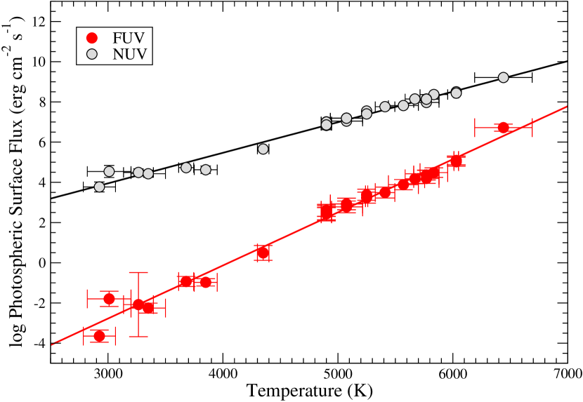
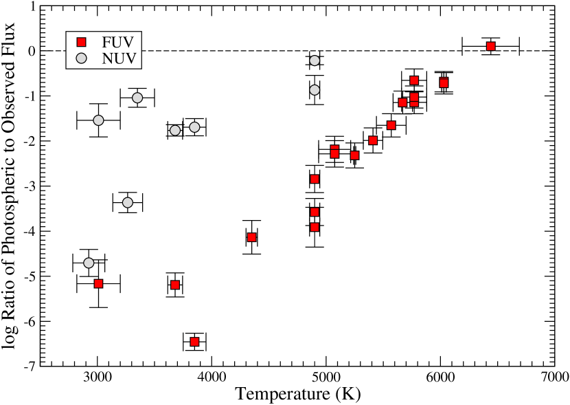
Figure 1: Left: FUV and NUV photospheric surface fluxes as a function of effective temperature for our sample. The M stars (2900 – 4000 K) use main-sequence photospheric fluxes from the Phoenix models while the FGK stars (4000 – 6500 K) use the Kurucz-based values from Findeisen et al. (2011) for which empirically-deduced $T_{\rm eff}$ offsets were applied. The coefficients of the regression analysis are listed in Table 2. Right: Ratio of the photospheric flux to the total observed surface flux for GALEX FUV and NUV bandpasses as a function of temperature.

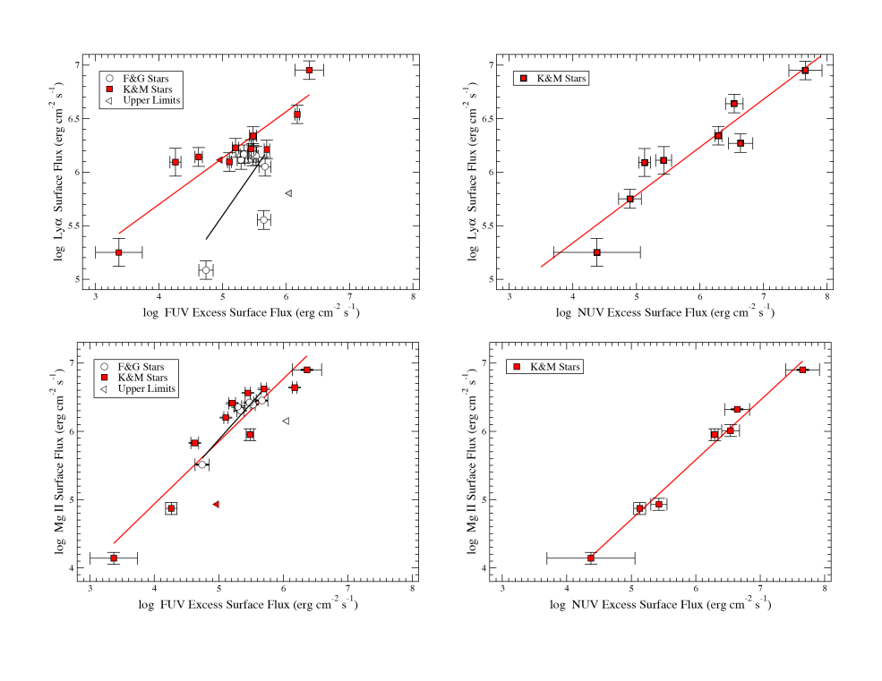
Figure 2: FUV (left column) and NUV (right column) excess surface flux plotted against Lyman $\alpha$  (top row) and Mg II (bottom row) surface flux. Lyman $\alpha$ and Mg II fluxes are taken from Linsky et al. (2013) and scaled to the stellar surface.

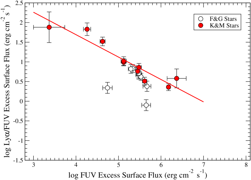
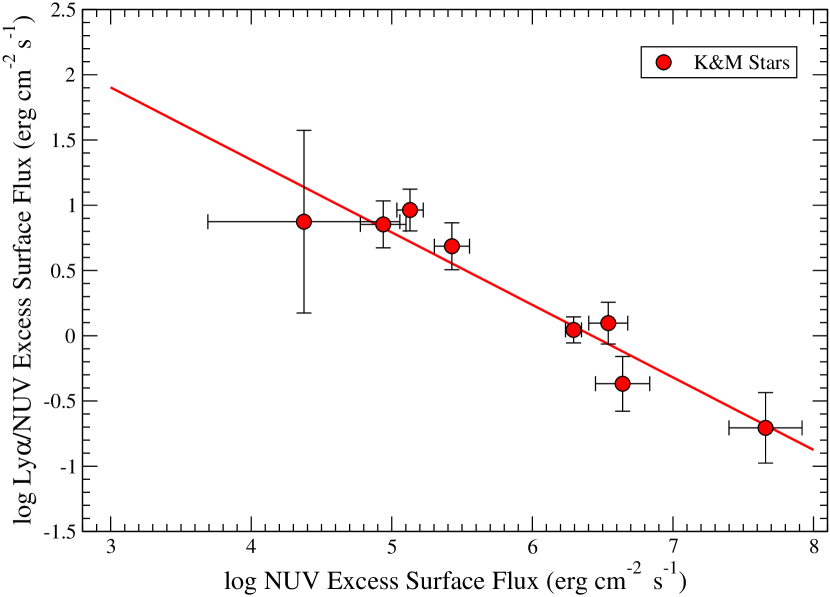
Figure 3: Ratio of Lyman $\alpha$ to FUV (left) and NUV (right) surface flux plotted against the FUV and NUV excess surface flux.

Table 1: Stellar Properties and Surface Line Fluxes

Name	SpT	Dist.	$R_{*}$	$T_{\rm eff}$	log($F_{NUV,obs}$)	log($F_{NUV,exc}$)	log($F_{FUV,obs}$)	log($F_{FUV,exc}$)
		pc	R⊙	K	erg cm-2 s-1	erg cm-2 s-1	erg cm-2 s-1	erg cm-2 s-1
HR 4657	F5 V/L	22.6	1.4	6440	too bright	–	6.62 $\pm$ 0.06	$<$ 6.05
Chi Ori	G0 V	8.7	1.3	6030	too bright	–	not observed	–
HR 4345	G0 V	21.9	1.3	6030	too bright	–	5.77 $\pm$ 0.06	5.67 $\pm$ 0.09
V376 Peg	G0 V	49.6	1.4	6030	too bright	–	5.74 $\pm$ 0.07	5.65 $\pm$ 0.11
HR 2882	G4 V	21.8	1.2	5835	too bright	–	not observed	–
61 Vir	G5 V	8.6	1.4	5770	too bright	–	4.85 $\pm$ 0.07	4.74 $\pm$ 0.11
HR 2225	G5 V	16.7	1.2	5770	too bright	–	5.51 $\pm$ 0.06	5.48 $\pm$ 0.07
HD 203244	G5 V	20.4	1.2	5770	too bright	–	5.38 $\pm$ 0.05	5.34 $\pm$ 0.06
HD 128987	G6 V	23.7	1.1	5670	too bright	–	5.32 $\pm$ 0.05	5.29 $\pm$ 0.06
Xi Boo A	G8 V	6.7	1.1	5570	too bright	–	5.54 $\pm$ 0.03	5.53 $\pm$ 0.04
HD 116956	G9 IV-V	21.9	1.0	5410	too bright	–	5.48 $\pm$ 0.06	5.48 $\pm$ 0.07
DX Leo	K0 V	17.8	0.9	5250	too bright	–	5.70 $\pm$ 0.04	5.70 $\pm$ 0.04
HR 8	K0 V	13.7	1.1	5250	too bright	–	not observed	–
Epsilon Eri	K1 V	3.2	0.9	5075	too bright	–	5.11 $\pm$ 0.03	5.11 $\pm$ 0.03
40 Eri A	K1 V	5.0	1.1	5075	too bright	–	too bright	–
HR 1925	K1 V	12.3	0.9	5075	too bright	–	5.21 $\pm$ 0.05	5.21 $\pm$ 0.05
EP Eri	K2 V	10.4	0.9	4900	too bright	–	5.45 $\pm$ 0.04	5.45 $\pm$ 0.04
LQ Hya	K2 V	18.6	0.9	4900	too bright	–	6.18 $\pm$ 0.04	6.18 $\pm$ 0.04
V368 Cep	K2 V	19.2	1.1	4900	too bright	–	not observed	–
PW And	K2 V	21.9	1.1	4900	7.05 $\pm$ 0.07	6.64 $\pm$ 0.19	not observed	–
Speedy Mic	K2 V/L	52.2	1.1	4900	7.72 $\pm$ 0.22	7.66 $\pm$ 0.26	6.37 $\pm$ 0.22	6.37 $\pm$ 0.22
Epsilon Ind	K5 V	3.6	0.8	4350	too bright	–	4.63 $\pm$ 0.06	4.63 $\pm$ 0.06
AU Mic	M0 V	9.9	1.0	3850	6.30 $\pm$ 0.06	6.29 $\pm$ 0.06	5.48 $\pm$ 0.06	5.48 $\pm$ 0.06
GJ 832	M1.5 V	5.0	0.4	3680	5.28 $\pm$ 0.06	5.13 $\pm$ 0.09	4.26 $\pm$ 0.09	4.26 $\pm$ 0.09
GJ 436	M3 V	10.3	0.2	3350	5.47 $\pm$ 0.11	5.43 $\pm$ 0.13	$<$ 4.97	$<$ 4.97
AD Leo	M3.5 V	4.7	0.3	3265	6.54 $\pm$ 0.14	6.54 $\pm$ 0.14	not observed	–
GJ 876	M5.0 V	4.7	0.3	3010	4.77 $\pm$ 0.21	4.38 $\pm$ 0.68	3.37 $\pm$ 0.37	3.37 $\pm$ 0.37
Proxima Cen	M5.5 V	1.3	0.2	2925	4.93 $\pm$ 0.17	4.90 $\pm$ 0.18	not observed	–

Table 2: Regression Coefficients

Regression Fit	SpT	#	A	B	$R$
	Range
log [$F_{NUV,phot}$] = A $T_{\rm eff}$ + B	F5 V - M5.5 V	28	1.519E–03 $\pm$ 4.080E–05	–0.6094 $\pm$ 0.2063	0.99
log [$F_{FUV,phot}$] = A $T_{\rm eff}$ + B	F5 V - M5.5 V	28	2.640E–03 $\pm$ 6.484E–05	–10.6934 $\pm$ 0.3279	0.99
log [$F_{Ly\alpha}$] = A log [$F_{NUV,obs}$] + B	K2 V - M5.5 V	8	0.430 $\pm$ 0.094	3.595 $\pm$ 0.575	0.88
log [$F_{Ly\alpha}$] = A log [$F_{NUV,exc}$] + B	K2 V - M5.5 V	8	0.447 $\pm$ 0.069	3.549 $\pm$ 0.409	0.94
log [$F_{Ly\alpha}$] = A log [$F_{FUV,exc}$] + B	K0 V - M5.5 V	10	0.432 $\pm$ 0.068	3.969 $\pm$ 0.359	0.91
log [$F_{Ly\alpha}$] = A log [$F_{FUV,exc}$] + B	F5 V - G9 V	8	0.853 $\pm$ 0.427	1.325 $\pm$ 2.307	0.63
log [$F_{Ly\alpha}$/$F_{NUV,exc}$] = A log [$F_{NUV,exc}$] + B	K2 V - M5.5 V	8	–0.556 $\pm$ 0.069	3.570 $\pm$ 0.411	-0.96
log [$F_{Ly\alpha}$/$F_{FUV,exc}$] = A log [$F_{FUV,exc}$] + B	K0 V - M5.5 V	10	–0.570 $\pm$ 0.071	3.970 $\pm$ 0.374	-0.94
log [$F_{Ly\alpha}$/$F_{FUV,exc}$] = A log [$F_{FUV,exc}$] + B	F5 V - G9 V	8	no corr.	–	–
log [$F_{MgII}$] = A log [$F_{NUV,exc}$] + B	K2 V - M5.5 V	7	0.872 $\pm$ 0.049	0.349 $\pm$ 0.301	0.99
log [$F_{MgII}$] = A log [$F_{FUV,exc}$] + B	K0 V - M5.5 V	10	0.916 $\pm$ 0.116	1.272 $\pm$ 0.610	0.94
log [$F_{MgII}$] = A log [$F_{FUV,exc}$] + B	F5 V - G9 V	6	1.056 $\pm$ 0.177	0.599 $\pm$ 0.946	0.95

References

- Baraffe et al. (1998) Baraffe, I., Chabrier, G., Allard, F., & Hauschildt, P. H. 1998, A&A, 337, 403
- Claire et al. (2012) Claire, M. W., Sheets, J., Cohen, M., Ribas, I., Meadows, V. S., & Catling, D. C. 2012, ApJ, 757, 95
- Correia et al. (2010) Correia, A. C. M., et al. 2010, A&A, 511, A21
- Findeisen & Hillenbrand (2010) Findeisen, K., & Hillenbrand, L. 2010, AJ, 139, 1338
- Findeisen et al. (2011) Findeisen, K., Hillenbrand, L., & Soderblom, D. 2011, AJ, 142, 23
- Fontenla et al. (1988) Fontenla, J., Reichmann, E. J., & Tandberg-Hanssen, E. 1988, ApJ, 329, 464
- France et al. (2013) France, K., et al. 2013, ApJ, 763, 149
- France et al. (2012) France, K., Linsky, J. L., Tian, F., Froning, C. S., & Roberge, A. 2012, ApJ, 750, L32
- Hauschildt et al. (1997) Hauschildt, P. H., Baron, E., & Allard, F. 1997, ApJ, 483, 390
- Heller & Armstrong (2014) Heller, R., & Armstrong, J. 2014, Astrobiology, 14, 50
- Hu et al. (2012) Hu, R., Seager, S., & Bains, W. 2012, ApJ, 761, 166
- Kasting et al. (1993) Kasting, J. F., Whitmire, D. P., & Reynolds, R. T. 1993, Icarus, 101, 108
- Kopparapu et al. (2012) Kopparapu, R. k., Kasting, J. F., & Zahnle, K. J. 2012, ApJ, 745, 77
- Kraus & Hillenbrand (2007) Kraus, A. L., & Hillenbrand, L. A. 2007, AJ, 134, 2340
- Kraus et al. (2014) Kraus, A. L., Shkolnik, E. L., Allers, K. N., & Liu, M. C. 2014, AJ, 147, 146
- Lammer et al. (2007) Lammer, H., et al. 2007, Astrobiology, 7, 185
- Linsky et al. (2013) Linsky, J. L., France, K., & Ayres, T. 2013, ApJ, 766, 69
- Miguel & Kaltenegger (2014) Miguel, Y., & Kaltenegger, L. 2014, ApJ, 780, 166
- Miguel et al. (2014) Miguel, Y., Kaltenegger, L., Linsky, J. L., & Rugheimer, S. 2014, ArXiv e-prints
- Morrissey et al. (2007) Morrissey, P., et al. 2007, ApJS, 173, 682
- Morrissey et al. (2005) —. 2005, ApJ, 619, L7
- Ochsenbein et al. (2000) Ochsenbein, F., Bauer, P., & Marcout, J. 2000, A&AS, 143, 23
- Pagano (2009) Pagano, I. 2009, Ap&SS, 320, 115
- Preibisch & Feigelson (2005) Preibisch, T., & Feigelson, E. D. 2005, ApJS, 160, 390
- Ribas et al. (2005) Ribas, I., Guinan, E. F., Güdel, M., & Audard, M. 2005, ApJ, 622, 680
- Robinson et al. (2005) Robinson, R. D., et al. 2005, ApJ, 633, 447
- Rodriguez et al. (2011) Rodriguez, D. R., Bessell, M. S., Zuckerman, B., & Kastner, J. H. 2011, ApJ, 727, 62
- Scalo et al. (2007) Scalo, J., et al. 2007, Astrobiology, 7, 85
- Shkolnik (2013) Shkolnik, E. L. 2013, ApJ, 766, 9
- Shkolnik & Barman (2014) Shkolnik, E. L., & Barman, T. S. 2014, ArXiv e-prints
- Shkolnik et al. (2011) Shkolnik, E. L., Liu, M. C., Reid, I. N., Dupuy, T., & Weinberger, A. J. 2011, ApJ, 727, 6, 12 pp
- Short & Hauschildt (2005) Short, C. I., & Hauschildt, P. H. 2005, ApJ, 618, 926
- Smith & Redenbaugh (2010) Smith, G. H., & Redenbaugh, A. K. 2010, PASP, 122, 1303
- Tarter et al. (2007) Tarter, J. C., et al. 2007, Astrobiology, 7, 30
- Tian et al. (2014) Tian, F., France, K., Linsky, J. L., Mauas, P. J. D., & Vieytes, M. C. 2014, Earth and Planetary Science Letters, 385, 22
- Walkowicz & Hawley (2009) Walkowicz, L. M., & Hawley, S. L. 2009, AJ, 137, 3297
- Welsh et al. (2006) Welsh, B. Y., et al. 2006, A&A, 458, 921
- Wood et al. (2005) Wood, B. E., Redfield, S., Linsky, J. L., Müller, H.-R., & Zank, G. P. 2005, ApJS, 159, 118
- Wu & Lithwick (2013) Wu, Y., & Lithwick, Y. 2013, ApJ, 772, 74, 13 pp