Exponential Asymptotics and Stokes Line Smoothing for Generalized Solitary Waves

Abstract. 

In a companion paper, Grimshaw (Asymptotic Methods in Fluid Mechanics, 2010, pp. 71–120) has demonstrated how techniques of Borel summation can be used to elucidate the exponentially small terms that lie hidden beyond all orders of a divergent asymptotic expansion. Here, we provide an alternative derivation of the generalized solitary waves of the fifth-order Korteweg-de Vries equation. We will first optimally truncate the asymptotic series, and then smooth the Stokes line. Our method provides an explicit view of the switching-on mechanism, and thus increased understanding of the Stokes Phenomenon.

Chapter 1 Introduction

The Stokes Phenomenon describes the puzzling event in which exponentially small terms can suddenly appear or disappear when an asymptotic expansion is analytically continued across key lines (Stokes lines) in the Argand plane—“as it were into a mist,” Stokes once remarked in 1902.

Fortunately, much of the inherent vagueness of this phenomenon, as well as its deep implications for the study of asymptotic approximations has been examined since Stokes’ time (see Boyd (1999) for a comprehensive review). In another paper of this volume by Grimshaw (2011)—henceforth referred to as [Grimshaw]—it was shown how Borel summation can be used to reveal the exponentially small waves found in the fifth-order Korteweg-de Vries equation (5KdV).

In this review paper, we will show how the methodology outlined in Olde Daalhuis et al. (1995) and Chapman et al. (1998) can be used as an alternative treatment of the 5KdV equation. The procedure is as follows: (1) Expand the solution as a typical asymptotic expansion, (2) find the behaviour of the late-order terms ($n\to\infty$), and (3) optimally truncate the expansion and examine the remainder as the Stokes lines are crossed.

The location of the Stokes lines, as well as the details of the Stokes Phenomenon and resultant exponentials are intrinsically linked to the late- order terms of the asymptotic approximation—thus, as we proceed through Steps 1 to 3, we are effectively deriving the beyond-all-orders contributions by decoding the divergent tails of the expansion. The novelty in this approach (in contrast to the one shown in [Grimshaw]) is that all the analysis is done in the (complexified) physical space, rather than in Borel-transformed space. This provides us with a special vantage point—to see the smooth switching-on of the exponentially small terms as each Stokes line is crossed (see Figure 1). Come, let us stare into Stokes’ mist.

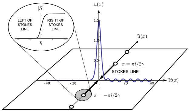
Figure 1: The analytic continuation of the traditional asymptotic solution (the classical solitary wave) contains singularities up and down the imaginary axis, with Stokes lines emanating from each of these singularities. By re-scaling near the singularities and optimally truncating, we will be able to observe the smooth switching-on of the exponentially small terms (top-left).

Chapter 2 Generalized Solitary Waves and the 5KdV

We will consider the existence of solutions to the 5KdV equation,

$$\epsilon^{2}u_{xxxx}+u_{xx}+3u^{2}-cu=0$$ (1)

with $u\to 0$ as $x\to\pm\infty$. Although the problem is for $x\in\mathbb{R}$, it will be important to consider the effects of allowing $u$ and $x$ to be complex.

1 Initial Asymptotic Analysis and Late Terms

We begin as usual by substituting the asymptotic expansions,

$$u=\sum_{n=0}^{\infty}\epsilon^{2n}u_{n}\text{\quad and \quad}c=\sum_{n=0}^{\infty}\epsilon^{2n}c_{n}$$

into Equation (1). This yields the first two orders as,

$$u_{0} =2\gamma^{2}\textrm{sech}^{2}(\gamma x) c_{0} =4\gamma^{2}$$ (2)

$$u_{1} =-10\gamma^{2}u_{0}+\left(\frac{15}{2}\right)u_{0}^{2} c_{1} =c_{0}^{2}$$ (3)

while at $O(\epsilon^{2n})$,

$$u_{(n-1)xxxx}+u_{nxx}+6u_{0}u_{n}-c_{0}u_{n}+\ldots=0.$$ (4)

Here, the key observation is that there exists singularities in the analytic continuation of the leading order solution, $u_{0}(x)$ at $x=\pm\pi i/2\gamma,\pm 3\pi i/2\gamma,\ldots$ This use of ill-defined approximations in order to represent perfectly well-defined phenomena is one of the caveats of singular asymptotics, but one would feverishly hope that a singularity far from the region of interest (in this case, $x\in\mathbb{R}$) has little effect on the approximations!

Unfortunately this is not the case. We see from Equation (4) that at each order, $u_{n}$ is partly determined by differentiating $u_{n-1}$ twice and thus each additional order adds to the power of the singularities in the early terms. We would therefore expect the late terms of the asymptotic expansion to exhibit factorial over power divergence of the form,

$$u_{n}\sim\frac{Q(z)\Gamma(2n+\gamma)}{[\chi(z)]^{2n+\gamma}},\quad\text{as $n\to\infty$.}$$ (5)

Here, $\gamma$ is a constant, while $Q(z)$ and $\chi(z)$ are functions to be determined. Substituting this ansatz into Equation (4) yields at leading order,

$$-\left(\frac{d\chi}{dz}\right)^{4}+\left(\frac{d\chi}{dz}\right)^{2}=0,\quad\text{as $n\to\infty$.}$$ (6)

Now from the above discussion, we would expect that $\chi=0$ at the relevant singularities, $x=\sigma_{i}$ for some $i$; we then conclude that $\chi^{\prime}=\pm 1$ and thus without loss of generality, $\chi=x-\sigma_{i}$. In general, $u_{n}$ will be a sum of terms of the form (5), one for each singularity. However along the real axis, the behaviour of $u_{n}$ will be dominated by those singularities closest to the axis and thus we need only concern ourselves with the singularities at $x=\pm\sigma\equiv\pm i\pi/2\gamma$. Finally, at next order as $n\to\infty$, we find that $Q(z)=\Lambda$, a constant.

The determination of $\gamma$, $\Lambda$, and in fact, the Stokes line smoothing in the next section will require an analysis near each of the two singularities, $x=\pm\sigma$; for brevity, we will henceforth focus on the singularity at $x=\sigma$ in the upper-half plane.

First, since by Equation (2), $u_{0}\sim-2/(x-\sigma)^{2}$ as $x\to\sigma$, we must require that $\gamma=2$. Second, in order to determine the final constant $\Lambda$, we need to re-scale near the singularity $x=\sigma$, express the leading-order inner solution as a power series (in inner coordinates) and match with the outer solutions. In the end, however, $\Lambda$ is determined by the numerical solution of a canonical inner problem. As was shown in [Grimshaw], $\Lambda\approx-19.97$.

Finally, let us discuss the significance of $\chi$. Following Dingle (1973), we expect there to be a Stokes line wherever $u_{n}$ and $u_{n+1}$ have the same phase as $n\to\infty$, or in this case where,

$$\Im\left[-\chi^{2}\right]=0\text{ and }\Re\left[-\chi^{2}\right]\geq 0.$$ (7)

Thus there exist Stokes lines from $x=\pi i/2\gamma$ down the imaginary axis and from $x=-\pi i/2\gamma$ up the imaginary axis (as illustrated in Figure 1). In the next section, we will optimally truncate the asymptotic expansion and examine the switching-on of exponentially small terms as these two Stokes lines are crossed.

2 Optimal Truncation and Stokes Smoothing

By now we have entirely determined the late terms of the asymptotic expansion. In order to identify the exponentially small waves, we truncate the expansion and study its remainder,

$$u=\sum_{n=0}^{N-1}\epsilon^{2n}u_{n}+R_{N}(x).$$

Substitution into Equation (1) yields the equation

$$\epsilon^{2}R_{N}^{\prime\prime\prime\prime}+R_{N}^{\prime\prime}+6u_{0}R_{N}-c_{0}R_{N}+\ldots\sim\epsilon^{2N}u_{N}^{\prime\prime},$$ (8)

which, using Stirling’s formula, we can write the right-hand side as

$$\epsilon^{2N}u_{N}^{\prime\prime}\sim\epsilon^{2N}\frac{\Lambda(-1)^{N}\Gamma(2N+\gamma+2)\chi^{\prime}}{\chi^{2N+\gamma+2}}\\ \sim\epsilon^{2N}\frac{\Lambda(-1)^{N}\left\{\sqrt{2\pi}e^{-(2N+\gamma+2)}(2N+\gamma+2)^{2N+\gamma+3/2}\right\}}{\chi^{2N+\gamma+2}}$$ (9)

We can see now that the remainder is only algebraically small unless $N\sim\lvert\chi\rvert/2\epsilon$ (where the ratio of consecutive terms are equal) and thus we set $N=r/2\epsilon+\rho$ where $\rho$ is bounded as $\epsilon\to 0$.

Although there are four homogeneous solutions to Equation (8) as $\epsilon\to 0$, we will show that one in particular,

$$R_{N}(x)\sim S(x)e^{-i(x-\sigma)/\epsilon}$$ (10)

is switched on as the Stokes line is crossed. We will call the function $S(x)$ the Stokes multiplier, and we expect it to vary smoothly from one constant to another across the Stokes line. We write

$$\chi=x-\sigma=re^{i\theta}\text{\quad and \quad}\frac{d}{dx}=-\frac{ie^{-i\theta}}{r}\frac{d}{d\theta},$$ (11)

where now, since $N$ is fixed (and thus also the modulus, $r$), we are only interested in the “fast” variation in $\theta$ across the Stokes line. Then using Equations (9) and (11) in (8) gives

$$\frac{dS}{d\theta}\sim\frac{\Lambda\sqrt{r\pi}}{\sqrt{2}\epsilon^{\gamma+1/2}}\ e^{-r/\epsilon}e^{ire^{i\theta}/\epsilon}\Bigl{(}e^{-i\theta}\Bigr{)}^{r/\epsilon+2\rho+\gamma+2}\Bigl{(}e^{-\pi i/2}\Bigr{)}^{r/\epsilon+2\rho}e^{i\theta}\\ =\frac{\Lambda\sqrt{r\pi}}{\sqrt{2}\epsilon^{\gamma+1/2}}\times\exp\left[-\frac{r}{\epsilon}\left\{1-ie^{i\theta}+i\theta+\frac{\pi i}{2}\right\}\right.\\ \left.+i\left\{-2\rho\left(\theta+\frac{\pi}{2}\right)-\theta(\gamma+1)\right\}\right]$$ (12)

From the terms within the curly braces, we see that the change in $S$ is exponentially small, except near the Stokes line $\theta=-\pi/2$. Here, we will re-scale $\theta=-\pi/2+\sqrt{\epsilon}\eta$ and integrate Equation (12) from left ($\eta\to-\infty$) to right to show that

$$S\sim\text{const}+\frac{\Lambda\sqrt{\pi}}{\sqrt{2}\epsilon^{\gamma}}e^{\pi i(\gamma+1)/2}\int_{-\infty}^{\sqrt{r}\eta}e^{-s^{2}/2}\ ds.$$ (13)

This integral (the error function) precisely illustrates the smoothing of the Stokes line in Figure 1. Thus the jump in the Stokes multiplier and consequently, the remainder is

$$\Bigl{[}S\Bigr{]}_{\text{Stokes}}\sim\frac{\Lambda\pi}{\epsilon^{\gamma}}e^{3\pi i/2}\Longrightarrow\Bigl{[}R_{N}\Bigr{]}_{\text{Stokes}}\sim\frac{\Lambda\pi}{\epsilon^{2}}e^{3\pi i/2}e^{-i(x-\sigma)/\epsilon}.$$ (14)

We must remember that the analysis must be repeated for analytic continuation into the lower-half $x$-plane and thus near the singularity at $x=-\pi i/2\gamma$. The result is another exponentially small contribution which is the complex conjugate of Equation (14) and thus along the real axis, the sum of contributions from crossing the pair of Stokes lines is,

$$u_{\text{exp}}\sim-\frac{2\Lambda\pi}{\epsilon^{2}}e^{-\pi/2\gamma\epsilon}\sin\left(x/\epsilon\right).$$ (15)

Let us recap our analysis: (1) The singular nature of the 5KdV equation produces singularities in the early terms, (2) As more and more terms are taken, the effects of the singularities grow, eventually producing factorial over power divergence in the late terms, (3) Stokes lines emerge from each of the singularities, and (4) By optimally truncation and examining the jump in the remainder as the Stokes lines are crossed, we see the Stokes Phenomenon and thus the appearance of exponentially small terms.

So finally, we are ready to answer the original question: Do there exist classical solitary wave solutions of the 5KdV equation? No. For suppose that we did impose the condition that only the base (non-oscillatory) asymptotic solution applies at $x=-\infty$. Then as we pass through $x=0$, the term in Equation (15) necessarily switches on and $u\sim u_{0}+u_{\text{exp}}$ for $x>0$.

We have thus passed through Stokes’ mist and subsequently, realized that there do not exist classical solitary wave solutions of the 5KdV.

References

- Boyd (1999) J.P. Boyd. The Devil’s invention: Asymptotics, superasymptotics and hyperasymptotics. Acta Applicandae, 56:1–98, 1999.
- Chapman et al. (1998) S.J. Chapman, J.R. King, and K.L. Adams. Exponential asymptotics and Stokes lines in nonlinear ordinary differential equations. Proc. R. Soc. Lond. A, 454:2733–2755, 1998.
- Dingle (1973) R.B. Dingle. Asymptotic Expansions: Their Derivation and Interpretation. Academic Press, London, 1973.
- Olde Daalhuis et al. (1995) A.B. Olde Daalhuis, S.J. Chapman, J.R. King, J.R. Ockendon, and R.H. Tew. Stokes Phenomenon and matched asymptotic expansions. SIAM J. Appl. Math., 55(6):1469–1483, 1995.
- Stokes (1902) G.G. Stokes. On the discontinuity of arbitrary constants that appear as multiples of semi-convergent series. Acta. Math. Stockholm, 26:393–397, 1902.
- Grimshaw (2011) R. Grimshaw. Exponential asymptotics and generalized solitary waves. In Asymptotic Methods in Fluid Mechanics: Survey and Recent Advances (ed. Steinrück H.), Springer:1–98, 2011.