NLTE effects on the iron abundance of AGB stars in 47 Tucanae

Abstract

We present the iron abundance of 24 asymptotic giant branch (AGB) stars members of the globular cluster 47 Tucanae, obtained with high-resolution spectra collected with the FEROS spectrograph at the MPG/ESO-2.2m Telescope. We find that the iron abundances derived from neutral lines (with mean value [Fe I/H]$=-0.94\pm 0.01$, $\sigma=0.08$ dex) are systematically lower than those derived from single ionized lines ([Fe II/H]$=-0.83\pm 0.01$, $\sigma=0.05$ dex). Only the latter are in agreement with those obtained for a sample of red giant branch (RGB) cluster stars, for which Fe I and Fe II lines provide the same iron abundance. This finding suggests that Non Local Thermodynamical Equilibrium (NLTE) effects driven by overionization mechanisms are present in the atmosphere of AGB stars and significantly affect Fe I lines, while leaving Fe II features unaltered. On the other hand, the very good ionization equilibrium found for RGB stars indicates that these NLTE effects may depend on the evolutionary stage. We discuss the impact of this finding both on the chemical analysis of AGB stars, and on the search for evolved blue stragglers.

1 Introduction

The asymptotic giant branch (AGB) evolutionary phase is the final stage of thermonuclear burning for low/intermediate mass stars (M $<$ 8 $M_{\odot}$). AGB stars are known to dominate the integrated light of intermediate age stellar systems (see, e.g., Renzini & Buzzoni, 1986; Ferraro et al., 1995; Hoefner et al., 1998; van Loon et al., 1999; Cioni & Habing, 2003; Maraston, 2005) and to play a crucial role in the chemical enrichment processes of cosmic structures. In fact, from one side they are the main sites where elements heavier than the Fe-peak (like Ba and La) are formed, through slow neutron captures (Busso et al., 1999), and promptly ejected. On the other side, their interiors can reach temperatures high enough to activate the proton-capture reaction chains, like the NeNa and the MgAl ones. Intermediate-mass AGB stars are also considered to be responsible for the chemical anomalies (involving C, N, O, Na, Mg and Al) detected in all properly observed Galactic globular clusters (GCs; see Gratton et al., 2012) and in old Magellanic Cloud globulars (Mucciarelli et al., 2009).

Due to their short lifetimes (of the order of $\sim$10 Myr for a low-mass star with 0.8 $M_{\odot}$), the number of AGB stars observable in an old GC is small, about a factor of 3-4 smaller than the number of red giant branch (RGB) stars of comparable luminosity. Additionally, high-quality photometry and large color baselines are needed to properly separate genuine AGB from RGB stars. Hence, despite their luminosity, these objects are still not well investigated from the chemical point of view. Accurate determinations of their atmospheric parameters and metallicity based on high-resolution spectroscopy are available for a few GCs only, namely M 4 (Ivans et al., 1999), M 5 (Ivans et al., 2001; Koch & McWilliam, 2010) and 47 Tucanae (hereafter 47Tuc, Wylie et al., 2006; Koch & McWilliam, 2008; Worley et al., 2009), and they are all based on small samples (no more than 6 AGB stars in each of the quoted clusters). Particular care has been addressed to the different distribution of CN (Mallia, 1978; Norris et al., 1981; Briley et al., 1993) and Na (Campbell et al., 2013) in AGB and RGB stars, in light of the self-enrichment processes predicted to occur in the early stage of GC life (see e.g. D’Ercole et al., 2008).

New interest for AGB stars has been raised in a different research field from the observational results of Beccari et al. (2006), who found a significant excess ($\sim 30\%$) and an anomalous segregation of such objects in the central regions of 47 Tucanae (see also Dalessandro et al. 2009 for the case of M 2). This finding suggests that the genuine AGB population of this GC may be “contaminated” by a peculiar class of heavy intruders, namely the descendants of blue straggler stars experiencing their giant evolutionary phases (hereafter, evolved blue straggler stars, e-BSSs). While confirming such a hypothesis would provide precious constraints to the evolutionary models of these exotica, no firm identification of even a single e-BSS has been obtained to date. Indeed, a detailed investigation of AGB stars could finally fill this gap.

In this paper we present the determination of the iron abundance for a sample of 24 AGB stars in the metal-rich Galactic GC 47 Tuc. The observations and the spectroscopic analysis are described in Section 2 and 3, respectively. Section 4 presents the measured iron abundances and a series of tests demonstrating the correctness of the adopted procedure and assumptions. A discussion of the results obtained and of their impact on the traditional chemical analysis and the search for e-BSSs is provided in Section 5. The conclusions of the work are summarized in Section 6.

2 Observations

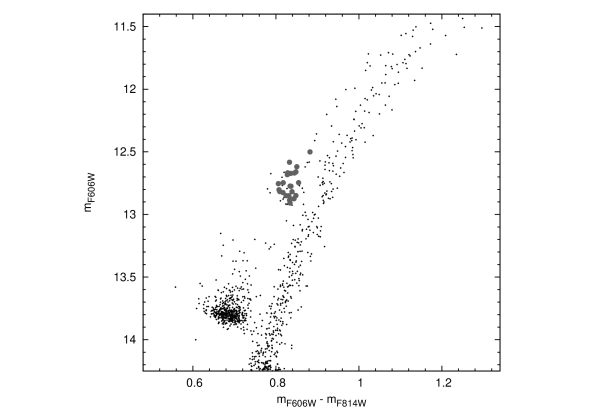
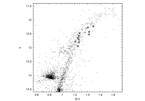
Figure 1: Top panel: $(m_{\rm F606W},m_{\rm F606W}-m_{\rm F814W})$ color magnitude diagram of 47 Tuc from Beccari et al. (2006). The large solid circles mark the 24 targets studied in the present work. Bottom panel: ($V,V-I$) color magnitude diagram of 47 Tuc obtained from WFI data by Ferraro et al. (2004). The large solid squares mark the 11 RGB stars used for comparison.

We acquired high resolution spectra of 24 AGB stars in 47 Tuc (Program ID 090.D-0153, PI: Lanzoni) by using the Fibre-fed Extended Range Optical Spectrograph (FEROS; Kaufer et al., 1999) mounted at the MPG/ESO-2.2m telescope. The spectra cover a wavelength range between $\lambda\sim 3500~{}\mathring{\rm A}$ and $\lambda\sim 9200~{}\mathring{\rm A}$, with a spectral resolution of $\sim 48000$. FEROS allows to allocate simultaneously two fibers at a relative distance of $2.9\arcmin$, one on the source and the other on the sky. The targets have been selected from the photometric catalog of Beccari et al. (2006), within $\sim 100\arcsec$ from the cluster center. In the color-magnitude diagram (CMD) of 47 Tuc they are located in the AGB clump (corresponding to the beginning of this evolutionary phase; Ferraro et al., 1999), at $m_{\rm F606W}\sim 12.8$ and $(m_{\rm F606W}-m_{\rm F814W})\simeq 0.8$ (see top panel of Figure 1). Only isolated stars have been selected, in order to avoid contamination of the spectra from close objects of larger or comparable luminosity. The identification number, coordinates and magnitudes of each target are listed in Table 1.

For each target a single exposure of $\sim$30-40 min has been acquired, reaching signal-to-noise ratios S/N$\geq 70$ per pixel. The data reduction was performed by using the ESO FEROS pipeline, including bias subtraction, flat fielding, wavelength calibration by using a Th-Ar-Ne reference lamp, spectrum extraction and final merging and rebinning of the orders. Since the background level of the sky is negligible ($<1\%$) compared to the brightness of the observed targets, we did not perform the sky subtraction from the final spectra in order to preserve its maximum quality. We accurately checked that the lack of sky subtraction has no impact on the derived abundances, by comparing the equivalent widths (EWs) measured for some spectra with and without the sky subtraction.

3 Analysis

3.1 Radial velocities

The radial velocity of each target has been obtained by means of the code DAOSPEC (Stetson & Pancino, 2008), measuring the positions of more than 300 metallic lines. The accuracy of the wavelength calibration has been checked by measuring telluric absorptions and oxygen sky lines, finding no significant zero-point offsets. Uncertainties have been computed as the dispersion of the measured radial velocities divided by the square root of the number of used lines, and they turned out to be smaller than 0.04 km s^-1. Heliocentric corrections obtained with the IRAF task RVCORRECT have been adopted. The heliocentric radial velocities for all the targets are listed in Table 1. They range between $\sim-41.5$ and $\sim+9.5$ km s^-1, with mean value of $-17.6\pm 2.3$ km s^-1 and dispersion $\sigma=11.5$ km s^-1. These values are in good agreement with previous determinations of the systemic radial velocity of 47 Tuc (see e.g. Mayor et al., 1983; Meylan et al., 1991; Gebhardt et al., 1995; Carretta et al., 2004; Alves-Brito et al., 2005; Koch & McWilliam, 2008; Lane et al., 2010). All the targets have been considered as members of the cluster, according to their radial velocities and distance from the cluster center.

3.2 Chemical analysis

The chemical abundances have been derived by using the package GALA (Mucciarelli et al., 2013a) which matches the measured and the theoretical equivalent widths (see Castelli, 2005, for a detailed description of this method). The model atmospheres have been computed by using the ATLAS9 code, under the assumption of plane-parallel geometry, local thermodynamical equilibrium (LTE) and no overshooting in the computation of the convective flux. We adopted the last release of the opacity distribution functions from Castelli & Kurucz (2004), assuming a global metallicity of [M/H] = $-1$ dex with [$\alpha$/Fe]$=+0.4$ dex for the model atmospheres.

The effective temperatures ($T_{\rm eff}$) and surface gravities ($\log g$) of the targets have been derived photometrically, by projecting the position of each star in the CMD onto the isochrone best fitting the main evolutionary sequences of 47 Tuc. The isochrone has been extracted from the BaSTI database (Pietrinferni et al., 2006) assuming an age of 12 Gyr, metallicity Z $=0.008$ and $\alpha$-enhanced chemical mixture. We adopted a distance modulus $(m-M)_{V}=13.32$ mag and a color excess $E(B-V)=0.04$ mag (Ferraro et al., 1999). Microturbulent velocities ($v_{\rm turb}$) have been derived by requiring that no trends exist between Fe I abundances and the reduced EWs, defined as $\log(EW/\lambda)$. The adopted atmospheric parameters are listed in Table 2.

Only absorption lines that are predicted to be unblended at the FEROS resolution have been included in our analysis. The line selection has been performed through a careful inspection of synthetic spectra calculated with the code SYNTHE (Sbordone et al., 2005) assuming the typical atmospheric parameters of our targets and the typical metallicity of 47 Tuc. We considered only transitions with accurate theoretical/laboratory atomic data taken from the last version of the Kurucz/Castelli compilation. The EWs have been obtained with DAOSPEC (Stetson & Pancino, 2008), iteratively launched by means of the package 4DAO(Mucciarelli, 2013) that allows an analysis cascade of a large sample of stellar spectra and a visual inspection of the Gaussian fit obtained for all the investigated lines. Due to the extreme crowding of spectral lines in the region between $\lambda\sim 3800~{}\mathring{\rm A}$ and $\lambda\sim 4500~{}\mathring{\rm A}$, and to the presence of several absorption telluric line bands beyond $\sim 6800~{}\mathring{\rm A}$, we restricted the analysis to the spectral range between $\sim 4500~{}\mathring{\rm A}$ and $\sim 6800~{}\mathring{\rm A}$. In order to avoid too weak or saturated features, we considered only lines with reduced EWs between $-5.6$ and $-4.7$ (these correspond to EW = 11 m$\mathring{\rm A}$ and 90 m$\mathring{\rm A}$ at $\lambda\sim 4500~{}\mathring{\rm A}$, and EW = 17 m$\rm\mathring{A}$ and 135 m$\rm\mathring{A}$ at $\lambda\sim 6800~{}\mathring{\rm A}$, respectively). Moreover, we discarded from the analysis also the lines with EW uncertainties larger than $20\%$, where the uncertainty of each individual line is provided by DAOSPEC on the basis of the fit residuals. With these limitations, the iron abundance has been derived, on average, from $\sim 150$ Fe I lines and $\sim 13$ Fe II lines. In the computation of the final iron abundances we adopted as reference solar value A(Fe)_⊙ = 7.50 dex (Grevesse & Sauval, 1998).

Uncertainties on the derived abundances have been computed for each target by adding in quadrature the two main error sources: (a) those arising from the EW measurements, which have been estimated as the line-to-line abundance scatter divided by the square root of the number of lines used, and (b) the uncertainties arising from the atmospheric parameters, computed varying by the corresponding uncertainty only one parameter at a time, while keeping the others fixed. The abundance variations thus obtained have been added in quadrature. Term (a) is of the order of less than 0.01 dex for Fe I and 0.03 dex for Fe II. Since the atmospheric parameters have been estimated from photometry, by projecting the position of each target in the CMD onto the isochrone, we estimated term (b) from the photometric uncertainties. By assuming a conservative uncertainty of 0.1 mag for the magnitudes of our targets we obtained an uncertainty of about $\pm$50 K and $\pm$0.05 dex on the final T_eff and log $g$, respectively. The total uncertainties in [Fe I/H] are of the order of 0.04-0.05 dex, while in [Fe II/H] are of about 0.08-0.10 dex (due to the higher sensitivity of Fe II lines to $T_{\rm eff}$ and $\log g$).

4 Iron abundance

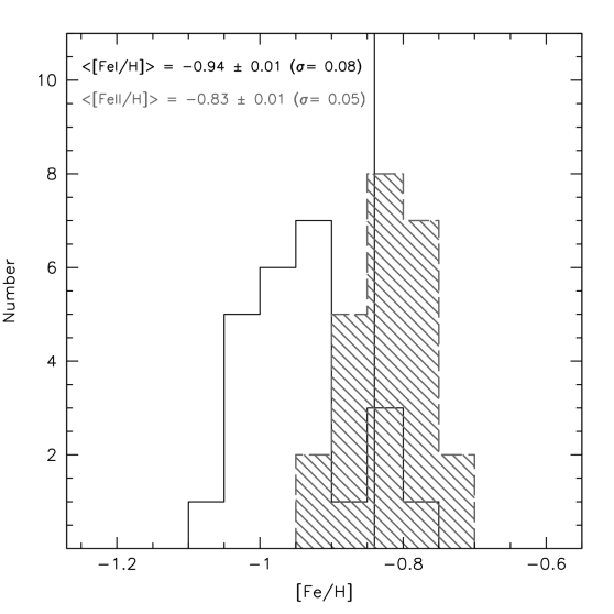
Figure 2: Distribution of the iron abundance ratios measured for the 24 AGB stars in our sample, from Fe I lines (empty histogram) and from Fe II lines (shaded histogram). The vertical line indicates the average iron abundance derived from 11 RGB stars.

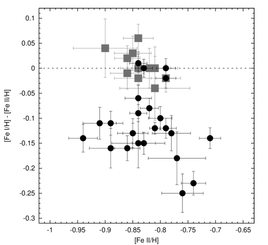
Figure 3: Difference between [Fe I/H] and [Fe II/H] as a function of [Fe II/H] for the 24 AGB stars (black circles) and the 11 RGB stars (gray squares) in our 47 Tuc samples.

The [Fe I/H] and [Fe II/H] abundance ratios measured for each target are listed in Table 2, together with the total uncertainties and the number of lines used. Their distributions are shown in Figure 2. A systematic difference between [Fe I/H] and [Fe II/H] is evident, with the abundances derived from Fe I lines being, on average, $0.1$ dex smaller than those obtained from Fe II: the mean values of the distributions are [Fe I/H] $=-0.94\pm 0.01$ ($\sigma=0.08$ dex) and [Fe II/H] $=-0.83\pm 0.01$ ($\sigma=0.05$ dex). These values are clearly incompatible each other. Moreover, only [FeII/H] is in agreement with the metallicity quoted in the literature and based on sub-giant or RGB stars (Carretta et al., 2004; Alves-Brito et al., 2005; Koch & McWilliam, 2008; Carretta et al., 2009), while the iron abundance obtained from Fe I lines is significantly smaller. The distribution of the difference [Fe I/H]$-$[Fe II/H] is shown as a function of [Fe II/H] in Figure 3 (black circles). It is quite broad, ranging from $-0.25$ to $+0.01$ dex.

4.1 Sanity checks

The difference in the derived [Fe I/H] and [Fe II/H] abundances cannot be easily explained (especially if considering the high quality of the acquired spectra and the very large number of used iron lines) and it clearly needs to be understood. In order to test the correctness of our analysis and to exclude possible bias or systematic effects, we therefore performed a number of sanity checks.

4.1.1 Checks on the chemical analysis procedure

To test the reliability of our chemical analysis, we studied a sample of RGB stars in 47 Tuc, the standard star 104 Tau, Arcturus and the Sun by following the same procedure adopted for the AGB targets discussed above (i.e., by using the same linelist, model atmospheres, and method to infer the atmospheric parameters).

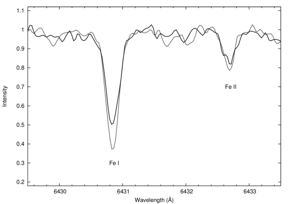
Figure 4: Comparison between the normalized spectra of target #100171 (grey line) and #100174 (black line). The position of a Fe I line and a Fe II line is marked.

RGB stars in 47 Tuc – We measured the iron abundance for a sample of 11 RGB stars in 47 Tuc, for which high-resolution (R$\sim$45000) FLAMES-UVES spectra are available in the ESO Archive (Program ID: 073.D-0211). The location of these stars in the ($V$,$V-I$) CMD from Ferraro et al. (2004) is shown in Figure 1 (bottom panel). Their atmospheric parameters and [Fe I/H] and [Fe II/H] abundance ratios are listed in Table 3. The distribution of the [Fe I/H]-[Fe II/H] differences is shown in Figure 4 (large gray squares). We found an average [Fe I/H]${}_{\rm RGB}=-0.83\pm 0.01$ dex ($\sigma=0.02$ dex) and [Fe II/H]${}_{\rm RGB}=-0.84\pm 0.01$ dex ($\sigma=0.03$ dex). These values are fully consistent with previous determinations. In fact, the careful comparison with the results of Carretta et al. (2009), who analyzed the same 11 RGB spectra, shows that the average differences in the adopted parameters are: $\Delta T_{\rm eff}=36\pm 8$ K ($\sigma$ = 26 K), $\Delta\log g=0.07\pm 0.01$ ($\sigma$ = 0.04), $\Delta v_{\rm turb}=0.01\pm 0.04$ km s^-1 ($\sigma$ = 0.14 km s^-1). By taking into account also the differences among the adopted atomic data, model atmospheres and procedure to measure the EWs, the derived abundances turn out to be in very good agreement within the uncertainties, the mean difference between our values and those of Carretta et al. (2009) being $\Delta$[Fe I/H]$=-0.06\pm 0.03$ dex and $\Delta$[Fe II/H]$=-0.02\pm 0.03$ dex.

104 Tau – We applied the same procedure of data reduction and spectroscopic analysis to the star 104 Tau (HD 32923), which was observed during the first observing night as a radial velocity standard star. The spectrum has been reduced with the same set of calibrations (i.e., bias, flat-fields, Th-Ar-Ne lamp) used for the main targets. We obtained a radial velocity of $20.96\pm 0.02$ km s^-1, which is consistent with the value ($20.62\pm 0.09$ km s^-1) quoted by Nidever et al. (2002). We adopted the average values of $T_{\rm eff}$ and $\log g$ provided by Takeda et al. (2005) and Ramírez et al. (2009) in previous analyses of the star ($T_{\rm eff}$= 5695 K and $\log g=4.05$), while $v_{\rm turb}$ has been constrained spectroscopically. We derived [Fe I/H] $=-0.17\pm 0.01$ ($\sigma$ = 0.09 dex) and [Fe II/H] $=-0.20\pm 0.02$ ($\sigma$ = 0.07 dex), well matching, within a few hundredth of dex, the values quoted by Takeda et al. (2005) and Ramírez et al. (2009).

Arcturus and the Sun – In order to test the robustness of the used linelist (and in particular to check for possible systematic offsets due to the adopted oscillator strengths of Fe I and Fe II lines), we adopted the same procedure to measure the iron abundance of Arcturus (HD 124897) and the Sun, both having well established atmospheric parameters. In the case of Arcturus we retrieved a FEROS spectrum from the ESO archive (Program ID: 074.D-0016), adopting $T_{\rm eff}$ = 4300 K, $\log g$ = 1.5, $v_{\rm turb}$ = 1.5 km s^-1 and [M/H]$=-0.5$ as derived by Lecureur et al. (2007). We obtained [Fe I/H]$=-0.56\pm 0.01$ dex and [Fe II/H]$=-0.57\pm 0.01$ dex, in very good agreement with previous determinations (Fulbright et al., 2006; Lecureur et al., 2007; Ramírez & Allende Prieto, 2011). We repeated the same test on a FLAMES-UVES ($R\sim 45000$) twilight spectrum of the Sun, adopting $T_{\rm eff}$ = 5777 K, $\log g$ = 4.44 and $v_{\rm turb}$ = 1.0 km s^-1 and finding absolute Fe abundances of 7.49 $\pm$ 0.01 dex and 7.50 $\pm$ 0.02 dex from neutral and single ionized iron lines, respectively.

4.1.2 Checks on the atmospheric parameters

Effective temperature and gravity from spectroscopy – We checked whether atmospheric parameters derived spectroscopically could help to reconcile the [Fe I/H] and [Fe II/H] abundance ratios. The adopted photometric estimates of $T_{\rm eff}$ well satisfy the excitation balance (i.e. there is no slope between abundances and excitation potential). Hence very small (if any) adjustments, with a negligible impact on the derived abundances, can be admitted. Instead, the values adopted for the surface gravity can have a significant impact on the difference between [Fe I/H] and [Fe II/H]. In fact, the abundances derived from Fe II lines are a factor of $\sim 5$ more sensitive to variations of $\log g$ with respect to those obtained from Fe I lines: for instance, a variation of $-0.1$ dex in $\log g$ leads to negligible variation ($\sim-0.01$ dex) in the Fe I abundance, while [Fe II/H] decreases by 0.05 dex. Hence, a lower value of the surface gravity could, in principle, erase the difference between [Fe I/H] and [Fe II/H].

We found that the derived spectroscopic gravities are on average lower than the photometric ones by 0.25 dex, with a maximum difference of $\sim$0.5 dex. As an example, the photometric analysis of star #100103 provides [Fe I/H]$=-1.01\pm 0.01$ ($\sigma$ = 0.11 dex) and [Fe II/H] $=-0.76\pm 0.04$ ($\sigma$ = 0.13 dex), with $T_{\rm eff}$ = 4450 K, $\log g$ = 1.60 and $v_{\rm turb}$ = 1.15 km s^-1. When a fully spectroscopic analysis is performed (thus optimizing all the atmospheric parameters simultaneously), we obtain $T_{\rm eff}$ = 4475 K, $\log g$ = 1.10 and $v_{\rm turb}$ = 1.25 km s^-1, and the derived abundances are [Fe I/H] $=-1.09\pm 0.01$ and [Fe II/H] = $-1.10\pm 0.02$. As expected, the spectroscopic values of $T_{\rm eff}$ and $v_{\rm turb}$ are very similar to those adopted in the photometric analysis. A large difference is found for $\log g$, but the final iron abundances are both too low with respect to the literature and the 11 RGB star values to be considered acceptable. Similar results are obtained for all the other AGB targets in our sample.

Small surface gravity values as those found from the fully spectroscopic analysis would require that stars reach the AGB phase with an average mass of 0.4 $M_{\odot}$ (keeping $T_{\rm eff}$ and luminosity fixed). This is lower than the value expected by considering a main sequence turnoff mass of 0.9 $M_{\odot}$ and a $\sim 0.25~{}M_{\odot}$ mass loss during the RGB phase (Origlia et al., 2007, 2014). Note that for some stars where [Fe I/H]$-$[Fe II/H]$\leq-0.20$ dex, the derived spectroscopic gravity would require a stellar mass of $\sim 0.2~{}M_{\odot}$, which is even more unlikely for GC stars in this evolutionary stage, also by taking into account the mass loss rate uncertainties (Origlia et al., 2014). Alternatively, these values of $\log g$ can be obtained by assuming a significantly larger (by about 0.5 mag) distance modulus. However, this would be incompatible with all the previous distance determinations for 47 Tuc (see e.g. Ferraro et al., 1999; McLaughlin et al., 2006; Bergbusch & Stetson, 2009).

Effective temperature and gravity from a different photometric approach – We repeated the analysis by adopting effective temperatures estimated from the de-reddened color of each target and the $(V-I)_{0}$-$T_{\rm eff}$ relation provided by Alonso et al. (1999), based on the Infrared Flux Method (see Blackwell et al., 1990, and references therein). Because this color-$T_{\rm eff}$ relation is defined in the Johnson photometric system, we converted the target magnitudes in that system, following the prescriptions of Sirianni et al. (2005). Moreover, gravities have been computed from the Stefan-Boltzmann relation, by using the derived values of $T_{\rm eff}$, the luminosities obtained from the observed $V$-band magnitudes, assuming a mass of 0.8 $M_{\odot}$ for all the stars (according to the best-fit isochrone discussed above) and adopting the bolometric corrections computed according to Buzzoni et al. (2010). The average difference between the $T_{\rm eff}$ values obtained from the isochrone and those derived from the Alonso et al. (1999) relation is of 3 K ($\sigma$ = 50 K). For gravities we obtained an average difference of 0.05 dex ($\sigma$ = 0.03 dex) and for the microturbulent velocities we found 0.01 km s^-1 ($\sigma$ = 0.04 km s^-1). We repeated the chemical analysis with the new parameters, finding that they do not alleviate the difference between the average [Fe I/H] and [Fe II/H] abundance ratios: we obtained [Fe I/H] $=-0.94\pm 0.01$ dex ($\sigma$ = 0.06 dex) and [Fe I/H] $=-0.84\pm 0.01$ dex ($\sigma$ = 0.07 dex). Thus, the iron abundances estimated from Fe I lines remain systematically lower than those obtained from Fe II lines and those found in the RGB stars.

Microturbulent velocity – We note that the (spectroscopically) derived values of $v_{\rm turb}$ span a large range (between 1 and 2 km s^-1 for most of the targets). Also, a small trend between the average abundances and $v_{\rm turb}$ is detected, [Fe I/H] increasing by 0.15 dex/km s^-1 and [Fe II/H] varying by 0.08 dex/km s^-1. The very large number of lines ($\sim$150) used to constrain $v_{\rm turb}$, as well as the wide range of line strengths covered by the selected transitions, ensure that no bias due to small number statistics or small range of line strengths occurs in the determination of $v_{\rm turb}$ (note that no specific trend between [Fe/H] and $v_{\rm turb}$ is found among the RGB stars). Also, the values of $v_{\rm turb}$ do not change significantly changing the range of used reduced EWs (see Section 3.2).

We checked the impact of a different $v_{\rm turb}$ scale, adopting the $v_{\rm turb}$–$\log g$ relation provided by Kirby et al. (2009). Because our targets have very similar gravities, they have ultimately the same value of $v_{\rm turb}$ ($\sim$ 1.7 km s^-1), and the situation worsens: in several stars the dispersion around the mean abundance significantly increases (up to $\sim$0.3 dex, in comparison with $\sigma$ = 0.15 dex found with the spectroscopic estimate of $v_{\rm turb}$). This is a consequence of the trends found between abundances and line strengths introduced by not optimized $v_{\rm turb}$. The new average abundances of the entire sample are [Fe I/H] $=-1.03\pm 0.04$ dex ($\sigma$ = 0.18 dex) and [Fe II/H] $=-0.89\pm 0.02$ dex ($\sigma$ = 0.12 dex). Hence, with a different assumption about $v_{\rm turb}$ not only the star-to-star dispersion increases by a factor of 2 for both the abundance ratios, but, also, the systematic difference between [Fe I/H] and [Fe II/H] remains in place.

Model atmospheres – The plane-parallel geometry is adopted both in the ATLAS9 model atmospheres and in the line-formation calculation performed by GALA. As pointed out by Heiter & Eriksson (2006), that investigated the impact of the geometry on the abundance analysis of giant stars, the geometry has a small effect on line formation. In order to quantify these effects, we reanalyzed the target stars by using the last version of the MARCS model atmospheres (Gustafsson et al., 2008), which adopt spherical geometry. The average abundance differences between the analysis performed with MARCS and that performed with ATLAS9 are of –0.005 dex ($\sigma$ = 0.01 dex) and +0.02 dex ($\sigma$ = 0.04 dex) for Fe I and Fe II, respectively. Hence, the use of MARCS model atmospheres does not change our finding about Fe I and Fe II abundances (both in AGB and in RGB stars). Note that Heiter & Eriksson (2006) conclude that abundances derived with spherical models and plane-parallel transfer are in excellent agreement with those obtained with a fully spherical treatment.

5 Discussion

5.1 A possible signature of NLTE effects?

For the 24 AGB stars studied in 47 Tuc, the iron abundance obtained from single ionized lines well matches that measured in RGB stars (from both Fe I and Fe II lines). Instead, systematically lower iron abundances are found for the AGB sample from the analysis of Fe I. All the checks discussed in Section 4.1 confirm that such a discrepancy is not due to some bias in the analysis or to the adopted atmospheric parameters, and there are no ways to reconcile the abundances from Fe lines with those observed in the RGB stars.

The only chemical analyses performed so far on AGB stars in 47 Tuc have been presented by Wylie et al. (2006) and Worley et al. (2009). In both cases all the parameters have been constrained spectroscopically (in particular, $\log g$ is obtained by forcing [Fe I/H] and [Fe II/H] to be equal within the uncertainties). Wylie et al. (2006) analysed 5 AGB stars (brighter than those discussed in this work), finding [Fe I/H] $=-0.60\pm 0.06$ dex and [Fe II/H] =$-0.64\pm 0.10$ dex. The same methodology to derive the parameters has been used by Worley et al. (2009) to analyse a bright AGB star, finding [Fe I/H]$=-0.72\pm 0.16$ dex and [Fe II/H]$=-0.74\pm 0.08$ dex. Unfortunately, the spectroscopic determination of the gravity does not allow to understand whether also for these AGB stars a real discrepancy of [Fe I/H] and [Fe II/H] does exist.

A natural explanation for the negative values of [Fe I/H]$-$[Fe II/H] measured for our AGB sample would be that these stars suffer for departures from the LTE condition, which mainly affects the less abundant species (in this case Fe I), while leaving virtually unaltered the dominant species (i.e. Fe II; Mashonkina et al., 2011). In late-type stars, NLTE effects are mainly driven by overionization mechanisms, occurring when the intensity of the radiation field overcomes the Planck function (see Asplund, 2005, for a complete review of these effects). These effects are predicted to increase for decreasing metallicity and for decreasing atmospheric densities (i.e., lower surface gravities at a given $T_{\rm eff}$), as pointed out by a vast literature (see e.g. Thévenin & Idiart, 1999; Asplund, 2005; Mashonkina et al., 2011; Lind, Bergemann & Asplund, 2012; Bergemann & Nordlander, 2014). At the metallicity of 47 Tuc, significant deviations are expected only for stars approaching the RGB-Tip. Bergemann et al. (2012) and Lind, Bergemann & Asplund (2012) computed a grid of NLTE corrections for a sample of Fe I and Fe II lines in late-type stars over a large range of metallicity. Assuming the atmospheric parameters of the 11 RGB stars in our sample and the measured EWs of the iron lines in common with their grid (25 Fe I and 9 Fe II lines), the predicted NLTE corrections are [Fe/H]${}_{\rm NLTE}-$[Fe/H]${}_{\rm LTE}\simeq+0.04$ dex. This is consistent with no significant differences between [Fe I/H] and [Fe II/H] found in our analysis (Section 4.1) and in previous studies (see e.g. Carretta et al., 2004; Koch & McWilliam, 2008; Carretta et al., 2009). Instead, a larger difference ([Fe I/H]$-$[Fe II/H]$=-0.08$ dex) has been found for the brightest RGB stars in 47 Tuc (Koch & McWilliam, 2008), as expected.

However, if we use the same grid to estimate the NLTE corrections for our sample of AGB stars, we find [Fe/H]${}_{\rm NLTE}-$[Fe/H]${}_{\rm LTE}=+0.06$ dex. This value is consistent with the NLTE corrections predicted for RGB stars and smaller than the difference we observe between Fe I and Fe II in our sample of AGB stars. Interestingly, a situation similar to that encountered in the present work has been met by Ivans et al. (2001) in the spectroscopic analysis of giant stars in the GC M 5. Their sample includes 6 AGB and 19 RGB stars, ranging from the luminosity level of the AGB clump, up to the RGB-Tip. Also in their analysis, [Fe I/H] in AGB stars is systematically lower (by about 0.15 dex) than [Fe II/H], while no differences are found for the RGB stars. The authors performed different kinds of analysis, finding that the only way to reconcile the iron abundance in AGB stars with the values obtained in RGB stars is to adopt the photometric gravities and rely on the Fe II lines only, which are essentially insensitive to LTE departures. Our findings, coupled with the results of Ivans et al. (2001) in M 5, suggest that the NLTE effects could depend on the evolutionary stage (being more evident in AGB stars with respect to RGB stars), also at metallicities where these effects should be negligible (like in the case of 47 Tuc that is more metal-rich than M 5). This result is somewhat surprising, because a dependence of NLTE effects on the evolutionary stage is not expected by the theoretical models.

In our sample, we identify 4 AGB stars (namely #100169, #100171, #200021 and #200023) where the absolute difference between [Fe I/H] and [Fe II/H] is quite small (less than $0.05$ dex; see Fig. 3). According to the different behaviour observed between the AGB and the RGB samples, one could suspect that these objects are RGB stars. However, we checked their position on the CMD also by using an independent photometry (Sarajedini et al., 2007), confirming that these 4 targets are indeed genuine AGB stars. Fig. 4 compares two iron lines of the spectra of targets #100171 and #100174, which are located in the same position of the CMD (thus being characterized by the same atmospheric parameters), but have [Fe I/H]$-$[Fe II/H]$=0$ and $-0.16$ dex, respectively. Clearly, the Fe II lines of the two stars have very similar depths, suggesting the same iron abundance, while the Fe I line of #100174 (black spectrum) is significantly shallower than that in the other star. This likely suggests that NLTE effects among the AGB stars have different magnitudes, the overionization being more or less pronounced depending on the star.

The origin of this behaviour, as well as the unexpected occurrence of NLTE effects in AGB stars of these metallicity and atmospheric parameters, are not easy to interpret and their detailed investigation is beyond the scope of this paper. Suitable theoretical models of the line formation under NLTE conditions in AGB stars should be computed in order to explain the observed difference in the Fe I and Fe II abundances. We cannot exclude that some inadequacies of the 1-dimensional model atmospheres can play a role in the derived results. Up to now, 3-dimensional hydrodynamics simulations of the convective effects in AGB stars have been performed only for a typical AGB star during the thermal pulses phase and with very low $T_{\rm eff}$, $\sim$2800 K (Freytag & Hofner, 2008). Similar sophisticated models for earlier and warmer phases of the AGB are urged.

5.2 Impact on traditional chemical analyses

This result has a significant impact on the approach traditionally used for the chemical analysis of AGB stars. In particular, two main aspects deserve specific care:

(1) the Fe I lines should not be used to determine the iron abundance of AGB stars. In fact, when photometric parameters are adopted, the [Fe I/H] abundance ratio can be systematically lower than that obtained from Fe II lines. Indeed, the most reliable route to derive the iron abundance in AGB stars is to use the Fe II lines, that are essentially unaffected by NLTE effects and provide the same abundances for both RGB and AGB objects. This strategy requires high-resolution, high-quality spectra, because of the low number of Fe II lines available in the optical range (smaller by a factor of $\sim 10$ with respect to the number of Fe I lines). This is especially true at low metallicity since the lines are shallower and the NLTE effects are expected to be stronger;

(2) another point of caution is that AGB stars must be analysed by adopting the photometric gravities (derived from a theoretical isochrone or through the Stefan-Boltzmann equation) and not by using the spectroscopic method of the ionization balance (at variance with the case of RGB stars, where this approach is still valid). This method, which is widely adopted in the chemical analysis of optical stellar spectra, constrains $\log g$ by imposing the same abundance for given species as obtained from lines of two different ionization stages. Variations of $\log g$ lead to variations in the abundances measured from ionized lines (which are very sensitive to the electronic pressure), while the neutral lines are quite insensitive to these variations. Because of the systematically lower Fe I abundance, this procedure leads to improbably low surface gravities in AGB stars (as demonstrated in Section 4.1).

If the Fe I line are used as main diagnostic of the iron abundance, a blind analysis, where AGB and RGB stars are not analysed separately, can lead to a spurious detection of large iron spreads in GCs. In light of these considerations, the use of Fe II lines is recommended to determine the metallicity of AGB objects, regardless of their metallicity and luminosity. On the other hand, the systematic difference between Fe I abundances in AGB and RGB stars could, in principle, be used to recognize AGB stars when reliable photometric selections cannot be performed.

5.3 Searching for evolved BSSs among AGB stars: a new diagnostic?

The discovery of such an unexpected NLTE effect in AGB stars might help to identify possible e-BSSs among AGB stars. In fact, BSSs spend their RGB phase in a region of the CMD which is superimposed to that of the cluster AGB (e.g., Beccari et al., 2006; Dalessandro et al., 2009). Thus, e-BSSs are indistinguishable from genuine AGB stars in terms of colors and magnitudes, but they have larger masses at comparable radii. Hence, their surface gravity is also expected to be larger (by about 0.2-0.3 dex) than that of “canonical” AGB stars of similar temperature and luminosity. Unfortunately, the spectroscopic measurement of $\log g$ cannot be used to distinguish between genuine AGB stars and e-BSSs, since the ionization balance method cannot be applied in the presence of the NLTE effects affecting the AGB (see Sect. 5.2). However, because of the seemingly dependence of the NLTE effects on the evolutionary phase, the measurement of different values of [Fe I/H] and [Fe II/H] should allow to recognize genuine AGB stars from e-BSSs evolving along their RGB within a sample of objects observed in the AGB clump of a GC.

Of course, this expectation holds only if the lack of NLTE effects found for low-mass ($\sim 0.8~{}M_{\odot}$) RGB stars also holds for larger masses ($\sim 1.2~{}M_{\odot}$), typical of e-BSSs in GCs. In order to check this hypothesis, we retrieved from the ESO archive FLAMES-UVES spectra for 7 giant stars in the open cluster Berkeley 32 (ID Program: 074.D-0571). This cluster has an age of $\sim$6-7 Gyr (D’Orazi et al., 2006), corresponding to a turnoff mass of $\sim 1~{}M_{\odot}$, comparable with the typical masses of the BSSs observed in Galactic GCs (e.g., Shara et al., 1997; De Marco et al., 2005; Ferraro et al., 2006a; Lanzoni et al., 2007; Fiorentino et al., 2014). We analyzed the spectra following the same procedure used for the AGB stars in 47 Tuc. The derived abundances are [Fe I/H]$=-0.34\pm 0.01$ dex ($\sigma$ = 0.04 dex) and [Fe II/H]$=-0.38\pm 0.02$ dex ($\sigma$ = 0.06 dex), in nice agreement with the results of Sestito et al. (2006) based on the same dataset. The small difference between the abundances from Fe I and Fe II lines confirms the evidence arising from the RGB sample of 47 Tuc: in metal-rich RGB stars no sign of overionization is found, also for stellar masses larger than those typical of Galactic GC stars.

Within this framework, we checked whether some e-BSSs could be hidden in the analysed sample of putative AGB stars, especially among the four objects with negligible difference between Fe I and Fe II abundances. To this end we derived new atmospheric parameters for all targets projecting their position in the CMD on a grid of evolutionary BaSTI tracks crossing the mean locus of the studied stars: these are the RGB tracks for stellar masses of 1.2, 1.3 and 1.4 $M_{\odot}$ (see Beccari et al., 2006). On average, the new values of $T_{\rm eff}$ are slightly larger than those obtained in Section 3.2, while gravities are systematically larger, by up to $\sim$0.3 dex. For increasing mass of the adopted track, the general behaviour is that [Fe I/H] slightly increases (mainly because of a small increase of $T_{\rm eff}$), while [Fe II/H] decreases (because of the combined growth of both $T_{\rm eff}$ and $\log g$). However, none of the measured AGB stars show [Fe I/H]$\sim$[Fe II/H]$\sim$[Fe/H]_RGB with the new sets of parameters. This suggests that no e-BSSs are hidden within our observed AGB sample. In particular, we found that for the four AGB stars with no evidence of overionization, the [Fe II/H] abundance ratios derived with the new parameters are larger than those obtained from [Fe I/H] (due to the increase in $\log g$) and for RGB stars. This indicates that the atmospheric parameters estimated from the AGB portion of the isochrone are the most appropriate and these four objects are indeed genuine AGB stars. As an additional check, we measured the iron abundances assuming atmospheric parameters from theoretical tracks of massive (1-2 $M_{\odot}$) AGB stars. In this case, the situation improves. In particular, by using an AGB track of 1.2 $M_{\odot}$, because of the combined effect of larger $T_{\rm eff}$ ($\sim$+100 K) and $\log g$ ($\sim$+0.2), we find average values of [Fe I/H]$=-0.85$ dex and [Fe II/H]$=-0.81$ dex. However, this scenario is unlikely because the probability to detect an e-BSS during its AGB phase is a factor of $\sim 10$ lower than the probability to observe it during the RGB phase (consistently with the time duration of these evolutionary phases).

As a general rule, however, we stress that, the dependence of NLTE effects on the evolutionary stage (if confirmed) can be used as a diagnostic of the real nature of the observed AGB stars and to identify e-BSSs hidden in a putatively genuine AGB sample.

6 Summary

We have measured the iron abundance of 24 AGB stars members of the GC 47 Tuc, by using high-resolution FEROS spectra. By adopting photometric estimates of $T_{\rm eff}$ and $\log g$, we derived average iron abundances [Fe I/H]$=-0.94\pm 0.01$ dex ($\sigma$ = 0.08 dex) and [Fe II/H]$=-0.83\pm 0.01$ dex ($\sigma$ = 0.05 dex). Thus, while the abundance estimated from ionized lines ($-0.83$ dex) well matches the one obtained for RGB stars, the values measured from neutral lines appear to be systematically lower. We carefully checked all the steps of our chemical analysis procedure and the adopted atmospheric parameters, finding no ways to alleviate this discrepancy.

Such a difference is compatible with the occurrence of NLTE effects driven by iron overionization, confirming the previous claim by Ivans et al. (2001) for a sample of AGB stars in M 5. Our findings suggest that $(i)$ the departures from the LTE approximation can be more significant than previously thought, even at relatively high metallicities ([Fe/H]$\sim-0.83$) and for stars much fainter than the RGB-Tip, $(ii)$ iron overionization can be more or less pronounced depending on the star (in fact, four stars in our sample turn out to be unaffected), and $(iii)$ these effects depend on the evolutionary stage (they are not observed among RGB stars). We discussed the impacts of this effect on the traditional chemical analysis of AGB stars: if Fe I lines are used and/or surface gravities are derived from the ionization balance, artificial under-estimates and/or spreads of the iron abundances can be obtained. If the dependence of these NLTE effects on the evolutionary stage is confirmed, the systematic difference between [Fe I/H] and [Fe II/H] abundance ratios can, in principle, be used to identify e-BSSs within a sample of genuine AGB stars (these two populations sharing the same locus in the CMD).

From the theoretical point of view, new and accurate models are needed to account for these findings, in particular to explain the dependence on the evolutionary stage. Observationally, further analyses of high-resolution spectra of AGB stars are crucial and urged to firmly establish the occurrence of these effects and to investigate their behaviour as a function of other parameters, like the cluster metallicity, the stellar mass and the stellar luminosity.

Table 1: Photometric properties and radial velocities of the AGB sample

ID	RA	Dec	$m_{\rm F606W}$	$m_{\rm F814W}$	RV
	(J2000)	(J2000)			(km s-1)
100094	6.1013041	–72.0745785	12.50	11.61	–28.20 $\pm$ 0.02
100103	6.0415972	–72.0787949	12.58	11.75	–19.03 $\pm$ 0.03
100110	6.0212020	–72.0791089	12.61	11.76	–24.71 $\pm$ 0.02
100115	6.0253911	–72.0763508	12.66	11.81	+9.42 $\pm$ 0.03
100118	6.0021239	–72.0797989	12.66	11.83	–22.55 $\pm$ 0.03
100119	5.9937010	–72.1048573	12.66	11.82	–0.83 $\pm$ 0.02
100120	6.0686535	–72.0977710	12.67	11.83	–36.76 $\pm$ 0.02
100125	6.0229324	–72.0843986	12.68	11.85	–28.72 $\pm$ 0.03
100133	6.0062382	–72.0914060	12.74	11.92	–12.33 $\pm$ 0.02
100136	6.0116940	–72.0848407	12.75	11.94	–13.21 $\pm$ 0.02
100141	6.0474465	–72.0917594	12.77	11.93	–13.46 $\pm$ 0.02
100142	6.0474090	–72.1034811	12.77	11.93	–20.41 $\pm$ 0.03
100148	6.0283392	–72.0802692	12.80	11.99	–26.31 $\pm$ 0.03
100151	5.9726093	–72.1059031	12.81	12.00	–8.50 $\pm$ 0.03
100152	6.0354605	–72.0975184	12.81	11.97	–2.45 $\pm$ 0.02
100154	6.0171898	–72.0853225	12.82	12.00	–4.70 $\pm$ 0.03
100161	6.0075116	–72.0971679	12.84	12.00	–22.37 $\pm$ 0.02
100162	6.0212298	–72.0768974	12.85	12.01	–41.45 $\pm$ 0.03
100167	6.0406724	–72.0919126	12.87	12.03	–13.98 $\pm$ 0.04
100169	6.0416117	–72.1082069	12.87	12.04	–21.38 $\pm$ 0.02
100171	6.0479798	–72.0906284	12.88	12.05	–12.69 $\pm$ 0.02
100174	6.0424039	–72.0857888	12.90	12.07	–13.81 $\pm$ 0.03
200021	6.1149444	–72.0892243	12.74	11.89	–21.07 $\pm$ 0.02
200023	6.1184182	–72.0838295	12.85	12.02	–22.19 $\pm$ 0.02

Note. — Identification number, coordinates, $m_{\rm F606W}$ and $m_{\rm F814W}$ magnitudes (Beccari et al., 2006), and radial velocities for the 24 AGB stars analyzed.

Table 2: Atmospheric parameters and iron abundances of the AGB sample

ID	$T_{\rm eff}^{\rm phot}$	$\log g^{\rm phot}$	$v_{\rm turb}$	[Fe I/H]	n(Fe I)	[Fe II/H]	n(Fe II)
	(K)	(dex)	(km s-1)	(dex)		(dex)
100094	4425	1.55	2.00	–0.91$\pm$0.04	134	–0.79$\pm$0.08	13
100103	4450	1.60	1.15	–1.01$\pm$0.05	170	–0.76$\pm$0.10	14
100110	4475	1.60	1.10	–0.98$\pm$0.04	165	–0.85$\pm$0.07	12
100115	4500	1.65	0.55	–0.99$\pm$0.05	171	–0.84$\pm$0.09	13
100118	4500	1.65	1.30	–0.98$\pm$0.05	161	–0.85$\pm$0.08	15
100119	4500	1.65	1.80	–0.85$\pm$0.04	138	–0.71$\pm$0.07	15
100120	4500	1.65	1.70	–0.97$\pm$0.05	138	–0.74$\pm$0.07	13
100125	4500	1.65	0.95	–1.08$\pm$0.04	171	–0.94$\pm$0.08	14
100133	4550	1.70	1.50	–0.98$\pm$0.04	147	–0.83$\pm$0.08	14
100136	4550	1.70	1.30	–0.93$\pm$0.04	166	–0.84$\pm$0.07	15
100141	4550	1.70	1.65	–0.93$\pm$0.04	155	–0.81$\pm$0.07	11
100142	4550	1.70	1.60	–0.90$\pm$0.05	140	–0.80$\pm$0.07	12
100148	4575	1.75	0.95	–1.05$\pm$0.04	173	–0.89$\pm$0.08	13
100151	4575	1.75	1.85	–0.90$\pm$0.05	141	–0.82$\pm$0.07	12
100152	4575	1.75	1.80	–0.91$\pm$0.04	156	–0.78$\pm$0.07	14
100154	4575	1.75	1.20	–1.00$\pm$0.04	159	–0.89$\pm$0.07	15
100161	4575	1.75	1.40	–0.90$\pm$0.05	158	–0.84$\pm$0.08	13
100162	4600	1.75	0.75	–1.02$\pm$0.05	174	–0.91$\pm$0.07	13
100167	4600	1.80	1.20	–0.95$\pm$0.05	158	–0.77$\pm$0.09	13
100169	4600	1.80	1.80	–0.79$\pm$0.04	154	–0.79$\pm$0.07	14
100171	4600	1.80	1.60	–0.83$\pm$0.04	155	–0.83$\pm$0.07	11
100174	4600	1.80	1.10	–1.02$\pm$0.06	144	–0.86$\pm$0.08	13
200021	4550	1.70	1.90	–0.83$\pm$0.04	145	–0.84$\pm$0.07	14
200023	4575	1.75	1.80	–0.81$\pm$0.04	147	–0.79$\pm$0.07	15
				$\langle$[Fe I/H]$\rangle$		$\langle$[Fe II/H]$\rangle$
				–0.94$\pm$0.01		–0.83$\pm$0.01

Note. — Identification number, photometric temperature and gravities, microturbulent velocities, [Fe/H] abundance ratios with total uncertainty and number of used lines, as measured from neutral and single ionized lines. For all the stars a global metallicity of [M/H]$=-1.0$ dex has been assumed for the model atmosphere. The adopted solar value is 7.50 (Grevesse & Sauval, 1998).

Table 3: Atmospheric parameters and iron abundances of the RGB sample

ID	$T_{\rm eff}^{\rm phot}$	$\log g^{\rm phot}$	$v_{\rm turb}$	[Fe I/H]	n(Fe I)	[Fe II/H]	n(Fe II)
	(K)	(dex)	(km s-1)	(dex)		(dex)
5270	4035	1.10	1.50	–0.85$\pm$0.05	140	–0.81$\pm$0.13	12
12272	4130	1.25	1.50	–0.87$\pm$0.05	147	–0.86$\pm$0.11	13
13795	4170	1.35	1.60	–0.81$\pm$0.05	141	–0.79$\pm$0.11	14
14583	4305	1.60	1.50	–0.81$\pm$0.05	150	–0.81$\pm$0.10	13
17657	4005	1.05	1.50	–0.86$\pm$0.04	133	–0.90$\pm$0.10	12
18623	4250	1.50	1.50	–0.84$\pm$0.05	144	–0.86$\pm$0.10	12
20002	4200	1.40	1.50	–0.86$\pm$0.05	147	–0.84$\pm$0.10	12
23821	4250	1.50	1.20	–0.84$\pm$0.04	147	–0.84$\pm$0.09	14
34847	4095	1.20	1.40	–0.82$\pm$0.05	141	–0.82$\pm$0.12	13
36828	4215	1.40	1.40	–0.78$\pm$0.05	142	–0.84$\pm$0.11	11
41654	4130	1.25	1.50	–0.82$\pm$0.05	142	–0.85$\pm$0.11	13
				$\langle$[Fe I/H]$\rangle$		$\langle$[Fe II/H]$\rangle$
				–0.83$\pm$0.01		–0.84$\pm$0.01

Note. — Columns are as in Table 2. For all the stars a global metallicity of [M/H]$=-1.0$ dex has been assumed for the model atmosphere. The adopted solar value is 7.50 (Grevesse & Sauval, 1998).

References

- Alonso et al. (1999) Alonso, A., Arribas, S., & Martínez-Roger, C. 1999, A&AS, 140, 261
- Alves-Brito et al. (2005) Alves-Brito, A., Barbuy, B., Ortolani, S., et al. 2005, A&A, 435, 657
- Asplund (2005) Asplund, M. 2005, ARA&A, 43, 481
- Beccari et al. (2006) Beccari, G., Ferraro, F. R., Lanzoni, B., & Bellazzini, M. 2006, ApJ, 652, L121
- Bergbusch & Stetson (2009) Bergbusch, P. A., & Stetson, P. B., 2009, AJ, 138, 1455
- Bergemann et al. (2012) Bergemann, M., Lind, K., Collet, R., Magic, Z. & Asplund, M., 2012, MNRAS, 427, 27
- Bergemann & Nordlander (2014) Bergemann, M., & Nordlander, T., 2014, arXiv1403.3089
- Blackwell et al. (1990) Blackwell, D. E., Petford, A. D., Arribas, S., Haddock, D. J., & Selby, M. J., 1990, A&A, 232, 396
- Briley et al. (1993) Briley, M. M., Smith, G. H., Hesser, J. E., & Bell, R. A., 1993, AJ, 106, 142
- Busso et al. (1999) Busso, M., Gallino, R., & Wasserburg, G. J., 1999, ARA&A, 37, 239
- Buzzoni et al. (2010) Buzzoni, A., Patelli, L., Bellazzini, M., Pecci, F. F., & Oliva, E. 2010, MNRAS, 403, 1592
- Campbell et al. (2013) Campbell, S. W., D’Orazi, V., Yong, D., Constatino, T., N., Lattanzio, J. C., Stancliffe, R. J., Angelou. G. C., Wylie-de Boer, E. C., & Grundahl, F., 2013, Nature, 498, 198
- Carretta et al. (2004) Carretta, E., Gratton, R. G., Bragaglia, A., Bonifacio, P., & Pasquini, L. 2004, A&A, 416, 925
- Carretta et al. (2009) Carretta, E., Bragaglia, A., Gratton, R., D’Orazi, V., & Lucatello, S. 2009, A&A, 508, 695
- Castelli & Kurucz (2004) Castelli, F., & Kurucz, R. L. 2004, arXiv:astro-ph/0405087
- Castelli (2005) Castelli, F., 2005, MSAIS, 8, 44
- Cioni & Habing (2003) Cioni, M.-R. L., & Habing, H. J. 2003, A&A, 402, 133
- Dalessandro et al. (2009) Dalessandro, E., Beccari, G., Lanzoni, B., et al. 2009, ApJS, 182, 509
- De Marco et al. (2005) De Marco, O., Shara, M. M., Zurek, D., et al. 2005, ApJ, 632, 894
- D’Ercole et al. (2008) D’Ercole, A., Vesperini, E., D’Antona, F., McMillan, S, L. W. & Recchi, S., 2008, MNRAS, 391, 825
- D’Orazi et al. (2006) D’Orazi, V., Bragaglia, A., Tosi, M., Di Fabrizio, L., & Held, E. V., 2006, MNRAS, 368, 471
- Ferraro et al. (1995) Ferraro, F. R., Fusi Pecci, F., Testa, V., et al. 1995, MNRAS, 272, 391
- Ferraro et al. (1999) Ferraro, F. R., Messineo, M., Fusi Pecci, F., et al. 1999, AJ, 118, 1738
- Ferraro et al. (2004) Ferraro, F. R., Beccari, G., Rood, R. T., et al. 2004, ApJ, 603, 127
- Ferraro et al. (2006a) Ferraro, F. R., Sabbi, E., Gratton, R., et al. 2006a, ApJ, 647, L53
- Ferraro et al. (2009) Ferraro, F. R., Beccari, G., Dalessandro, E., et al. 2009, Nature, 462, 1028
- Ferraro et al. (2012) Ferraro, F. R., Lanzoni, B., Dalessandro, E., et al. 2012, Nature, 492, 393
- Fiorentino et al. (2014) Fiorentino, G., Lanzoni, B., Dalessandro, E., Ferraro, F. R., Bono, G., & Marconi, M., 2014, ApJ, 783, 34
- Freytag & Hofner (2008) Freytag, B. & Hofner, S., 2008, A&A, 483, 571
- Fulbright et al. (2006) Fulbright, J. P., McWilliam, A., & Rich, R. M. 2006, ApJ, 636, 821
- Gebhardt et al. (1995) Gebhardt, K., Pryor, C., Williams, T. B., & Hesser, J. E. 1995, AJ, 110, 1699
- Gilliland et al. (1998) Gilliland R. L., Bono G., Edmonds P. D., et al. 1998, ApJ, 507, 818
- Gratton et al. (2012) Gratton, R. G., Carretta, E., & Bragaglia, A., 2012, A&ARv, 20, 50
- Grevesse & Sauval (1998) Grevesse, N., & Sauval, A. J., 1998, Space Science Reviews, 85, 161
- Gustafsson et al. (2008) Gustafsson, B., Edvardsson, B., Eriksson, K., et al. 2008, A&A, 486, 951
- Harris 1996 (2010 edition) Harris, W. E. 1996, AJ, 112, 1487
- Heiter & Eriksson (2006) Heiter, U., & Eriksson, K. 2006, A&A, 452, 1039
- Hills & Day (1976) Hills, J. G., & Day, C. A. 1976, Astrophys. Lett., 17, 87
- Hoefner et al. (1998) Hoefner, S., Jorgensen, U. G., Loidl, R., & Aringer, B. 1998, A&A, 340, 497
- Kaufer et al. (1999) Kaufer, A., Stahl, O., Tubbesing, S., et al. 1999, The Messenger, 95, 8
- Kirby et al. (2009) Kirby, E. N., Guhathakurta, P., Bolte, M., Sneden, C., & Geha, M. C., 2009, ApJ, 705, 328
- Koch & McWilliam (2008) Koch, A., & McWilliam, A. 2008, AJ, 135, 1551
- Koch & McWilliam (2010) Koch, A., & McWilliam, A., 2010, AJ, 139, 2289
- Ivans et al. (1999) Ivans, I. I., Sneden, C., Kraft, R. P., Suntzeff, N. B., Smith, V. V., Langer, G. E., & Fulbright, J. P., 1999, AJ, 118, 1273
- Ivans et al. (2001) Ivans, I. I., Kraft, R. P., Sneden, C., et al. 2001, AJ, 122, 1438
- Lane et al. (2010) Lane, R. R., Kiss, L. L., Lewis, G. F., et al. 2010, MNRAS, 401, 2521
- Lanzoni et al. (2007) Lanzoni, B., Sanna, N., Ferraro, F. R., et al. 2007, ApJ, 663, 1040
- Lecureur et al. (2007) Lecureur, A., Hill, V., Zoccali, M., et al. 2007, A&A, 465, 799
- Lind, Bergemann & Asplund (2012) Lind, K., Bergemann, M., & Asplund, M., 2012, MNRAS, 427, 50
- Mallia (1978) Mallia, E., A., 1978, ApJ, 104, 645
- Maraston (2005) Maraston, C. 2005, MNRAS, 362, 799
- Mashonkina et al. (2011) Mashonkina, L., Gehren, T., Shi, J.-R., Korn, A. J., & Grupp, F. 2011, A&A, 528, A87
- Mayor et al. (1983) Mayor, M., Imbert, M., Andersen, J., et al. 1983, A&AS, 54, 495
- McLaughlin et al. (2006) McLaughlin, D. E., Anderson, J., Meylan, G., Gebhardt, K., Pryor, C., Minniti, D., & Phinney, S., 2006, ApJS, 166, 249
- McCrea (1964) McCrea, W. H. 1964, MNRAS, 128, 147
- Meylan et al. (1991) Meylan, G., Dubath, P., & Mayor, M. 1991, ApJ, 383, 587
- Mucciarelli et al. (2009) Mucciarelli, A., Origlia, L., Ferraro, F. R., & Pancino, E. 2009, ApJ, 695, L134
- Mucciarelli et al. (2013a) Mucciarelli, A., Pancino, E., Lovisi, L., Ferraro, F. R., & Lapenna, E. 2013, ApJ, 766, 78
- Mucciarelli (2013) Mucciarelli, A. 2013, arXiv:1311.1403
- Mucciarelli et al. (2013b) Mucciarelli, A., Bellazzini, M., Catelan, M., Dalessandro, E., Amigo, P., Correnti, M., Cortés, C.& D’Orazi, V, 2013, MNRAS, 435, 3667
- Nidever et al. (2002) Nidever, D. L., Marcy, G. W., Butler, R. P., Fischer, D. A., & Vogt, S. S. 2002, ApJS, 141, 503
- Norris et al. (1981) Norris, J., Cottrell, P. L., Freeman, K. C., & Da Costa, G. S., 1981, ApJ, 244, 205
- Origlia et al. (2007) Origlia, L., Rood, R. T., Fabbri, S., et al. 2007, ApJ, 667, L85
- Origlia et al. (2014) Origlia, L., Ferraro, F. R., Fabbri, S., et al. 2014, A&A, 564, A136
- Pietrinferni et al. (2006) Pietrinferni, A., Cassisi, S., Salaris, M., & Castelli, F. 2006, ApJ, 642, 797
- Ramírez et al. (2009) Ramírez, I., Meléndez, J., & Asplund, M. 2009, A&A, 508, L17
- Ramírez & Allende Prieto (2011) Ramírez, I., & Allende Prieto, C. 2011, ApJ, 743, 135
- Renzini & Buzzoni (1986) Renzini, A., & Buzzoni, A. 1986, Spectral Evolution of Galaxies, 122, 195
- Sarajedini et al. (2007) Sarajedini, A. et al., 2007, AJ, 133, 1658
- Sbordone et al. (2005) Sbordone, L., 2005, MSAIS, 8, 61
- Sestito et al. (2006) Sestito, P., Bragaglia, A., Randich, S., Carretta, E., Prisinzano, L. & Tosi, M., 2006, A&A, 458, 121
- Shara et al. (1997) Shara, M. M., Saffer, R. A., & Livio, M. 1997, Astrophys. Lett., 489, L59
- Sirianni et al. (2005) Sirianni, M., Jee, M. J., Benítez, N., et al. 2005, PASP, 117, 1049
- Stetson & Pancino (2008) Stetson, P. B., & Pancino, E., PASP, 120, 1332
- Takeda et al. (2005) Takeda, Y., Ohkubo, M., Sato, B., Kambe, E., & Sadakane, K. 2005, PASJ, 57, 27
- Thévenin & Idiart (1999) Thévenin, F., & Idiart, T. P. 1999, ApJ, 521, 753
- van Loon et al. (1999) van Loon, J. T., Groenewegen, M. A. T., de Koter, A., et al. 1999, A&A, 351, 559
- Worley et al. (2009) Worley, C. C., Cottrell, P. L., Freeman, K. C., & Wylie-de Boer, E. C., 2009, MNRAS, 400, 1039
- Wylie et al. (2006) Wylie, E. C., Cottrell, P. L., Sneden, C. A., & Lattanzio, J. C. 2006, ApJ, 649, 248