Extended Main Sequence Turnoffs in Intermediate-Age Star Clusters:
A Correlation Between Turnoff Width and Early Escape Velocity

Abstract

We present color-magnitude diagram analysis of deep Hubble Space Telescope imaging of a mass-limited sample of 18 intermediate-age (1 – 2 Gyr old) star clusters in the Magellanic Clouds, including 8 clusters for which new data was obtained. We find that all star clusters in our sample feature extended main sequence turnoff (eMSTO) regions that are wider than can be accounted for by a simple stellar population (including unresolved binary stars). FWHM widths of the MSTOs indicate age spreads of 200 – 550 Myr. We evaluate dynamical evolution of clusters with and without initial mass segregation. Our main results are: (1) the fraction of red clump (RC) stars in secondary RCs in eMSTO clusters scales with the fraction of MSTO stars having pseudo-ages $\lesssim$ 1.35 Gyr; (2) the width of the pseudo-age distributions of eMSTO clusters is correlated with their central escape velocity $v_{\rm esc}$, both currently and at an age of 10 Myr. We find that these two results are unlikely to be reproduced by the effects of interactive binary stars or a range of stellar rotation velocities. We therefore argue that the eMSTO phenomenon is mainly caused by extended star formation within the clusters; (3) we find that $v_{\rm esc}\geq 15$ km s^-1 out to ages of at least 100 Myr for all clusters featuring eMSTOs, while $v_{\rm esc}\leq 12$ km s^-1 at all ages for two lower-mass clusters in the same age range that do not show eMSTOs. We argue that eMSTOs only occur for clusters whose early escape velocities are higher than the wind velocities of stars that provide material from which second-generation stars can form. The threshold of 12 – 15 km s^-1 is consistent with wind velocities of intermediate-mass AGB stars and massive binary stars in the literature.

1. Introduction

For almost a century and counting, the study of globular clusters (GCs) has contributed enormously to our understanding of stellar evolution. Until recently, this was especially true because they were thought to be simple objects consisting of thousands to millions of coeval stars with the same chemical composition. However, this notion has had to face serious challenges over the last $\sim$ dozen years. It is now commonly recognized that GCs typically harbor multiple stellar populations featuring several unexpected characteristics (for recent reviews, see Renzini, 2008; Gratton et al., 2012).

Recent spectroscopic surveys established that light elements like C, N, O, Na, Mg, and Al show large star-to-star abundance variations (often dubbed “Na-O anticorrelations”) within virtually all Galactic GCs studied to date in sufficient detail (Carretta et al., 2010, and references therein). These abundance variations have been found among both red giant branch (RGB) stars and main sequence (MS) stars in several GCs (Gratton et al., 2004). This clarified that the variations cannot be due to internal mixing within stars evolving along the RGB. Instead, their origin must be primordial, being imprinted on the stars during their formation process. The chemical processes involved in causing the light-element abundance variations have largely been identified as proton capture reactions at $T\gtrsim 2\times 10^{7}$ K, such as the CNO and NeNa cycles. Currently, the leading candidates for “polluter” sources are stars in which such reactions occur readily and which feature slow stellar winds so that their ejecta are relatively easy to retain within the potential well of massive clusters: (i) intermediate-mass AGB stars ($4\lesssim{\cal{M}}/M_{\odot}\lesssim 8$, hereafter IM-AGB; e.g., D’Antona & Ventura 2007 and references therein), (ii) rapidly rotating massive stars (often referred to as “FRMS”; Decressin et al. 2007) and (iii) massive binary stars (de Mink et al., 2009).

In the two currently favored formation scenarios, the abundance variations are due to stars having either formed from or polluted by gas that is a mixture of pristine material and material shed by such “polluters”. In the “in situ star formation” scenario (see, e.g., D’Ercole et al., 2008, 2010; Conroy & Spergel, 2011), the abundance variations are due to a second generation of stars that formed out of gas clouds that were polluted by winds of first-generation stars to varying extents, during a period spanning up to a few hundreds of Myr, depending on the nature of the polluters. In the alternative “early disc accretion” scenario (Bastian et al., 2013a), the polluted gas is instead accreted by low-mass pre-main-sequence stars during the first $\approx$ 20 Myr after the formation of the star cluster. Note that in the latter scenario, the chemical enrichment that causes the abundance variations currently seen among RGB and MS stars in ancient GCs would only have occurred by FRMS and massive binary stars, given the time scales involved.

An unfortunate issue in distinguishing between these two distinct scenarios for the formation of GCs is the ancient age of Galactic GCs ($\sim$ 12 – 13 Gyr), which prevents a direct measurement of the short time scales (and hence the types of stars) involved in the chemical enrichment of the “polluted” stars.

In the context of the nature of Na-O anticorrelations in Galactic GCs, the recent discovery of extended main sequence turn-offs (hereafter eMSTOs) in intermediate-age (1 – 2 Gyr old) star clusters in the Magellanic Clouds (Mackey et al., 2008a; Glatt et al., 2008; Milone et al., 2009; Goudfrooij et al., 2009) has generated much interest in the literature, especially since many investigations concluded that the simplest viable interpretation of the eMSTOs is the presence of multiple stellar populations spanning an age interval of several $10^{8}$ yr within these clusters (see also Rubele et al., 2010, 2011; Goudfrooij et al., 2011a, b; Conroy & Spergel, 2011; Keller et al., 2011; Mackey et al., 2013). However, the eMSTO phenomenon has been interpreted in two other main ways: spreads in rotation velocity among turnoff stars (hereafter the “stellar rotation” scenario: Bastian & de Mink 2009; Li et al. 2012; Yang et al. 2013, but see Girardi et al. 2011), and a photometric feature of interacting binaries within a simple stellar population (the “interacting binaries” scenario: Yang et al., 2011; Li et al., 2012).

One avenue to resolving the nature of eMSTOs in intermediate-age star clusters is to study features of MSTOs that are likely to be caused by differences in the clusters’ dynamical properties and history of mass loss. In particular, Goudfrooij et al. (2011b) studied a sample of 7 intermediate-age clusters and found that the stars in the “bright half” of the eMSTO region on the color-magnitude diagram (i.e., the “youngest half” if the width of the MSTO is due to a range of ages) showed a significantly more centrally concentrated radial distribution than the “faint half” if the cluster in question had the following estimated dynamical properties at an age of 10 Myr: (i) a half-mass relaxation time of at least half the current cluster age and (ii) an escape velocity of $\gtrsim$ 15 km s^-1, similar to observed wind speeds of intermediate-mass AGB stars (Vassiliadis & Wood, 1993; Marshall et al., 2004). While such differences in radial distributions are consistent with the “in situ star formation” scenario, they seem harder to explain by the stellar rotation scenario. Specifically, it is difficult to understand why the inner stars in such clusters would have systematically lower rotation velocities than stars in the outer regions. As to the interacting binaries scenario, the data available to date does not show any relation between the binary fractions of clusters with eMSTOs versus those without, or between clusters with different dynamical properties. Moreover, the brighter / bluer half of the eMSTOs, which in this scenario is caused by interacting binaries, is often the most populated part of the MSTO. This is hard to understand in this context, since interacting binaries are expected to constitute just a very minor fraction of the stars in these clusters (see also Girardi et al., 2013; Yang et al., 2013).

In an effort to improve the statistics on the presence and demography of eMSTOs in intermediate-age star clusters and to further study potential effects of dynamical properties on the morphology of MSTOs, we present MSTO properties of 20 intermediate-age star clusters in the Magellanic Clouds in this paper. This includes 8 such clusters for which new imaging data was obtained using the Wide Field Camera #3 (WFC3) on board the Hubble Space Telescope (HST).

This paper is set up as follows. Sect. 2 describes the data used in this paper and the star cluster sample. Isochrone fitting is described in Sect. 3. Dynamical properties and dynamical evolution of the star clusters in our sample are discussed in Sect. 4. Sect. 5 describes pseudo-age distributions of the sample star clusters as derived from the MSTO morphology and presents a correlation between the MSTO widths and the escape velocities of the clusters at early times. Sect. 6 discusses our findings in the context of predictions of currently popular scenarios on the nature of eMSTOs, and Sect. 7 summarizes our conclusions.

2. Cluster Sample and New Data

The selection procedure for our “full” target cluster sample is based on integrated-light photometry in the literature: Clusters are selected to have a “S parameter” (Girardi et al., 1995; Pessev et al., 2008) in the range 35 – 40 along with an unreddened integrated-light $V$-band magnitude $\leq 12.5$. These criteria translate to cluster ages between roughly 1.0 and 2.0 Gyr and masses $\gtrsim 3\times 10^{4}\;M_{\odot}$. The global properties of the star clusters in our “full” sample are listed in Table 1. At the onset of this study, data of adequate quality was already available in the HST archive for several star clusters in this sample. This includes star clusters in the HST programs GO-9891 (PI: G. Gilmore; clusters NGC 1852 and NGC 2154), GO-10396 (PI: J. Gallagher; cluster NGC 419), and GO-10595 (PI: P. Goudfrooij; clusters NGC 1751, NGC 1783, NGC 1806, NGC 1846, NGC 1987, NGC 2108, and LW 431). These data typically consist of images with the Wide Field Channel of the ACS camera in the F435W, F555W, and/or F814W filters. Analyses of these data have been published before (Glatt et al., 2008; Mackey et al., 2008a; Milone et al., 2009; Goudfrooij et al., 2009, 2011a, 2011b); here we use results on those clusters for correlation studies in Sections 5 and 6. The ACS images of clusters NGC 419, NGC 1852, and NGC 2154 were downloaded from the HST archive and processed as described in Goudfrooij et al. (2009).

Table 1Global properties of star clusters in our full sample.

Name	$V$ mag	Aper.	Ref.	$r_{c}$	$r_{\rm eff}$	Age	[$Z$/H]	$A_{V}$	$(m-M)_{0}$	Ref.
(1)	(2)	(3)	(4)	(5)	(6)	(7)	(8)	(9)	(10)	(11)
NGC 411	$11.81\pm 0.07$	50	1	$4.23\pm 0.26$	$6.12\pm 0.79$	$1.45\pm 0.05$	$-0.7\pm 0.1$	$0.16\pm 0.02$	$18.82\pm 0.03$	1
NGC 419	$10.30\pm 0.16$	50	1	$5.48\pm 2.01$	$7.67\pm 2.86$	$1.45\pm 0.05$	$-0.7\pm 0.1$	$0.15\pm 0.02$	$18.85\pm 0.03$	1
NGC 1651	$12.13\pm 0.12$	50	1	$4.57\pm 0.36$	1$2.82\pm 2.01$	$2.00\pm 0.05$	$-0.3\pm 0.1$	$0.19\pm 0.02$	$18.41\pm 0.03$	1
NGC 1718	$12.25\pm 0.15$	31	2	$3.74\pm 0.24$	$5.42\pm 0.56$	$1.80\pm 0.05$	$-0.3\pm 0.1$	$0.58\pm 0.03$	$18.42\pm 0.03$	1
NGC 1751	$11.67\pm 0.13$	50	1	$5.76\pm 0.41$	$7.10\pm 0.87$	$1.40\pm 0.05$	$-0.3\pm 0.1$	$0.38\pm 0.02$	$18.50\pm 0.03$	2
NGC 1783	$10.39\pm 0.03$	50	1	1$0.50\pm 0.49$	1$1.40\pm 2.24$	$1.70\pm 0.05$	$-0.3\pm 0.1$	$0.00\pm 0.02$	$18.49\pm 0.03$	2
NGC 1806	$11.00\pm 0.05$	50	1	$5.91\pm 0.27$	$9.04\pm 1.24$	$1.60\pm 0.05$	$-0.3\pm 0.1$	$0.05\pm 0.03$	$18.50\pm 0.03$	2
NGC 1846	$10.68\pm 0.20$	50	1	$8.02\pm 0.49$	$8.82\pm 0.68$	$1.70\pm 0.05$	$-0.3\pm 0.1$	$0.07\pm 0.02$	$18.42\pm 0.03$	2
NGC 1852	$12.01\pm 0.15$	36	2	$5.10\pm 0.46$	$6.97\pm 0.83$	$1.40\pm 0.05$	$-0.3\pm 0.1$	$0.12\pm 0.02$	$18.55\pm 0.03$	1
NGC 1987	$11.74\pm 0.09$	50	1	$4.18\pm 0.46$	1$2.78\pm 3.05$	$1.10\pm 0.05$	$-0.3\pm 0.1$	$0.12\pm 0.02$	$18.37\pm 0.03$	2
NGC 2108	$12.32\pm 0.15$	31	2	$5.42\pm 0.27$	$7.20\pm 0.76$	$1.00\pm 0.05$	$-0.3\pm 0.1$	$0.48\pm 0.02$	$18.45\pm 0.03$	2
NGC 2154	$11.85\pm 0.13$	50	1	$4.50\pm 0.29$	$5.69\pm 0.51$	$1.55\pm 0.05$	$-0.3\pm 0.1$	$0.01\pm 0.02$	$18.45\pm 0.03$	1
NGC 2173	$12.01\pm 0.14$	50	1	$3.53\pm 0.27$	$6.30\pm 1.10$	$1.55\pm 0.05$	$-0.3\pm 0.1$	$0.28\pm 0.02$	$18.37\pm 0.03$	1
NGC 2203	$11.29\pm 0.15$	75	2	$7.99\pm 0.39$	$9.48\pm 1.58$	$1.55\pm 0.05$	$-0.3\pm 0.1$	$0.16\pm 0.02$	$18.37\pm 0.03$	1
NGC 2213	$12.37\pm 0.10$	50	1	$2.57\pm 0.15$	$3.57\pm 0.29$	$1.70\pm 0.05$	$-0.3\pm 0.1$	$0.14\pm 0.02$	$18.36\pm 0.03$	1
LW 431	$13.67\pm 0.15$	19	2	$4.03\pm 0.24$	$9.10\pm 3.16$	$1.90\pm 0.05$	$-0.3\pm 0.1$	$0.14\pm 0.02$	$18.45\pm 0.03$	2
Hodge 2	$11.90\pm 0.15$	31	2	$2.67\pm 0.41$	$9.09\pm 2.33$	$1.30\pm 0.05$	$-0.3\pm 0.1$	$0.15\pm 0.02$	$18.40\pm 0.03$	1
Hodge 6	$12.09\pm 0.15$	50	2	$4.47\pm 0.49$	$5.54\pm 0.87$	$2.25\pm 0.05$	$-0.3\pm 0.1$	$0.25\pm 0.02$	$18.40\pm 0.03$	1

For the remaining 8 clusters in our sample, new data were acquired as part of HST program GO-12257 (PI: L. Girardi), using the UVIS channel of WFC3. Multiple exposures were taken with the F475W and F814W filters. The new WFC3 data consists of 2 or 3 long exposures plus one short exposure in each filter. The short exposures were taken to avoid saturation of the brightest stars in the cluster, and are only used for photometry of those bright stars. The long exposures in each filter were spatially offset by several pixels from one another in order to simplify the identification and removal of bad detector pixels in the photometric analysis. The target clusters were centered on one of the two CCD chips of WFC3 so as to cover both the central regions of the clusters and a fairly large radial extent to reach the field component. A journal of the new observations is listed in Table 2.

Table 2Journal of WFC3 observations of 8 star clusters.

Cluster	Obs. Date	$t_{\rm exp,\,F475W}$	$t_{\rm exp,\,F814W}$
(1)	(2)	(3)	(4)
NGC 411	Aug 15, 2011	1520	1980
NGC 1651	Oct 16, 2011	1440	1520
NGC 1718	Dec 02, 2011	1440	1520
NGC 2173	Oct 09, 2011	1520	1980
NGC 2203	Oct 08, 2011	1520	1980
NGC 2213	Nov 29, 2011	1440	1520
Hodge 2	Jan 21, 2012	1440	1520
Hodge 6	Aug 16, 2011	1440	1520

The data reduction and analysis of the WFC3 data were very similar to those described in Goudfrooij et al. (2011a). Briefly, stellar photometry is conducted using point-spread function (PSF) fitting using the spatially-variable “effective point spread function” (hereafter ePSF) package developed by J. Anderson (e.g., Anderson et al., 2008) and later adapted by him for use with WFC3 imaging. This method performs PSF fitting on each individual flat-fielded image from the HST pipeline, using a library of well-exposed PSFs for the different filters, and adjusting for differing focus among the exposures (often called “breathing”). We selected all stars with the ePSF parameters “PSF fit quality” $q<0.5$ and “isolation index” = 5. The latter parameter selects stars that have no brighter neighbors within a radius of 5 pixels. Finally, we match the stars detected in all individual images to a tolerance of 0.2 pixel and perform a weighted combination of the photometry.

Photometric errors and incompleteness fractions as functions of stellar brightness, color, and position within the image are quantified by repeatedly adding small numbers of artificial ePSFs to all individual flat-fielded images of a given cluster, covering the magnitude and color ranges of stars found in the color-magnitude diagrams (CMDs), and then re-running the ePSF software. The overall radial distribution of the artificial stars was chosen to follow that of the cluster stars (see § 4.1). An inserted star was considered recovered if the input and output magnitudes agreed to within 0.75 mag in both filters. Completeness fractions were assigned to every individual star by fitting the completeness fractions of artificial stars as functions of their magnitude and distance from the cluster center.

To check for consistency with other photometry packages, we also analyzed the data of two star clusters in our sample using P. Stetson’s DAOPHOT package as implemented in the pipeline described in Kalirai et al. (2012). Both methods produced consistent results. In the following, we will use the photometry resulting from the ePSF package. The photometry tables of the clusters in our sample, including completeness fractions, can be requested from the first author.

3. Isochrone Fitting

We derive best-fit ages and metallicities ([Z/H]) of the target clusters for which new data was obtained (i.e., new WFC3 data or ACS data from the HST archive) using Padova isochrones (Marigo et al., 2008). Using their web site, we construct two grids of isochrones (one for the HST/WFC3 filter passbands and one for HST/ACS) covering the ages $0.7\leq\tau({\rm Gyr})\leq 2.5$ with a step of 0.05 Gyr and metallicities $Z$ = 0.002, 0.004, 0.006, 0.008, 0.01, and 0.02. Isochrone fitting was performed using methods described in Goudfrooij et al. (2009, 2011a). Briefly, we use the observed difference in (mean) magnitude between the MSTO and the RC (which is primarily sensitive to age) along with the slope of the RGB (which is primarily sensitive to [Z/H]). See Goudfrooij et al. (2011a) for details on how these parameters are determined. We then select all isochrones for which the values of the two parameters mentioned above lie within 2 $\sigma$ of the measurement uncertainty of those parameters on the CMDs. For this set of roughly 5 – 10 isochrones per cluster, we then find the best-fit values for distance modulus $(m-M)_{0}$ and foreground reddening $A_{V}$ by means of a least squares fitting program to the magnitudes and colors of the MSTO and RC. For the filter-dependent dust extinction we use $A_{\rm F475W}=1.192\,A_{V}$ and $A_{\rm F814W}=0.593\,A_{V}$ for the WFC3 filters, and $A_{\rm F555W}=1.026\,A_{V}$ and $A_{\rm F814W}=0.586\,A_{V}$ for the ACS filters. These values were derived using the filter passbands in the synphot package of STSDAS along with the reddening law of Cardelli et al. (1989). Finally, the isochrones were overplotted onto the CMDs for visual examination and the visually best-fitting one was selected. Uncertainties of the various parameters were derived from their variation among the 5 – 10 isochrones selected prior to this visual examination (see Goudfrooij et al., 2011a, for details).

The best-fit population properties of the clusters are listed in Table 1, along with their integrated $V$-band magnitudes from the literature. For the clusters that were analyzed before in Goudfrooij et al. (2011a), we only list the properties that resulted from their analysis using the Marigo et al. (2008) isochrones for consistency reasons.

4. Dynamical Properties of the Clusters

If the eMSTO phenomenon is due (at least in part) to a range in stellar ages in star clusters as in the “in situ” scenario, the clusters must have an adequate amount of gas available to form second-generation stars. Plausible origins of this gas could be accretion from the surrounding interstellar medium (ISM; see, e.g., Conroy & Spergel 2011) and/or retention of gas lost by the first generation of stars. One would expect the ability of star clusters to retain the latter material to scale with their escape velocities at the time the candidate “polluter” stars are present in the cluster (see Goudfrooij et al., 2011b, for details). Conversely, one would not expect to see significant correlations between the eMSTO morphology and dynamical properties of the clusters if eMSTOs are mainly due to a range of stellar rotation velocities. With this in mind, we estimate masses and escape velocities of the sample clusters as a function of time going back to an age of 10 Myr, after the cluster has survived the era of gas expulsion and violent relaxation and when the most massive stars of the first generation proposed to be candidate polluters in the literature (i.e., FRMS and massive binary stars) are expected to start losing significant amounts of mass through slow winds.

4.1. Present-Day Masses and Structural Parameters

Structural parameters of the star clusters in our sample are determined by fitting elliptical King (1962) models to completeness-corrected radial surface number density profiles, following the method described in § 3.3 of Goudfrooij et al. (2011a). We only use stars brighter than the magnitude at which an incompleteness of 75% occurs in the innermost region of the cluster in question (typically around ${\rm F475W}_{\rm WFC3}\simeq 23.5$ or ${\rm F555W}_{\rm ACS}=22.8$). Figure 1 shows the best-fit King models along with the individual surface number density distributions for each star cluster in our sample (except the clusters for which King model fits were performed and illustrated in Goudfrooij et al. 2011a).

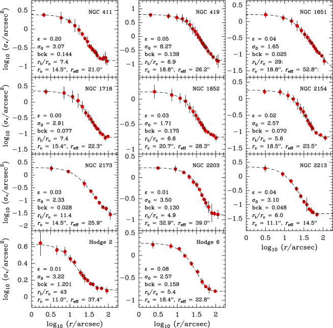
Figure 1.— Radial surface number density profiles of the star clusters in our sample that were not analyzed before in Goudfrooij et al. (2009) or Goudfrooij et al. (2011a). The points represent observed (completeness-corrected) values, while dashed lines represent the best-fit King (1962) models whose parameters are shown in the legends, along with the names and ellipticities of the clusters.

Cluster masses are determined from the $V$-band magnitudes listed in Table 1. Using the measurement aperture size of those integrated-light magnitudes along with the best-fit King model parameters of each cluster, we first determine the fraction of total cluster light encompassed by the measurement aperture. This is done using a routine that interpolates within points of a fine radial grid while calculating the integral of the King (1962) function. After correcting the integrated-light $V$ magnitudes for the missing cluster light beyond the measurement aperture, total cluster masses are calculated from the values of $A_{V}$, $(m-M)_{0}$, [$Z$/H], and age listed in Table 1. This process involves interpolation between the ${\cal{M}}/L_{V}$ values listed in the SSP models of Bruzual & Charlot (2003), assuming a Salpeter (1955) initial mass function (IMF). The latter models were recently found to provide the best fit (among popular SSP models) to observed integrated-light photometry of LMC clusters with ages and metallicities measured from CMDs and spectroscopy of individual RGB stars in the 1 – 2 Gyr age range (Pessev et al., 2008).

4.2. Dynamical Evolution of the Star Clusters

We perform the dynamical evolution calculations described in Goudfrooij et al. (2011b) for all clusters in our sample. Briefly, this involves the evaluation of the evolution of cluster mass and effective radius for model clusters with and without initial mass segregation. All calculations cover an age range of 10 Myr to 13 Gyr, and take into account the effects of stellar evolution mass loss and internal two-body relaxation. For the case of model clusters with initial mass segregation, we adopt the results of the simulation called SG-R1 in D’Ercole et al. (2008), which involves a tidally limited model cluster that features a level of initial mass segregation of $r_{\rm e}/r_{{\rm e,}\,>1}=1.5$, where $r_{{\rm e,}\,>1}$ is the effective radius of the cluster for stars with ${\cal{M}}>1\,M_{\odot}$. The primary reason why this simulation was selected for the purposes of the current paper is that it yields a number ratio of first-to-second-generation stars (hereafter called FG:SG ratio) of $\approx$ 1:2 at an age of $\sim$ 1.5 Gyr, which is similar to that seen in the clusters in our sample with the largest core radii (e.g., NGC 419, NGC 1751, NGC 1783, NGC 1806, NGC 1846), which likely had the highest levels of initial mass segregation (Mackey et al., 2008b, see discussion in § 5.4 below). In contrast, the simulations of clusters that do not fill their Roche lobes by D’Ercole et al. (2008, e.g., their SG-R05, SG-R06, and SG-R075 models) have FG:SG ratios $\sim$ 5:1 – 3:1, which are inconsistent with the observations of the aforementioned clusters in our sample.

We note that several young clusters in the Milky Way and the Magellanic Clouds exhibit high levels of mass segregation which is most likely primordial in nature (e.g., Hillenbrand & Hartmann, 1998; Fischer et al., 1998; Sirianni et al., 2000, 2001; de Grijs et al., 2002; Mackey et al., 2008b). For some clusters the level of mass segregation is actually higher than that in the SG-R1 model mentioned above (e.g., R136, in which stars with ${\cal{M}}>3\;M_{\odot}$ are a factor $\sim$ 4 more centrally concentrated than stars with ${\cal{M}}<3\;M_{\odot}$, see Sirianni et al. 2000). For clusters with such high levels of initial mass segregation, the simulations of Vesperini et al. (2009) suggest that they may dissolve in a few Gyr if they fill their Roche lobe. Hence, one should not discard the possibility that some of the intermediate-age clusters in the Magellanic Clouds may actually dissolve before reaching “old age”. This fate may be most likely for the intermediate-age clusters with the largest core radii and/or the lowest current masses (see discussion in § 5.5 below).

To estimate the systematic uncertainty of our mass loss rates for the case of clusters with initial mass segregation, we repeat our calculations for the case of the SG-C10 simulation of D’Ercole et al. (2008), which yields a FG:SG ratio at an age of 1.5 Gyr that is somewhat smaller than the SG-R1 simulation, while still being broadly consistent with the FG:SG ratios observed in the clusters in our sample with the largest core radii. A comparison of the two calculations indicates that the systematic uncertainty of our mass loss rates for the case of initial mass segregation is of order 30%.

4.3. Escape Velocities

Escape velocities are determined for every cluster by assuming a single-mass King model with a radius-independent ${\cal{M}}/L$ ratio as calculated above from the clusters’ best-fit age and [$Z$/H] values. Escape velocities are calculated from the reduced gravitational potential, $v_{\rm esc}(r,t)=(2\Phi_{\rm tid}(t)-2\Phi(r,t))^{1/2}$, at the core radius. Here $\Phi_{\rm tid}$ is the potential at the tidal (truncation) radius of the cluster. We choose to calculate escape velocities at the cluster’s core radius in view of the prediction of the “in situ” scenario, i.e., that the second-generation stars are formed in the innermost regions of the cluster (e.g., D’Ercole et al., 2008). Note that this represents a change relative to the escape velocities in Goudfrooij et al. (2011b), which were calculated at the effective radius. For reference, the ratio between the two escape velocities can be approximated by $v_{{\rm esc},\,r_{c}}/v_{{\rm esc},\,r_{e}}=1.1075+0.4548\,\log c-0.4156\,(\log c)^{2}+0.1772\,(\log c)^{3}$ where $c=r_{\rm t}/r_{\rm c}$ is the King concentration parameter. For King models with $5<c<130$, this approximation is accurate to within $\approx$ 3% rms.

For convenience, we define ${\cal{M}}_{\rm cl,7}\equiv{\cal{M}}_{\rm cl}\,(t=10^{7}{\rm yr})$ and $v_{\rm esc,7}(r)\equiv v_{\rm esc}\,(r,t=10^{7}{\rm yr})$ hereinafter, and refer to them as “early cluster mass” and “early escape velocity”, respectively. Masses and escape velocities of the clusters in our full sample are listed in Table 3 (at the end of this manuscript), both for the current ages and for an age of 10 Myr.

5. Pseudo-Age Distributions

5.1. Methodology

“Pseudo-age” distributions of the clusters in our sample are compiled following the steps described in Sect. 6.1 in Goudfrooij et al. (2011b). We construct a parallelogram in the region of the MSTO where the split between isochrones of different ages is evident and where the influence of unresolved binary stars is only minor (see § 5.2 below and Figs. 2 – 4), just below the ‘hook’ in the isochrone where core contraction occurs. One axis of the parallelogram is approximately parallel to the isochrones and the other axis approximately perpendicular to the isochrones. The magnitudes and colors of stars in the parallelogram are then transformed into the coordinate frame defined by the two axes of the parallelogram, after which we consider the distribution of stars in the coordinate perpendicular to the isochrones. The latter coordinate is translated to age by repeating the same procedure for the isochrone tables for an age range that covers the observed extent of the MSTO region of the cluster in question (using the same values of [Z/H], $(m\!-\!M)_{0}$ and $A_{V}$), and conducting a polynomial least-squares fit between age and the coordinate perpendicular to the isochrones.

The observed “pseudo-age” distributions of the clusters are compared to the distributions that would be expected in case the clusters are true SSPs (including unresolved binary stars) by conducting Monte-Carlo simulations as described below.

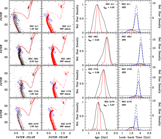
Figure 2.— Left panels: F475W versus F475W $-$ F814W CMDs of 4 star clusters in our sample with new WFC3 observations. Magnitudes are in the Vega-based system. Cluster names and ages are mentioned in the legends. Black dots represent stars within the clusters’ core radius. Magenta dots represent stars within “background regions” far away from the cluster center, with the same total area as the area within the core radius. The blue parallelogram depicts the region from which pseudo-age distributions were derived (see § 5.1). Second column of panels: F475W versus F475W $-$ F814W CMDs of the simulated star clusters (see § 5.2). The blue parallelogram from the left panels is included for comparison purposes. Third column of panels: Pseudo-age distributions of the star clusters (black lines) and of the associated SSP simulations (red lines). The best-fit binary fractions determined during the simulations are reported below the cluster names in the legend. Right panels: Estimates of star formation histories (SFHs) of the star clusters. The black and red lines are the same as in the third row of panels. The dashed lines indicate the SFHs of the clusters according to the SG-R1 model of D’Ercole et al. (2008). The solid blue lines indicate the clusters’ SFHs according to an estimated level of initial mass segregation for each cluster. The amplitudes of the SFHs are relative to the maximum star density reached in the pseudo-age distributions of the respective clusters. See § 5.4 for details.

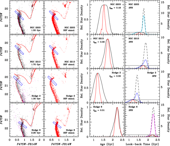
Figure 3.— Same as Figure 2, but now for 4 other star clusters with new WFC3 observations. The SFHs of NGC 2203 and Hodge 6 are plotted with cyan and magenta lines, respectively, for reasons discussed in § 5.4 (below equation 1).

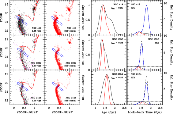
Figure 4.— Same as Figure 2, but now F555W versus F555W $-$ F814W CMDs for 3 other star clusters in our sample using ACS observations from the HST archive.

5.2. Monte Carlo Simulations

We simulate cluster CMDs of SSPs by populating the best-fit Marigo et al. (2008) isochrones (cf. § 3) with stars randomly drawn from a Salpeter IMF between the minimum and maximum stellar masses in the isochrone. The total number of stars in each simulation is normalized to the number of cluster stars on the CMD brighter than the 50% completeness limit. We add unresolved binary companions to a fraction (see below) of the stars, using a flat primary-to-secondary mass ratio distribution. Finally, we add random photometric errors to the simulated stars using the actual distribution of photometric uncertainties established during the artificial star tests.

We use the width of the upper main sequence, i.e. the part brighter than the turn-off of the field stellar population and fainter than the MSTO region of the clusters, to determine the binary star fraction in our sample clusters. The latter are mentioned on the right panels of Figs. 2 – 4. We estimate the internal systematic uncertainty of the binary fraction as $\pm 5\%$. For the purposes of this work the results don’t change significantly within $\sim\!10\%$ of the binary fraction.

The pseudo-age distributions of the clusters and their SSP simulations are depicted in Figs. 2 – 4. The left column of panels show the observed CMDs, the best-fit isochrone (whose properties are listed in Table 1), and the parallelogram mentioned in § 5.1 above (the latter in blue), the second column of panels show the simulated CMDs along with that same parallelogram, and the third column of panels show the pseudo-age distributions. The latter were calculated using the non-parametric Epanechnikov-kernel probability density function (Silverman, 1986), which avoids biases that can arise if fixed bin widths are used. In the case of the observed CMDs, this was done both for stars within the King core radius and for a “background region” far away from the cluster center. The intrinsic probability density function of the pseudo-age distribution of the clusters was then derived by statistical subtraction of the background regions. Stars in these background regions are plotted on the left panels of Figs. 2 – 4 as magenta dots. In the case of the simulated CMDs, the pseudo-age distributions are measured on the average of 10 Monte Carlo realizations.

5.3. Fraction of Clusters with eMSTOs in our Sample

As can be appreciated from the third column of panels of Figs. 2 – 4, the pseudo-age distributions of all but one clusters in our sample are significantly wider than that of their respective SSP simulations. This includes the case of NGC 2173, for which previous studies using ground-based data rendered the presence of an eMSTO uncertain (see Bertelli et al. 2003 versus Keller et al. 2012). We postulate that the effect of crowding on ground-based imaging in the inner regions of many star clusters at the distances of the Magellanic Clouds causes significant systematic photometric uncertainties that are largely absent in HST photometry.

The one cluster without clear evidence for an eMSTO is Hodge 6, for which the empirical pseudo-age distribution is only marginally wider than that of its SSP simulation. This is likely due at least in part to it being the oldest cluster in our sample (age = 2.25 Gyr). Since the width of pseudo-age distributions of simulated SSPs in Myr scales approximately with the logarithm of the clusters’ age (Goudfrooij et al., 2011a; Keller et al., 2011), the ability to detect a given age spread is age dependent, becoming harder for older clusters.

5.4. Relation to Star Formation Histories

We emphasize that the observed pseudo-age distributions shown in the third row of panels in Figs. 2 – 4 do not reflect the clusters’ star formation histories (SFHs) in case of clusters with non-negligible levels of initial mass segregation. This is due to the strong “impulsive” loss of stars taking place after the massive stars in the inner regions of mass-segregated clusters reach their end of life, which causes the cluster to expand beyond its tidal radius, thereby stripping its outer layers (e.g., Vesperini et al., 2009). In the context of the “in situ” scenario, this loss would mainly occur for the first generation of stars, as the second generation is formed in the innermost regions of the cluster after the impulsive loss of first-generation stars has finished (D’Ercole et al., 2008).

To estimate SFHs from the observed pseudo-age distributions of these star clusters in the context of the “in situ” scenario, one needs to consider (i) the evolution of the number of first– and second-generation stars from the clusters’ birth to the current epoch, and (ii) the age resolution element of the pseudo-age distributions, i.e., the shape of the function that describes a SSP in the pseudo-age distributions. For the latter, we use a gaussian with a FWHM equal to that of the pseudo-age distribution of the SSP simulation of the cluster in question (i.e., the red curves in the third column of panels in Figs. 2 – 4).

To evaluate consideration (i) above for the case of initially mass-segregated clusters, we again adopt the results of the simulation called SG-R1 in D’Ercole et al. (2008, see their Fig. 15). However, rather than using a given fixed level of initial mass segregation for every cluster, we consider it likely that this level varied among clusters. This implies that the (time-dependent) number ratio of initial-to-current first-generation stars (defined here as ${\it NR}_{\rm FG}(t)\equiv N_{\rm FG}^{\rm init}/N_{\rm FG}(t)$) also varies among clusters. To estimate a plausible value of ${\it NR}_{\rm FG}(t)$ for each cluster, we use results of the study by Mackey et al. (2008b) who showed that the maximum core radius seen among a large sample of Magellanic Cloud star clusters increases approximately linearly with log (age) up to an age of about 1.5 Gyr, namely from $\simeq$ 2.0 pc at $\simeq$ 10 Myr to $\simeq$ 5.5 pc at $\simeq$ 1.5 Gyr. In contrast, the minimum core radius is about 1.5 pc throughout the age range 10 Myr – 2 Gyr. N-body modeling by Mackey et al. (2008b) showed that this behavior is consistent with the adiabatic expansion of the cluster core in clusters with varying levels of initial mass segregation, in the sense that clusters with the highest level of initial mass segregation experience the strongest core expansion.

Another result of the simulations by Mackey et al. (2008b) that is relevant to the current discussion is the impact of the retention of stellar black holes (BHs) to the evolution of the clusters’ core radii. As shown in their Figs. 5, 15, and 21, simulated clusters that are able to retain the BHs formed earlier by stellar evolution of the massive stars experience a continuation of core expansion at ages $\gtrsim$ 1 Gyr, due to superelastic collisions between BH binaries and other BHs in the central regions. In contrast, clusters that do not retain stellar BHs start a slow core contraction process at an age of $\sim$ 1 Gyr due to two-body relaxation. While the currently available data do not allow direct constraints on the BH retention fraction of the clusters in our sample, the results of the simulations by Mackey et al. (2008b) do imply that the large core radii of clusters with ages in the approximate range of 1 – 2 Gyr and core radii $r_{\rm c}\gtrsim 5.5$ pc do not necessarily indicate extraordinarily high levels of initial mass segregation, even though their levels of initial mass segregation are likely still higher than for clusters in that age range that have $r_{\rm c}\lesssim 3.5$ pc. A more complex degeneracy is present for clusters in the age range of $\sim$ 2 – 3 Gyr with $3.5\lesssim r_{\rm c}/{\rm pc}\lesssim 5.5$. Such clusters can be produced by simulations of clusters without initial mass segregation that do retain their BHs just as well as by simulations with significant levels of initial mass segregation that do not retain their BHs (see Fig. 5 in Mackey et al. 2008b).

With this in mind, we tentatively assign values of ${\it NR}_{\rm FG}(t)$ to each cluster in the following way. For clusters with $r_{\rm c}\leq 5.5$ pc and an age in the range 1 – 2 Gyr, we assume that the (current) size of the core radius reflects the level of initial mass segregation of the cluster and we set the “plausible” value of ${\it NR}_{\rm FG}(t)$ as follows:

$${\it NR}_{\rm FG}^{p}(t)\equiv{\rm max}\left(1,{\it NR}_{\rm FG}^{\rm seg}(t)\;\times\left(\frac{r_{\rm c}-1.5}{5.5-1.5}\right)\right)\mbox{.}$$ (1)

where ${\it NR}_{\rm FG}^{\rm seg}(t)$ is the number ratio of initial-to-current first-generation stars calculated for the case of the SG-R1 model of D’Ercole et al. (2008). For clusters in our sample with $r_{\rm c}>5.5$ pc and ages $>$ 1.5 Gyr, we hypothesize that the core radius may have increased due in part to dynamical effects related to the presence of stellar-mass black holes in the central regions. This makes it hard to relate the current core radius to a particular level of initial mass segregation, even though this level is most likely still substantial. Hence we simply estimate ${\it NR}_{\rm FG}^{p}(t)\equiv{\it NR}_{\rm FG}^{\rm seg}(t)\times 2/3$ for such clusters. Recognizing that the values of ${\it NR}_{\rm FG}^{p}(t)$ for these clusters are inherently more uncertain than for those with $r_{\rm c}\leq 5.5$ pc, we plot the resulting SFHs with cyan lines in Figs. 2 – 4 (right-hand panels). Finally, SFHs of clusters with ages $\geq 2$ Gyr and $3.5\leq r_{\rm c}/{\rm pc}<5.5$ are assigned magenta lines in Figs. 2 – 4.

The SFH of a given cluster is then estimated by applying the inverse evolution of the number of first-generation stars (i.e., the multiplicative factor ${\it NR}_{\rm FG}^{p}(t)$) to the “oldest” resolution element of the pseudo-age distribution, i.e., a resolution element whose wing on the right-hand (“old”) side lines up with the “oldest” non-zero part of the cluster’s pseudo-age distribution. In contrast, the inverse evolution of the number of second-generation stars is applied to the full pseudo-age distribution. The resulting SFHs are shown in the right-hand panels of Figs. 2 – 4. For the estimated levels of initial mass segregation of the clusters in our sample, our results indicate that the SFR of the first generation dominated that of the second generation by factors between about 3 and 10.

5.5. Relations Between MSTO Width and Early Dynamical Properties

To quantify the differences between the pseudo-age distributions of the cluster data and those of their SSP simulations in terms of intrinsic MSTO widths of the clusters, we measure the widths of the two sets of distributions at 20% and 50% of their maximum values (hereafter called W20 and FWHM, respectively), using quadratic interpolation. The intrinsic pseudo-age ranges of the clusters are then estimated by subtracting the simulation widths in quadrature:

$${\it W20}_{\rm MSTO} = ({\it W20}_{\rm obs}^{2}-{\it W20}_{\rm SSP}^{2})^{1/2}$$

$${\it FWHM}_{\rm MSTO} = ({\it FWHM}_{\rm obs}^{2}-{\it FWHM}_{\rm SSP}^{2})^{1/2}$$ (2)

where the “obs” subscript indicates measurements on the observed CMD and the “SSP” subscript indicates measurements on the simulated CMD for a SSP. Given the insignificant difference between the width of the MSTO of Hodge 6 and that of its SSP simulations, we designate its resulting values for ${\it FWHM}_{\rm MSTO}$ and ${\it W20}_{\rm MSTO}$ as upper limits. The same is done for the lower-mass LMC clusters NGC 1795 and IC 2146 (with ages of 1.4 and 1.9 Gyr, respectively) for which Correnti et al. (2014) finds their MSTO widths to be consistent with those of their SSP simulations to within the uncertainties (see also Milone et al., 2009), even though two other intermediate-age LMC clusters with similarly low masses (but different structural parameters) do exhibit eMSTOs.

5.5.1 A Correlation Between MSTO Width and Early Cluster Mass

We plot ${\it W20}_{\rm MSTO}$ and ${\it FWHM}_{\rm MSTO}$ versus $\cal{M}_{\rm cl}$ at the current age in Figures 5a and 5b, respectively. Note that the width of the MSTO region seems to correlate with the cluster’s current mass. To quantify this impression, we perform statistical tests for the probability of a correlation in the presence of upper limits, namely the Cox Proportional Hazard Model test and the generalized Kendall’s $\tau$ test (see Feigelson & Nelson 1985). The results are listed in Table 4. The probabilities of the absence of a correlation are small: $p<1.3$%. However, we remind the reader that the clusters plotted here have different ages and radii, and hence likely underwent different amounts of mass loss since their births. This complicates a direct interpretation of this correlation in terms of constraining formation scenarios. To estimate the nature of this relation at a cluster age of 10 Myr, we therefore also plot ${\it W20}_{\rm MSTO}$ and ${\it FWHM}_{\rm MSTO}$ against $\cal{M}_{\rm cl,\,7}$ in Figs. 5c and 5d, respectively. In view of the uncertainty of assigning initial levels of mass segregation to individual clusters, we consider a range of possible $\cal{M}_{\rm cl,\,7}$ values for each cluster, shown by dashed horizontal lines in Figs. 5c and 5d. The minimum and maximum values of $\cal{M}_{\rm cl,\,7}$ for each cluster are the values resulting from the calculations without and with initial mass segregation, respectively. These values will be called $\cal{M}_{\rm cl,\,7}^{\rm noseg}$ and $\cal{M}_{\rm cl,\,7}^{\rm seg}$ hereinafter.

As seen in Figs. 5c and 5d, the range of possible $\cal{M}_{\rm cl,\,7}$ values for a given cluster can be significant. This is especially so for the older clusters in our sample, owing to the longer span of time during which the cluster has experienced mass loss. To estimate a plausible value of $\cal{M}_{\rm esc,\,7}$ for each cluster, we follow the arguments based on the results of the Mackey et al. (2008b) study described in the previous section. For clusters with $r_{\rm c}\leq 5.5$ pc and an age $\leq$ 2 Gyr, we thus set the “plausible” value of $\cal{M}_{\rm cl,\,7}$ as follows:

$${\cal{M}}_{\rm esc,\,7}^{p}\equiv{\cal{M}}_{\rm cl,\,7}^{\rm noseg}+({\cal{M}}_{\rm cl,\,7}^{\rm seg}-{\cal{M}}_{\rm cl,\,7}^{\rm noseg})\;\times\left(\frac{r_{\rm c}-1.5}{5.5-1.5}\right)\mbox{.}$$ (3)

These values of ${\cal{M}}_{\rm cl,\,7}^{p}$ are shown by large green symbols in Figs. 5c and 5d. For clusters in our sample with $r_{\rm c}>5.5$ pc and ages $>$ 1.5 Gyr, we estimate ${\cal{M}}_{\rm cl,\,7}^{p}\equiv({\cal{M}}_{\rm cl,\,7}^{\rm noseg}+{\cal{M}}_{\rm cl,\,7}^{\rm seg}\times 2)/3$ and we plot them with large red symbols in Figs. 5c and 5d. Finally, ${\cal{M}}_{\rm cl,\,7}^{p}$ values of clusters with ages $\geq 2$ Gyr and $3.5\leq r_{\rm c}/{\rm pc}<5.5$ are assigned large magenta symbols in Figs. 5c and 5d. We also included the results for the two low-mass LMC clusters NGC 1795 and IC 2146 studied by Correnti et al. (2014).

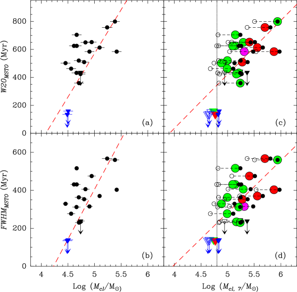
Figure 5.— Panel (a): W20_MSTO versus $\cal{M}_{\rm cl}$, the current cluster mass. Upper limits to W20_MSTO are indicated by triangles and downward arrows. Black symbols represent clusters in our sample, while dark blue symbols represent NGC 1795 and IC 2146, two low-mass clusters from the Milone et al. (2009) sample. The red dashed line represents a linear regression fit to the data using the Buckley-James method which takes upper limits into account (see Feigelson & Nelson, 1985). Panel (b): Similar to panel (a), but now FWHM_MSTO versus $\cal{M}_{\rm cl}$. Panel (c): Similar to panel (a), but now W20_MSTO versus $\cal{M}_{\rm cl,\,7}$, the cluster mass calculated for an age of 10 Myr (see § 4.2). Small open and small filled symbols indicate values of $\cal{M}_{\rm cl,\,7}$ for models without and with initial mass segregation, respectively. Large symbols in green, red, or magenta indicate educated guesses for the actual values of $\cal{M}_{\rm cl,\,7}$ for the clusters (see discussion in § 5.5 for the meaning of the colors). The dotted line indicates log($\cal{M}_{\rm cl,\,7}$) = 4.8, which seems to represent the approximate early cluster mass above which clusters seem to be able to host an eMSTO. The red dashed line represents a linear regression fit to the large green, red, and magenta symbols. Panel (d): Similar to panel (c), but now FWHM_MSTO versus $\cal{M}_{\rm cl,\,7}$. See discussion in § 5.5.1.

The distribution of the “large” symbols in Figs. 5c and 5d again reveals a correlation between the width of the MSTO region and the early cluster mass. Results of correlation tests are listed in Table 4. The correlations between MSTO width and early cluster mass are significant, with $p$ values that are $\simeq$ 50% smaller than those for the relations of the FWHM widths with the current cluster masses.

Comparing the early masses of the clusters that exhibit eMSTOs with those that do not, our results indicate that the “critical mass” needed for the creation of an eMSTO is around log(${\cal{M}}_{\rm cl,\,7})\approx 4.8$, indicated by a dotted line in Figs. 5c and 5d. This contrasts with the predictions of the “in situ” star formation model of Conroy & Spergel (2011) in terms of the minimum mass required for clusters to be able to accrete pristine gas from the surrounding ISM in the LMC environment, which they estimated to be $\approx 10^{4}\;M_{\odot}$. In other words, our results indicate that this minimum mass may be a factor $\approx 6-8$ higher than that estimated by Conroy & Spergel (2011). However, the data in Fig. 5 do not reveal an obvious minimum mass threshold in this context, and some young star clusters in the LMC without signs of an eMSTO are more massive than this (e.g., NGC 1856 and NGC 1866: ${\cal{M}}_{\rm cl}\sim 10^{5}\;M_{\odot}$, Bastian & Silva-Villa 2013). This may indicate that other properties (in addition to the early cluster mass) are relevant in terms of the ability of star clusters to accrete gas from their surroundings (e.g., the cluster’s velocity relative to that of the surrounding ISM, cf. Conroy & Spergel 2011, and the actual local distribution of ISM at the time).

5.5.2 A Correlation Between MSTO Width and Early Escape Velocity

We plot ${\it W20}_{\rm MSTO}$ and ${\it FWHM}_{\rm MSTO}$ versus $v_{\rm esc}$ at the current age in Figures 6a and 6b, respectively. Similar to the correlation with cluster mass shown in Figures 5, the width of the MSTO region correlates with the cluster’s current escape velocity. In this case, the probabilities of the absence of a correlation are $p\lesssim 0.3$% (see Table 4), which is significantly lower than for the relation between MSTO width versus cluster mass.

To estimate the nature of the relation of the MSTO width with escape velocity at a cluster age of 10 Myr, we plot ${\it W20}_{\rm MSTO}$ and ${\it FWHM}_{\rm MSTO}$ against $v_{\rm esc,\,7}$ in Figs. 6c and 6d, respectively. “Plausible” values of $v_{\rm esc,\,7}$ were determined using the assignments of levels of initial mass segregation and its associated scaling relations described above in § 5.5.1.

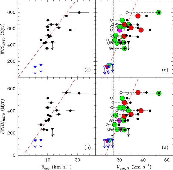
Figure 6.— Panel (a): W20_MSTO versus $v_{\rm esc}$, the current escape velocity at the core radius. Symbols are the same as for Figure 5a. The red dashed line represents a formal linear inverse-variance weighted fit to the data. Panel (b): Similar to panel (a), but now FWHM_MSTO versus $v_{\rm esc}$. Panel (c): Similar to panel (a), but now W20_MSTO versus $v_{\rm esc,\,7}$, the escape velocity at the core radius calculated for an age of 10 Myr (see §§ 4.2 and 4.3). Symbols are the same as for Figure 5c. The dotted line indicates $v_{\rm esc,\,7}$ = 15 km s^-1. The red dashed line represents a formal linear fit to the large green, red, and magenta symbols. Panel (d): Similar to panel (c), but now FWHM_MSTO versus $v_{\rm esc,\,7}$. See discussion in § 5.5.2.

Table 4Results of correlation tests.

Relation	$p_{\rm cox}$	$\tau$	$Z$	$p_{\tau}$
(1)	(2)	(3)	(4)	(5)
W20MSTO vs. log(${\cal{M}}_{\rm cl}$)	0.0006	0.8737	2.712	0.0067
FWHMMSTO vs. log(${\cal{M}}_{\rm cl}$)	0.0006	0.8000	2.479	0.0132
W20MSTO vs. log(${\cal{M}}_{\rm cl,\,7}^{p}$)	0.0013	0.8947	2.778	0.0055
FWHMMSTO vs. log(${\cal{M}}_{\rm cl,\,7}^{p}$)	0.0012	0.8211	2.544	0.0110
W20MSTO vs. $v_{\rm esc}$	0.0002	0.9263	2.877	0.0040
FWHMMSTO vs. $v_{\rm esc}$	0.0002	0.9684	3.001	0.0027
W20MSTO vs. $v_{\rm esc,\,7}^{p}$	0.0001	1.0421	3.235	0.0012
FWHMMSTO vs. $v_{\rm esc,\,7}^{p}$	0.0001	0.9789	3.035	0.0024

The distribution of the “large” symbols in Figures 6c and 6d again shows that FWHM_MSTO (or W20_MSTO) is correlated with $v_{\rm esc,\,7}^{p}$ in that clusters with larger early escape velocities have wider MSTO regions. A glance at Table 4 shows that these correlations are highly significant, with $p$-values that are about half of those for the relations of the MSTO widths with the current escape velocities. The $p$-values for the relation between MSTO width and escape velocity are also significantly lower than those for the relation between MSTO width and cluster mass, suggesting a more causal correlation for the former. Finally, Figs. 6c and 6d suggest that eMSTOs occur only in clusters with early escape velocities $v_{\rm esc,\,7}\gtrsim$ 12 – 15 km s^-1.

6. Discussion

We review how our results compare with recent predictions of the “stellar rotation” and the “in situ star formation” scenarios below. We also compare our results with relevant findings in the recent literature, and comment on the feasibility of other scenarios to explain the eMSTO phenomenon in the light of our results. Finally, we discuss our results in the context of the currently available data on light-element abundance variations within the clusters in our sample.

6.1. Comparison with Stellar Rotation Scenario

6.1.1 MSTO Widths

To compare the MSTO widths with predictions of the stellar rotation scenario, we use results from the recent study of Yang et al. (2013) who calculated evolutionary tracks of non-rotating and rotating stars for three different initial stellar rotation periods (approximately 0.2, 0.3, and 0.4 times the Keplerian rotation rate of ZAMS stars), and for two different mixing efficiencies (“normal”, $f_{c}$ = 0.03, and “enhanced”, $f_{c}$ = 0.20). From the isochrones built from these tracks, they calculated the widths of the MSTO region caused by stellar rotation as a function of cluster age and translated them to age spreads (in Myr). In the context of the pseudo-age distributions derived for our clusters in Section 5.2, the age spreads due to rotation calculated by Yang et al. (2013) are equivalent to the full widths of the age distribution (W. Yang, 2014, private communication). Hence we compare their age spreads with our W20 values. Using the results shown in Fig. 8 of Yang et al. (2013), we assemble the ranges encompassed by their age spreads as a function of age for the two different mixing efficiencies. These ranges are shown as grey regions delimited by solid and dashed curves in Figure 7, which shows W20_MSTO as function of age for the clusters in our sample.

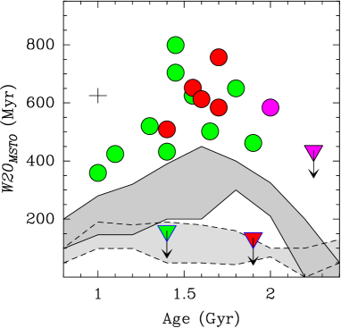
Figure 7.— W20_MSTO versus cluster age. Symbols are the same as the “large” symbols in Fig. 6. The grey areas delimited by solid and dashed lines represent the ranges of MSTO width as function of age due to stellar rotation effects found by Yang et al. (2013) for mixing efficiencies $f_{c}$ = 0.03 and 0.20, respectively. See discussion in § 6.1.

Figure 7 reveals some interesting results. First of all, many clusters in our sample feature MSTO widths that are significantly larger than stellar rotation seems to be able to produce at their age according to the Yang et al. (2013) study. This result, along with the finding that W20_MSTO correlates with $v_{\rm esc,\,7}$, suggests strongly that the eMSTO phenomenon is at least partly due to “true” age effects. Second, stellar rotation at “normal” mixing efficiency seems to be able to produce age spreads that generally follow the lower envelope of the measured W20_MSTO values of the star clusters in our sample as a function of their age. This by itself could indicate that the MSTO broadening of these clusters could also be due in part to stellar rotation, for example if some clusters might host significant numbers of stars with rotation rates $>$ 0.4 times the Keplerian rate. However, the two clusters with ages in the 1 – 2 Gyr range that do not show any measurable amount of MSTO broadening (NGC 1795 and IC 2146) are inconsistent with this view, unless stellar rotation in such clusters (with low values of $v_{\rm esc,\,7}$) either occurs at much lower rotation velocities or at significantly higher mixing efficiency than in clusters with higher values of $v_{\rm esc,\,7}$.

In this context we note two reasons suggesting that stellar rotation rates should not be significantly different in those two low-mass clusters relative to the other clusters in our sample: (i) the absolute difference in $v_{\rm esc,\,7}$ between those two clusters and the lowest-mass clusters in our sample that do feature eMSTOs is not huge ($\approx$ 9 – 12 vs. 16 – 20 km s^-1). This difference is even smaller when considering their current masses or escape velocities (see Figs. 5 and 6). Hence, the onset of the widening of the MSTO seems more likely to be caused by a “minimum” threshold escape velocity (at early times) than by pure relative depths of the clusters’ potential wells (see also Correnti et al. 2014 and § 6.2 below). (ii) In a recent study of the Galactic open cluster Trumpler 20, the only star cluster in the age range of 1 – 2 Gyr for which stellar rotation velocities have been measured to date using high-resolution spectroscopy, Platais et al. (2012) found an approximately flat distribution of rotation velocities of MSTO stars in the range $180<V\sin i<0$ km s^-1. This implies a range of rotation rates very similar to that considered by the Yang et al. (2013) models, even though this is a loose cluster with very low escape velocity. Furthermore, Platais et al. (2012) found that the 50% fastest rotators in Trumpler 20 are actually marginally blueshifted on the CMD with respect to the slow rotators ($\delta(V-I)=-0.01$, see Platais et al. 2012). These findings are inconsistent with the predictions of Yang et al. (2013) for “normal” mixing efficiency, but they are marginally consistent with their predictions for high mixing efficiency (see Fig. 7). While it is not clear to us why the efficiency of rotational mixing in stars would be higher in clusters with lower potential well depths, this may be an avenue for future research. We also recognize that the study of the creation of theoretical stellar tracks and isochrones for rotating stars at various stages of stellar evolution, rotation rates, and ages is still in relatively early stages, and that our comparison with model predictions such as those of Yang et al. (2013) implicitly involves adopting the assumptions made by those models. Furthermore, no stellar rotation measurements have yet been undertaken in intermediate-age star clusters in the Magellanic Clouds. Hence, future findings in this context might affect our conclusions on the nature of eMSTOs. However, for now, the observations of Platais et al. (2012) are most consistent with the predictions of Girardi et al. (2011), i.e., that stellar models with rotation produce a marginal blueshift in the MSTO of star clusters with ages in the range 1 – 2 Gyr rather than a reddening as predicted by Bastian & de Mink (2009) and Yang et al. (2013).

6.1.2 Red Clump Morphologies

Focusing on the RC feature in the CMDs of the star clusters in our sample as a function of their (average) age, one can identify certain trends that are relevant to the nature of eMSTOs. Firstly, the RC feature can often be seen to extend to fainter magnitudes than the RC feature of the clusters’ respective SSP simulations. This is especially the case for the relatively massive clusters NGC 411, NGC 419, NGC 1852, and NGC 2203; hints of this effect also appear in NGC 2154, and NGC 2173. This “composite red clump” feature was already reported before in NGC 411, NGC 419, NGC 1751, NGC 1783, and NGC 1846 (Girardi et al., 2009, 2013; Rubele et al., 2010, 2013), and is thought to be due to the cluster hosting stars massive enough to avoid electron degeneracy settling in their H-exhausted cores when He ignites. The main part of the RC consists of less massive stars which did pass through electron degeneracy prior to He ignition (Girardi et al., 2009). This causes the brightness of RC stars to increase relatively rapidly with decreasing stellar mass in the narrow age range of $\simeq$ 1.00 – 1.35 Gyr, after which that increase slows down significantly due to the fact that all RC stars experienced electron degeneracy prior to He ignition. Interestingly, the composite RCs are seen in all clusters in our sample for which the pseudo-age distributions indicate the presence of a non-negligible number of stars in that age range, even though their best-fit age is always older than 1.35 Gyr.

This has an impact to the feasibility of the “stellar rotation” scenario in causing the eMSTOs for these clusters. In this scenario, stars with high rotation velocities have larger core masses at the end of the MS era than do non-rotating stars (e.g., Maeder & Meynet, 2000; Eggenberger et al., 2010; Yang et al., 2013). In this respect, fast rotators could in principle present the modest increase in the core mass necessary to ignite Helium before the settling of electron degeneracy, and hence cause the faint extension of the RC as well. However, the (small) fraction of RC stars in its faint extension scales with the fraction of MSTO stars at the youngest ages in these clusters, i.e., at ages in the 1.00 – 1.35 Gyr range, which are at the blue and bright end of the MSTO. This is illustrated in Figure 8. Figure 8a shows the CMD of NGC 2203 (as an example) along with three isochrones for ages 1.35, 1.60, and 1.85 Gyr. These isochrones coincide approximately with the upper left edge, the mean location, and the lower right edge of its eMSTO feature, respectively. The RC and AGB parts of the same isochrones are also shown on top of the RC of NGC 2203. The faint “secondary RC” feature (cf.  Girardi et al., 2009), which is shown as a yellow parallelogram, is then defined as the area in the CMD “below” the horizontal branch (HB) of the 1.35 Gyr isochrone; the tilt of the short side of the parallelogram equals that of the HB of the 1.35 Gyr isochrone. The “full RC” area is then approximated by extending the “secondary RC” area toward brighter magnitudes so as to also encompass the full HB of the “oldest” isochrone, allowing for suitable photometric errors. (This extension is shown as a light grey parallelogram in Fig. 8a.) We then evaluate the fraction of RC stars in the secondary RC, defined as $f_{\rm RC}(<1.35\;{\rm Gyr})\equiv N\mbox{(secondary RC)}/N\mbox{(full RC)}$. This fraction is plotted versus $f_{\rm MSTO}(<1.35\;{\rm Gyr})$, the fraction of stars in the pseudo-age distributions at ages $\leq$ 1.35 Gyr, in Figure 8b for all clusters whose pseudo-age distribution in Figs. 2 – 4 indicates the presence of a significant number of stars with ages $\leq$ 1.35 Gyr even though their average age is older. Note that even though the Poisson uncertainties are significant, the data indicate an approximate 1:1 relation between the fraction of RC stars in the faint extension and the fraction of MSTO stars in the part on the “upper left” side of the 1.35 Gyr isochrone. Note that the sense of this relation is consistent with that predicted in case the width of eMSTOs reflects a range in stellar ages, while it is contrary to the predictions of Bastian & de Mink (2009) and Yang et al. (2013) which were that high stellar rotation velocities cause stars to populate the lower right end of the MSTO at the ages of these clusters. This suggests that eMSTOs are indeed due mainly to a range of stellar ages rather than a range of stellar rotation velocities among MSTO stars. This result would benefit from confirmation by future isochrones of rotating stars that include the stages of stellar evolution past the Helium flash on the RGB as well as a relevant range of (initial) rotation velocities.

Secondly, we note that the composite RCs are not seen in eMSTO clusters for which the “pseudo-age” distribution does not indicate any significant number of stars with ages $\lesssim 1.35$ Gyr, such as NGC 1651, NGC 1718, and NGC 2213. This suggests that the composite RCs are not caused by interactive binaries as proposed by Li et al. (2012), since the effect of interactive binaries on the RC morphology is not expected to depend on age (in the age range 1 – 2 Gyr).

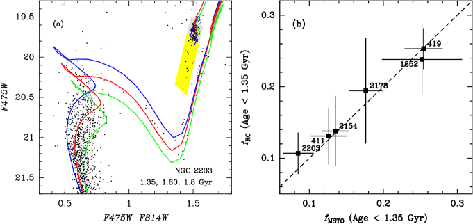
Figure 8.— Panel (a): CMD of stars within the core radius of NGC 2203, zooming in on the MSTO and RC regions. The blue, red, and green lines depict Marigo et al. (2008) isochrones with ages 1.35, 1.60, and 1.85 Gyr, respectively. The yellow parallelogram depicts the faint “secondary RC” region described in § 6.1, while the grey parallelogram depicts the part of the “full RC” region that is not part of the “secondary RC” region. Panel (b): the fraction of RC stars in the secondary RC plotted against the fraction of MSTO stars with ages $\leq$ 1.35 Gyr for clusters whose pseudo-age distribution shows a significant number of stars with ages $\leq$ 1.35 Gyr. The NGC numbers of the clusters are indicated next to their data points. The dashed line represents a 1:1 relation. See discussion in § 6.1.

6.2. Comparison with Extended Star Formation Scenario

In the context of the “in situ star formation” scenario, we first note that Figure 6 suggests that the onset of the eMSTO phenomenon occurs in the range $12\lesssim v_{\rm esc,\,7}\lesssim 15$ km s^-1. This range of early escape velocities agrees well with observed expansion velocities of the ejecta of the “polluter” stars thought to produce the Na-O anticorrelations among stars in globular clusters, as detailed below.

As to the case of IM-AGB stars, we turn our attention to OH/IR stars featuring the superwind phase on the upper AGB, which is thought to account for the bulk of mass loss of intermediate-mass stars (e.g., Vassiliadis & Wood, 1993). Radio observations of thermally pulsating OH/IR stars in our Galaxy show expansion velocities $v_{\rm exp}$ in the range 14 – 21 km s^-1, peaking at $\simeq$ 17 km s^-1 (e.g., Eder et al., 1988; te Lintel Hekkert et al., 1991). While expansion velocity measurements of OH/IR stars in the Magellanic Clouds are still scarce, 4 LMC OH/IR stars have been found to exhibit $v_{\rm exp}$ values that are $\sim$ 10 – 20% lower than the Galactic ones in a given OH luminosity class (Zijlstra et al., 1996). Taking this ratio at face value, this would translate into $v_{\rm exp}$ values in the range 12 – 18 km s^-1 for OH/IR stars in the LMC, peaking at $\simeq$ 15 km s^-1. This is exactly the range of early escape velocities within which we see the bifurcation between star clusters with versus without eMSTOs.

As to the case of massive stars, observations of nearby star forming regions suggest that most such stars are in binary systems (e.g., Sana et al., 2012). Hence we focus on the case of massive binary stars, for which imaging and spectroscopic observations have shown that the enriched material is mainly ejected in a disc or ring geometry with expansion speeds in the range 15 – 50 km s^-1 (e.g., Smith et al., 2002, 2007). Hence, the retention of mass-loss material from massive binary stars seems to require somewhat higher cluster escape velocities than that from IM-AGB stars. I.e., the rate of retention and accumulation of mass loss material from massive binary stars may scale with the clusters’ (early) escape velocities, and this material may not be available in significant quantities to eMSTO clusters with the lowest early escape velocities.

Next, we consider the hypothesis that the observed correlation between MSTO width and $v_{\rm esc,\,7}$ reflects the (evolving) depth of the potential well in the central regions of star clusters and its impact on the ability of a star cluster to (i) accrete an adequate amount of “pristine” gas from their surroundings, and/or (ii) retain chemically enriched material ejected by first-generation “polluter” stars, and make the resulting material available for second-generation star formation. To test this hypothesis, we use the cluster mass loss simulations described in § 4.2 which provide cluster mass and $v_{\rm esc}$ as function of time for the eMSTO clusters in our sample.

As indicated by Table 3, the masses of the clusters in our sample at an age of 10 Myr ranged between roughly $1\times 10^{5}\;M_{\odot}$ and $1\times 10^{6}$ $M_{\odot}$, for a reasonable range of levels of initial mass segregation. For such cluster masses, the calculations of Conroy & Spergel (2011, see their Figs. 2 – 3) predict that they were able to accrete $\approx$ 10 – 30% of their mass in “pristine” gas unless the velocity of the cluster relative to that of the surrounding ISM was $\gtrsim 600$ km s^-1. Such high relative velocities seem unlikely to occur in dwarf galaxies like the Magellanic Clouds (although it may well occur in the violent environment of merging massive galaxies). Even when taking into account the simplifying assumptions made in the study of Conroy & Spergel (2011), it therefore seems plausible that the eMSTO clusters in our sample were able to accrete significant amounts of pristine gas from their surroundings. To test part (ii) of the hypothesis mentioned above, we plot $v_{\rm esc}$ as function of time for the eMSTO clusters in our sample in Figures 9a – 9e in which each panel shows clusters with FWHM_MSTO values in a given range. The values of $v_{\rm esc}$ plotted in Figure 9 reflect the same levels of initial mass segregation as those used for the “large” symbols in Figure 6 (cf. § 5.5 above).

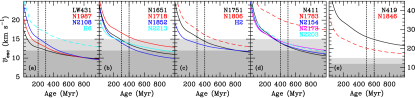
Figure 9.— $v_{\rm esc}$ versus time since cluster birth. Each curve depicts dynamical evolution simulations for a given cluster, identified in the legend at the top right in each panel. Dashed lines identify clusters for which the assignment of a particular level of initial mass segregation is relatively uncertain (i.e., clusters shown with red circles in Figs. 6 and 7). Light grey and dark grey areas indicate the ranges $v_{\rm esc}\leq 15$ km s^-1 and $v_{\rm esc}\leq 12$ km s^-1, respectively. Vertical dotted lines in each panel delineate the range in FWHM_MSTO encompassed by the clusters drawn in that panel. Note that panel (e) has a different vertical scale than panels (a) – (d). See discussion in § 6.2.

Figures 9a – 9d show that $v_{\rm esc}$ stays above 15 km s^-1 for ages up to 100 – 150 Myr for all eMSTO clusters in our sample. This is equivalent to the lifetime of stars of $\approx 4\;M_{\odot}$ (e.g., Marigo et al., 2008), and hence long enough for the slow winds of massive binary stars and IM-AGB stars of the first generation to produce significant amounts of “polluted” material out of which second-generation stars may be formed. This consistency between the escape velocity that seems to be required for retention of enriched mass-loss material and the escape velocities of eMSTO clusters at the time when the candidate polluter stars are present constitutes evidence in favor of the hypothesis stated above and hence of the “in situ star formation” scenario, in which the FWHM_MSTO values are a measure of the length of star formation activity.

Among the eMSTO clusters in our sample with $200\lesssim{\it FWHM}_{\it MSTO}/{\rm Myr}\lesssim 500$, $v_{\rm esc}$ crosses the range 12 – 15 km s^-1 at ages similar to those indicated by their values of FWHM_MSTO. As shown by Figure 9e, this behavior is not shared by the clusters with the largest values of FWHM_MSTO (i.e., in the approximate range 500 – 550 Myr) in that their escape velocities stay above 15 km s^-1 for periods longer than that indicated by their values of FWHM_MSTO. In the context of the “in situ star formation” scenario, this finding seems to indicate that the maximum length of the star formation era in the most massive star clusters is not set by the ability of a star cluster to retain chemically enriched material from polluter stars and/or to accrete gas from the surrounding ISM. Instead, we speculate that the observational limit of FWHM${}_{\it MSTO}\lesssim 550$ Myr may reflect the typical time when the collective rate of supernova (SN) events (i.e., “prompt” SN type Ia events by first-generation stars plus any SN II events by second-generation stars) starts to be high enough to sweep out the remaining gas in star clusters, thus ending the star formation era (see also Conroy & Spergel, 2011).

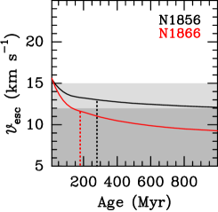
Figure 10.— Similar to Figure 9, but now for the young LMC clusters NGC 1856 and NGC 1866, using mass and radius data from McLaughlin & van der Marel (2005). Vertical dotted lines in this Figure indicate the current ages of the two clusters (280 Myr for NGC 1856 and 180 Myr for NGC 1866). See discussion in § 6.3.

6.3. Comparison with Recent Literature

Our results regarding the nature of eMSTO’s in intermediate-age star clusters generally favor the scenario in which eMSTO’s reflect a range of stellar ages in the cluster rather than a range of stellar rotation velocities among the MSTO stars. However, this conclusion seems to be at odds with a number of recent studies that showed that younger star clusters do not exhibit such age spreads. We discuss results of the latter studies in the context of the “in situ” scenario below. Recapitulating the latter scenario, if massive binary stars and/or rapidly rotating massive stars are the main source of gas out of which a second generation is to be formed, one would expect that material to become available for star formation after 5 – 20 Myr of a cluster’s life (if it is not swept out of the cluster by SN type II explosions of the massive stars). If instead AGB stars with $5\lesssim{\cal{M}}/M_{\odot}\lesssim 8$ are the main source of the enriched material, it would take $\sim$ 50 – 100 Myr to make it available for star formation. The actual era of second-generation star formation might not actually start until $\sim$ 100 – 150 Myr after the creation of the cluster, depending on the role of Lyman continuum photons from the massive stars of the first generation in prohibiting star formation through photodissociation of H₂ (Conroy & Spergel, 2011). This era could last an additional few 10⁸ yr depending on when the molecular gas reservoirs run out or when the rate of “prompt” SN type Ia events by first-generation stars becomes significant.

• The recent review of Portegies Zwart et al. (2010) presented known properties of young massive clusters (YMCs) in our Galaxy, including a number whose escape velocity is of order 12 – 15 km s^-1 (e.g., the Arches cluster, NGC 3603, RSGC01, RSGC03, and Westerlund 1). Perina et al. (2009) also presented a study of van den Bergh 0, a YMC with similar properties in M31. Such clusters would therefore be expected to be able to host extended star formation if the “in situ” scenario is correct. However, the CMDs of these YMCs do not show any signs of a significant spread in age. We suggest that these observations can be reconciled with the AGB version of the “in situ” scenario because the ages of all of these YMCs are $\lesssim 25$ Myr. At that time, the slow stellar winds from AGB stars have only just started, so that one would not yet expect to see any significant sign of second-generation stars.

• Larsen et al. (2011) presented CMDs of 6 massive YMCs ($10^{5}-10^{6}\;M_{\odot}$) in galaxies nearby enough to resolve the outskirts of the YMCs with HST photometry. The ages of these YMCs were found to be in the range 5 – 50 Myr. They find no evidence for significant age spreads, except for some of the older YMCs which show tentative evidence of age spreads of up to 30 Myr. Given (i) the time it takes for a SSP to produce significant amounts of gas from AGB mass loss and (ii) the fact that the second-generation stars are thought to form in the innermost regions of these clusters (e.g., $\simeq$ 85% of the second-generation stars in the D’Ercole et al. (2008) model are within 0.1 pc from the center, which region is overcrowded at the distances of these clusters), we believe these observations are not inconsistent with the “in situ” scenario.

• Bastian & Silva-Villa (2013) studied two relatively massive young LMC clusters (NGC 1856 and NGC 1866, with ages of 280 Myr and 180 Myr, respectively) and found no evidence for age spreads larger than about 20 – 35 Myr, which they interpreted as a suggestion that the eMSTO feature in intermediate-age clusters cannot be due to age spreads. To test this in the context of the dynamical properties of these two clusters, we follow Bastian & Silva-Villa (2013) by adopting the King model fits of those two clusters from the compilation of McLaughlin & van der Marel (2005, see Table 1 in ), and multiply their masses by a factor 1.6 since they were using the Chabrier IMF whereas we use the Salpeter IMF. After running the dynamical evolution models described in § 4.2 on those two clusters, we plot their resulting $v_{\rm esc}$ as function of time in Figure 10, whose setup is similar to that of Figure 9. In choosing the plausible value for $v_{\rm esc,\,7}$ for these clusters, we recognize that the observed range of core radii of Magellanic Cloud star clusters in the age range 200 – 300 Myr is approximately 1.5 – 4.5 pc (Mackey et al., 2008b) and hence we estimate $v_{\rm esc,\,7}^{p}$ as follows:

  $$v_{\rm esc,\,7}^{p}\equiv v_{\rm esc,\,7}^{\rm noseg}+(v_{\rm esc,\,7}^{\rm seg}-v_{\rm esc,\,7}^{\rm noseg})\;\times\left(\frac{r_{\rm c}-1.5}{4.5-1.5}\right)\mbox{.}$$ (4)

  Comparing the solid lines in Figure 10 with those in 9, one sees that $v_{\rm esc}$ for NGC 1856 and NGC 1866 never surpassed $\sim$ 15 km s^-1, whereas it did for all eMSTO clusters in our sample. However, the difference between the $v_{\rm esc,\,7}^{p}$ of NGC 1856 and NGC 1866 and that of the lowest-mass eMSTO clusters in our sample is relatively small (e.g., $v_{\rm esc,\,7}^{p}\simeq 17$ km s^-1 for LW431), indicating that the early escape velocity threshold that differentiates clusters with eMSTOs from those without might occur close to 15 km s^-1 when assuming a Salpeter IMF (see also Correnti et al., 2014). In that sense, the apparent absence of eMSTOs in NGC 1856 and NGC 1866 is not necessarily inconsistent with the “in situ star formation” scenario, although the margins seem to be small.

  In this context, we note that our King-model fits were done using completeness-corrected surface number densities, whereas McLaughlin & van der Marel (2005) used surface brightness data to derive structural parameters for NGC 1856 and NGC 1866. The latter method is sensitive to the presence of mass segregation in the sense that mass-segregated clusters will appear to have smaller radii (and hence higher escape velocities) when using surface brightness data than when using plain surface number densities. A study of the impact of this effect is currently underway using new HST data of NGC 1856 (M. Correnti et al., in preparation).

• Bastian et al. (2013b) studied the presence of ongoing star formation in a large sample of $\sim$ 130 YMCs, mainly using spectroscopy in the 4500 – 6000 Å wavelength region, by means of H$\beta$ and [O iii]$\lambda$5007 emission. Their sample of YMCs covered a significant range in best-fit ages (10 – 1000 Myr) and masses ($10^{4}-10^{8}\;M_{\odot}$), both derived from UBVRI photometry or the spectra themselves. Concentrating on YMCs that can significantly constrain the AGB version of the “in situ” scenario, we select YMCs from their sample that have: (i) ${\cal{M}}\gtrsim 10^{5}\;M_{\odot}$ (to create a high probability that $v_{\rm esc}\gtrsim 15$ km s^-1), (ii) ages in the range 100 – 300 Myr, and (iii) spectra that are shown in the literature (either in Bastian et al. (2013b) itself or in the references therein). This selection results in a sample of 21 YMCs. Inspection of their spectra reveals 4 clusters that seem to show hints of [O iii]$\lambda$5007 in emission and/or H$\beta$ emission filling in the deep absorption line (clusters M82-43.2, M82-98, NGC3921-S2, and NGC2997-376), i.e., $\lesssim$ 20% of the sample.

  This apparent lack of emission in a significant fraction of this subsample of YMCs studied by Bastian et al. (2013b) provides an important constraint to the “in situ” scenario, and therefore merits some discussion. One relevant consideration may be that the second-generation star formation is thought to occur in the innermost regions of the clusters (likely in a flattened structure), and extinction by the ISM in those regions may impact the detection of line emission. This possibility can be tested in the future by performing spectral observations at longer wavelengths and with emission lines that are intrinsically stronger than H$\beta$ and [O iii]$\lambda$5007 in H ii regions (e.g., H$\alpha$ and Br$\gamma$ from the ground, Pa$\alpha$ and Br$\alpha$ from space). Another consideration is that the duration of the line emission era in star-forming regions is only $\simeq$ 7 Myr, which is a very small fraction of the age spread indicated by the width of eMSTOs (or the time interval in which second-generation star formation is predicted to occur in the “in situ” scenario). It is not known whether this star formation would be occurring in a continuous fashion or perhaps in recurrent episodes. While the pseudo-age distributions of the clusters in our sample (i.e,. Figs. 2 – 4) do typically appear quite smooth, suggesting continuous star formation activity, we remind the reader that our time resolution element is similar to a gaussian with FWHM $\simeq$ 150 – 200 Myr, depending on the cluster age. We therefore cannot detect variations in the age distribution on time scales of several tens of Myr, leaving open the possibility of recurrent star formation activity. Finally, significant line emission in star-forming regions only occurs when there are enough O and B stars to ionize the gas, implying a dependence on the (a priori unknown) IMF of the second generation. The apparent lack of line emission in several YMCs at ages of $\sim$ 100 – 300 Myr might therefore still be consistent with the “in situ” scenario if second-generation stars are formed in regions where the IMF is such that O and B stars are relatively unlikely to form, and/or where the SFR is small relative to that of first-generation star-forming regions. We suggest that the likelihood of these possibilities be tested in the near future using new simulations as well as (IR) observations.

• Cabrera-Ziri et al. (2014) studied the SFH of the very massive young Cluster #1 in the merger remnant galaxy NGC 34, using a spectrum obtained earlier by Schweizer & Seitzer (2007). Using stellar population synthesis fitting, they find that the SFH of this cluster is consistent with a SSP of age 100 $\pm$ 30 Myr and rule out the presence of a second population that is younger than 70 Myr at a second-to-first-generation mass ratio of $\geq 0.1$. While these results provide important constraints on the presence of a second stellar generation in this cluster, it is not clear yet how much second-generation star formation one might expect at a cluster age of 100 Myr. According to Conroy & Spergel (2011), the density of Lyman continuum photons from massive stars of the first generation would likely still be high enough at this age to prohibit new star formation. Similar work for massive clusters at ages of 200 – 500 Myr should therefore yield more relevant constraints to the “in situ” scenario.

6.4. Comparison with Other Scenarios Involving a Range of Stellar Ages

The presence of a range of stellar ages within a star cluster does not necessarily imply that all cluster stars were formed “in situ” within the clusters. In this context, we briefly comment on the feasibility of two scenarios that involve an external origin of part of the stars in clusters while preserving the observed homogeneity in [Fe/H]: (1) the merger of two or more star clusters formed in a given giant molecular cloud (hereafter GMC), and (2) the merger of a (young) star cluster with a GMC.

As to possibility (1) above, a range of ages in clusters could be the result of merging of smaller clusters that were all formed by the collapse of a given GMC (in which multiple clusters were formed at different times). However, as explained by Goudfrooij et al. (2009), the observed age ranges of 200 – 500 Myr in eMSTO clusters are much larger than the observed age differences between binary or multiple clusters in the LMC (e.g., Dieball et al., 2002). Hence, it seems hard to form the eMSTO clusters by star formation within a given GMC in general, especially since the eMSTO phenomenon is very common among intermediate-age clusters in the Magellanic Clouds.

As to possibility (2), the simulations by Bekki & Mackey (2009) suggest that new episodes of star formation can be triggered by an interaction of a star cluster with a GMC, as long as the space velocity of the star cluster relative to that of the GMC is smaller than $\sim$ 2 times the internal velocity dispersion of the cluster. Several aspects of this scenario seem to be generally consistent with the observational evidence:

• As argued by Bekki & Mackey (2009), the typical time scale of a cluster-GMC merger can be of the same order as that indicated by the MSTO widths of eMSTO clusters if the (average) surface number density of GMCs in the LMC was a few times higher than it is now. This does not seem implausible: According to the SFH of the LMC published by Weisz et al. (2013), the LMC formed $\simeq$ 25% of its current stars over the last 2 Gyr. Using the current stellar and gas masses of the LMC given by van der Marel et al. (2002), this implies that the gas supply of the LMC decreased by $0.25\;{\cal{M}}_{\ast,\,{\rm LMC}}=7.6\times 10^{8}\;M_{\odot}$ over the last 2 Gyr. This is about 1.5 times its current gas mass, so that the LMC gas supply was a factor $\approx$ 2.5 larger when the clusters in our sample were created. Furthermore, the era of 1 – 2 Gyr ago in the Magellanic Clouds is thought to feature strong tidal interactions between the LMC and SMC, causing strong star (and star cluster) formation in the bar and NW arm of the LMC (e.g., Bekki et al., 2004; Diaz & Bekki, 2011; Besla et al., 2012; Rubele et al., 2012; Piatti, 2014), where many of the clusters in our sample are located. It thus seems reasonable to postulate that relatively high number densities of high-mass GMCs were relatively common at the time, allowing the formation of several massive star clusters and possibly creating a situation where the typical time scale of cluster-GMC mergers was similar to the age ranges indicated by FWHM_MSTO values of eMSTO clusters. Alternatively, the time scale of $\sim$ 100 – 500 Myr may reflect the typical life time of strong density waves during the tidal interactions between the LMC and SMC at the time, allowing strong cluster formation and cluster-GMC interactions to occur during that time period.
  

• The correlations between FWHM_MSTO and cluster escape velocity and mass shown in § 5.5 above also seem to be consistent with this scenario in that more massive pre-existing (“seed”) clusters should be capable to merge with more (and more massive) GMCs relative to less massive seed clusters, which would allow the sampling of a wider range of stellar ages.

Note that the cluster-GMC merger scenario would in principle also predict the existence of eMSTO clusters with FWHM${}_{\it MSTO}\gtrsim 1$ Gyr, namely if local number densities of massive GMCs are similar to the average current value (Bekki & Mackey, 2009). However, such eMSTO clusters are not observed. Reconciling this in the context of this scenario would require the time scale of gas consumption by star formation to be short enough to render the number density and size of GMCs to be too small to produce significant cluster-GMC mergers after $\sim$ 1 Gyr. This is consistent with the dip seen in the average SFHs of the LMC and SMC between lookback times of $\sim$ 0.5 and 1 Gyr, after a period of strong star formation between 1 and 2.5 – 3 Gyr ago (Weisz et al., 2013).

We conclude that the cluster-GMC merger scenario of Bekki & Mackey (2009) can in principle explain many observed properties of eMSTO clusters and provides a relevant alternative to the “in situ star formation” scenario.

6.5. Comparison with Light-Element Abundance Variations in LMC Clusters

If eMSTO clusters and ancient Galactic GCs share a formation process that involves star formation over a time span of a few 10⁸ yr, an important prediction would be that eMSTO clusters ought to show some level of star-to-star variations in light-element abundances in a way similar to the Na-O anti-correlations seen among Galactic GCs. Conversely, if the latter are mainly due to enrichment by winds of massive (binary) stars, which generally feature higher wind speeds than do AGB stars, the amplitude of light-element abundance variations in eMSTO clusters would be expected to be lower or even negligible, since it is likely that the Galactic GCs that show the Na-O anti-correlation were significantly more massive at birth than the eMSTO clusters in the Magellanic Clouds.

In this section, we attempt to estimate the expected amplitude of light-element abundance variations in the eMSTO clusters in our sample and compare our estimate with the available data.

As shown by several studies, the Na-O anti-correlation in Galactic GCs can be reproduced with a simple “in situ” model in which second-generation stars are formed from pristine and processed material mixed in varying amounts (Prantzos et al., 2007; Ventura & D’Antona, 2008; D’Ercole et al., 2010; Conroy, 2012). In this context, “processed” material has enhanced [Na/Fe] and depleted [O/Fe] relative to “pristine” material. One important feature of the Na-O anti-correlation among stars in individual GCs is that its extent in a [Na/Fe] versus [O/Fe] diagram correlates with cluster mass (Carretta et al., 2007, 2010). As shown by Conroy (2012), this trend is consistent with a simple dilution scenario such as that mentioned above if the Galactic GCs lost of order 90% of their initial mass during their life time.

In the context of the current exercise, we adopt the values of $f_{\rm p}$, the fraction of the GC mass made from pure processed material, in Galactic GCs from the study of Conroy (2012). To create predictions for $f_{\rm p}$ in the clusters in our sample (which have ages of 1 – 2 Gyr), we estimate the masses that the Galactic GCs in the sample of Conroy (2012) would have had at an age of 2 Gyr. In doing so, we make the assumptions that (i) Galactic GCs have a current age of 13 Gyr and (ii) the mass loss rate of Galactic GCs between the ages of 2 and 13 Gyr was dominated by long-term disruption mechanisms such as two-body relaxation. Using effective radius data from the 2010 update of the catalog of Harris (1996), we then apply the mass-density-dependent mass loss rates of McLaughlin & Fall (2008, their eq. 5) to yield estimates for ${\cal{M}}_{\rm GC,\,2}$, the masses of the Galactic GCs at an age of 2 Gyr. The relevant properties of these Galactic GCs are listed in Table 5.

Table 5Properties of Galactic GCs.

Cluster	[Fe/H]	N∗	log ${\cal{M}}_{\rm GC}$	$f_{\rm p}$	$r_{\rm e}$	log ${\cal{M}}_{\rm GC,\,2}$
(1)	(2)	(3)	(4)	(5)	(6)	(7)
NGC 7099	$-$2.33	19	5.19	0.32	1.26	5.96
NGC 7078	$-$2.33	20	5.89	0.36	1.88	6.23
NGC 4590	$-$2.23	36	5.16	0.28	7.03	5.30
NGC 6397	$-$1.98	13	4.87	0.20	1.56	5.66
NGC 6809	$-$1.98	75	5.24	0.33	5.70	5.41
NGC 6715	$-$1.57	76	6.23	0.42	6.40	6.28
NGC 1904	$-$1.55	39	5.37	0.31	2.45	5.76
NGC 6752	$-$1.56	88	5.31	0.36	1.78	5.86
NGC 6254	$-$1.56	77	5.21	0.27	2.88	5.59
NGC 3201	$-$1.50	94	5.21	0.34	5.06	5.41
NGC 5904	$-$1.34	106	5.75	0.38	3.85	5.92
NGC 6218	$-$1.31	66	5.15	0.34	2.67	5.57
NGC 288	$-$1.23	64	4.92	0.29	5.49	5.16
NGC 6121	$-$1.20	80	5.10	0.33	2.77	5.52
NGC 6171	$-$1.06	27	5.07	0.31	2.99	5.47
NGC 2808	$-$1.10	90	5.98	0.42	2.79	6.18
NGC 6838	$-$0.80	31	4.46	0.25	1.53	5.28
NGC 104	$-$0.74	109	5.99	0.40	4.15	6.11
NGC 6388	$-$0.40	29	5.99	0.39	1.52	6.38
NGC 6441	$-$0.34	24	6.08	0.36	1.95	6.36

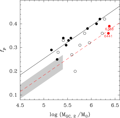
Figure 11.— The fraction of GC mass comprised of pure processed material, $f_{\rm p}$, versus GC mass at an age of 2 Gyr for the Galactic GCs in the sample of Conroy (2012). Filled circles represent GCs with $\mbox{[Fe/H]}>-1.5$, whereas open circles represent more metal-poor GCs. The two most metal-rich GCs in this sample (NGC 6388 and NGC 6441) are shown in red and labeled. The solid line represents a best-fit linear relation for the GCs with $\mbox{[Fe/H]}>-1.5$ except NGC 6388 and NGC 6441. The dashed line is the same as the solid line after shifting it down by 0.07 dex. An estimate of the area expected to be populated by the Magellanic Cloud clusters in our sample is shown in grey. See discussion in § 6.5.

Figure 11 shows $f_{\rm p}$ as a function of ${\cal{M}}_{\rm GC,\,2}$. Different symbols represent GCs with different [Fe/H]. As reported by Conroy (2012) for current GC masses, there is a strong linear correlation between $\log\,({\cal{M}}_{\rm GC,\,2})$ and $f_{\rm p}$, which is generally stronger for the “metal-rich” Galactic GCs (those with [Fe/H] $>-1.5$) than for the metal-poor ones. However, the two most metal-rich Galactic GCs in the compilation of Conroy (2012) (i.e., NGC 6388 ([Fe/H] = $-$0.40) and NGC 6441 ([Fe/H = $-$0.34)) turn out to feature $f_{\rm p}$ values that are systematically below the relation defined by the other “metal-rich” GCs (by $\simeq 0.07\;\mbox{dex}\simeq 5\sigma$). We suggest that this is a manifestation of the metallicity dependence of Oxygen yields in AGB models. The recent models of Ventura et al. (2013) show this quite clearly. In their $Z=0.008$ models, the mean [O/Fe] yield for AGB stars with masses in the range 4 – 8 $M_{\odot}$ is 0.00 $\pm$ 0.02. At metallicities such as those of NGC 6388 and NGC 6441, the full range of [O/Fe] is therefore expected to be near zero, while this range commonly exceeds 1 dex for high-mass low-metallicity GCs (see, e.g., Carretta et al., 2010; Conroy, 2012). Note however that in contrast with [O/Fe], the predicted range of [Na/Fe] in $Z=0.008$ models is similar to that of lower-metallicity models (Ventura et al., 2013). Hence, it seems fair to postulate that the relatively low values of $f_{\rm p}$ for NGC 6388 and NGC 6441 are due to a relative lack of variation in [O/Fe]. Since $Z=0.008$ is also the metallicity of the LMC clusters, one might expect their $f_{\rm p}$ to be similarly low relative to the trend with mass defined by the “metal-rich” Galactic GCs (after removing NGC 6388 and NGC 6441).

The grey area shown in Figure 11 depicts the expected $f_{\rm p}$ values for the clusters in our sample (with $4.5\lesssim\log\,({\cal{M}}_{\rm cl}/M_{\odot})\lesssim 5.4$), under the assumptions mentioned above and allowing for measurement uncertainties similar to those of the Galactic GCs. For a relatively massive cluster in our sample with $5.0\lesssim\log\,({\cal{M}}_{\rm cl}/M_{\odot})\lesssim 5.4$, one would then expect $f_{\rm p}$ to be in the approximate range 0.18 – 0.24 in case star formation occurred in situ in these clusters. (Note that if cluster-GMC merging occurred in the early life of these clusters, the seed clusters would have had a lower mass than in the “in situ” case, so that the expected $f_{\rm p}$ values would be smaller.) The two Galactic GCs in the sample of Conroy (2012) with $f_{\rm p}$ values in this approximate range are NGC 6397 ($f_{\rm p}=0.20$) and NGC 6838 ($f_{\rm p}=0.25$). Defining $\Delta$ [Na/Fe] as the FWHM of a Gaussian fit to the distribution of [Na/Fe] of RGB stars in a given cluster, the data in Table 9 of Carretta et al. (2009) yield $\Delta$ [Na/Fe] = 0.38 dex for both NGC 6397 and NGC 6838. We suggest that this is a suitable estimate for an upper limit of $\Delta$ [Na/Fe] in the clusters in our sample.

The currently available data on $\Delta$ [Na/Fe] for intermediate-age clusters in the Magellanic Clouds consist of elemental abundance measurements of 35 RGB stars in 5 LMC clusters, covering 5 – 11 stars per cluster (Mucciarelli et al., 2008, 2014). Four of their five clusters are members of our sample. We approximate $\Delta$ [Na/Fe] for these clusters by means of the FWHM of Gaussian fits to the distributions of [Na/Fe]. The measurement uncertainty of $\Delta$ [Na/Fe] is approximated by $\sigma_{\rm meas}/\sqrt{(}N_{\ast}-1)$ where $\sigma_{\rm meas}$ is the typical measurement uncertainty of [Na/Fe] of single stars and $N_{\ast}$ is the number of stars measured in a given cluster. Figure 12 shows $\Delta$ [Na/Fe] as a function of the cluster mass. For NGC 1978, we estimate its mass from the compilation of integrated-light 2MASS photometry by Pessev et al. (2006), in conjunction with the age and foreground reddening reported by Mucciarelli et al. (2007) and ${\cal{M}}/L$ data from Bruzual & Charlot (2003) for a Salpeter IMF.

Figure 12 shows that the currently available $\Delta$ [Na/Fe] values of the intermediate-age clusters in the Magellanic Clouds range between about 0.1 and 0.6 dex. While these values do not generally seem inconsistent with the expectation based on the cluster mass dependence of $f_{\rm p}$ among Galactic GCs described above, the situation is not yet clear given the significant scatter of $\Delta$ [Na/Fe] among the clusters and the absence of an obvious dependence on cluster mass. It is not clear to what extent this scatter is caused by the small numbers of stars with spectroscopic abundance measurements in these clusters.

Figure 12.— The variation in [Na/Fe] versus cluster mass for intermediate-age LMC clusters. [Na/Fe] data are from Mucciarelli et al. (2008, 2014). NGC numbers of the clusters are labeled next to their data values. The dashed line illustrates $\Delta$ [Na/Fe] = 0.38, the estimated upper limit of $\Delta$ [Na/Fe] for such clusters. See discussion in § 6.5.

Given the importance of a statistically significant inventory of light-element abundance variations in eMSTO clusters in terms of its relevance in the context of formation scenarios of star clusters, it is important to expand the effort of obtaining high-quality spectroscopic measurements of a statistically adequate number of RGB stars in several eMSTO clusters, with the target stars covering a suitable range of distance from the cluster centers. The latter aspect is important since the age of eMSTO clusters is often similar to their half-mass relaxation time, so that one would expect to see differences in the radial distributions of stars of different age (see Goudfrooij et al., 2011b).

7. Concluding Remarks

In an effort to further our understanding of the nature and demography of the eMSTO phenomenon in intermediate-age star clusters in the Magellanic Clouds, we have obtained new deep two-color imaging for 8 such clusters, using the WFC3 instrument aboard HST. We combined the new data with data already available in the HST archive to establish high-quality photometry with the ePSF fitting technique for a complete sample of 18 Magellanic Cloud star clusters with integrated magnitude $V_{\rm tot}^{0}<12.5$ and integrated-light colors that indicate ages between 1 and 2 Gyr. The star clusters in our sample cover a range in present-day mass from about $3\times 10^{4}$ $M_{\odot}$ to $4\times 10^{5}$ $M_{\odot}$. We used isochrones from the Padova family to determine best-fit population parameters for all clusters in our sample, and we evaluated masses and structural parameters for the clusters using King (1962) model fits to the radial distribution of surface number densities. Using Monte-Carlo simulations, we created artificial CMDs for each cluster, showing its morphology if it were a pure SSP (including unresolved binary stars) for comparison with the observed CMDs. Finally, we evaluated central escape velocities ($v_{\rm esc}$) of the clusters as a function of time using dynamical evolution calculations with and without initial mass segregation. Our main conclusions are the following.

1. All star clusters in our sample with ages in the range 1 – 2 Gyr feature eMSTOs, i.e., MSTO regions that are wider than can be accounted for by a SSP. FWHM widths of pseudo-age distributions derived from the eMSTO morphology are found to be equivalent to age spreads of 200 – 550 Myr. In contrast, similar data of two lower-mass star clusters in the same age range reveals significantly narrower MSTOs whose widths are consistent with those of their respective SSP simulations.
   

2. Star clusters featuring eMSTOs and whose pseudo-age distributions indicate the presence of significant numbers of stars in the age range 1.0 – 1.3 Gyr also feature composite red clumps in their CMDs, even though their formal best-fit age is almost always older than 1.3 Gyr. Conversely, star clusters with eMSTOs but without significant numbers of stars with ages $\leq$ 1.3 Gyr do not show composite red clumps. This constitutes evidence that eMSTOs are caused by a range of ages rather than a range of stellar rotation velocities or the presence of interacting binaries.
   

3. We find that $v_{\rm esc}\gtrsim 15$ km s^-1 out to ages of at least 100 Myr for all clusters that feature eMSTOs, while $v_{\rm esc}\lesssim 15$ km s^-1 at all ages for the two lower-mass clusters that do not show eMSTOs. In the context of the “in situ star formation” scenario, the eMSTO phenomenon would only occur in clusters that feature early $v_{\rm esc}$ values that are higher than the wind velocities of the types of stars that have been proposed to provide the material from which second-generation stars can form. Our result would then suggest that the lower limit to such wind velocities is of order 15 km s^-1. This hypothesis is found to be consistent with observed wind velocities of intermediate-mass AGB stars and massive binary stars in the literature. It is also found to be consistent (albeit possibly only marginally) with the absence of eMSTOs in two young star clusters (with ages $\lesssim 300$ Myr) that was recently reported by Bastian & Silva-Villa (2013).
   

4. We find a significant correlation between the FWHM_MSTO, the width of the pseudo-age distributions of eMSTO clusters, and their central escape velocity at an age of 10 Myr, $v_{\rm esc,\,7}$. This correlation persists when plotting FWHM_MSTO versus current central escape velocity, albeit at lower significance. Similar correlations are found between FWHM_MSTO and cluster mass as well. We find that these correlations cannot be reproduced by the effects of a range of stellar rotation velocities within star clusters according to recent models. In particular, the observed MSTO widths of eMSTO clusters are larger than those predicted by the stellar rotation models, especially for the clusters with the larger values of $v_{\rm esc,\,7}$. Furthermore, it is not clear how to explain the absence of eMSTOs in the two lower-mass clusters in the stellar rotation scenario. We therefore argue that the eMSTO phenomenon among intermediate-age star clusters is mainly caused by extended star formation within the cluster, likely from material shed by first-generation stars featuring slow stellar winds and/or chemically pristine material accreted from the ambient ISM at early times.

The overall general picture on the formation process of intermediate-age star clusters featuring eMSTOs that seems to be most consistent with our results is as follows. The masses and central escape velocities of eMSTO clusters in the first few 10⁸ yr seem to have been high enough to accrete a significant amount of “pristine” gas from the surroundings (by slow accretion and/or by merging with GMCs à la Bekki & Mackey 2009) and/or retain a significant fraction of the gas supplied by slow winds of “polluters” (IM-AGB stars and massive binary stars) of the first generation, and accumulate this material at the bottom of the clusters’ potential wells, making it available for secondary star formation. (This is not the case for clusters whose central escape velocities never exceeded about 12 km s^-1.) During the first few hundreds of Myr, clusters with higher escape velocities generally seem to have been able to extend the star formation process for a longer time than clusters with lower escape velocities, possibly by means of ongoing accretion of pristine gas from the ambient ISM, merging with GMCs, and/or retention of enriched wind material from newly formed polluter stars. The star formation era terminated when at least one of two things occured: (a) the gas swept up and/or accumulated by the cluster is exhausted by star formation, or (b) the collective rate of SN events (i.e., “prompt” SN Ia events by first-generation stars and SN II events by second-generation stars) started to be high enough to sweep out the remaining gas in star clusters.

If eMSTO clusters and ancient Galactic GCs share a formation process that involves star formation over a time span of a few 10⁸ yr, a key prediction would be that eMSTO clusters should show some level of light-element abundance variations in a way similar to the Na-O anti-correlations seen among Galactic GCs. We estimated the expected level of [Na/Fe] variations ($\Delta$ [Na/Fe]) in eMSTO clusters by evaluating the masses of Galactic GCs at an age of 2 Gyr by inversely applying their modeled mass-loss rates during the last $\simeq$ 11 Gyr, followed by an extrapolation of the correlation of the observed extents of the Na-O anti-correlations within the GCs with their masses at an age of 2 Gyr. The estimated levels of $\Delta$ [Na/Fe] in the eMSTO clusters are found to be broadly consistent with the currently available spectroscopic data, although there is a significant scatter of $\Delta$ [Na/Fe] among the clusters. It is not clear to what extent this scatter is caused by the small numbers of stars with abundance measurements in these clusters, and we urge the community to expand the effort of obtaining high-quality spectroscopic measurements of a statistically adequate number of RGB stars in several eMSTO clusters, with the target stars covering a suitable range of distance from the cluster centers, thus making sure that stars of different generations (if present) are sampled adequately. Several teams are presently pursuing such spectroscopic studies, whose results are eagerly awaited.

Table 3Derived dynamical parameters of star clusters in our full sample.

	log (${\cal{M}}_{\rm cl}/M_{\odot}$)			$r_{\rm eff}$							MSTO widths
Cluster	Current	10 Myr	10 Myr, seg.	Current	10 Myr	10 Myr, seg.	$v_{\rm esc}$	$v_{\rm esc,\,7}^{\rm noseg}$	$v_{\rm esc,\,7}^{\rm seg}$	$v_{\rm esc,\,7}^{p}$	FWHM	W20
(1)	(2)	(3)	(4)	(5)	(6)	(7)	(8)	(9)	(10)	(11)	(12)	(13)
NGC 411	4.67 $\pm$ 0.03	4.82 $\pm$ 0.03	5.24 $\pm$ 0.03	6.1 $\pm$ 0.8	4.8 $\pm$ 0.6	3.3 $\pm$ 0.4	10.0 $\pm$ 0.8	13.6 $\pm$ 1.0	26.7 $\pm$ string2.1	22.5 $\pm$ string1.6	516	704
NGC 419	5.38 $\pm$ 0.08	5.51 $\pm$ 0.08	5.94 $\pm$ 0.08	7.7 $\pm$ 2.9	6.0 $\pm$ 2.2	4.1 $\pm$ 1.5	20.6 $\pm$ 4.2	26.8 $\pm$ 5.5	53.4 $\pm$ 11.0	53.3 $\pm$ 11.0	560	799
NGC 1651	4.91 $\pm$ 0.06	5.04 $\pm$ 0.06	5.48 $\pm$ 0.06	12.8 $\pm$ 1.0	9.9 $\pm$ 0.8	6.8 $\pm$ 0.5	10.2 $\pm$ 0.7	13.6 $\pm$ 1.3	27.3 $\pm$ string2.7	20.4 $\pm$ string2.5	315	584
NGC 1718	4.83 $\pm$ 0.07	5.01 $\pm$ 0.07	5.43 $\pm$ 0.07	5.4 $\pm$ 0.6	4.2 $\pm$ 0.4	2.9 $\pm$ 0.3	13.0 $\pm$ 1.3	18.1 $\pm$ 1.8	35.5 $\pm$ string3.5	27.8 $\pm$ string2.7	406	650
NGC 1751	4.81 $\pm$ 0.06	4.95 $\pm$ 0.06	5.38 $\pm$ 0.06	7.1 $\pm$ 0.9	5.6 $\pm$ 0.7	3.8 $\pm$ 0.5	10.9 $\pm$ 1.0	14.6 $\pm$ 1.4	29.0 $\pm$ string2.7	25.4 $\pm$ string2.4	353	509
NGC 1783	5.42 $\pm$ 0.11	5.54 $\pm$ 0.11	5.98 $\pm$ 0.01	11.4 $\pm$ 2.2	8.9 $\pm$ 1.7	6.1 $\pm$ 1.2	17.6 $\pm$ 1.8	23.0 $\pm$ 2.4	46.0 $\pm$ string4.8	39.9 $\pm$ string4.2	403	584
NGC 1806	5.10 $\pm$ 0.06	5.23 $\pm$ 0.06	5.66 $\pm$ 0.06	9.0 $\pm$ 1.2	7.0 $\pm$ 1.0	4.8 $\pm$ 0.7	13.7 $\pm$ 1.0	18.0 $\pm$ 1.4	35.9 $\pm$ string2.7	31.4 $\pm$ string2.4	370	613
NGC 1846	5.24 $\pm$ 0.09	5.37 $\pm$ 0.09	5.80 $\pm$ 0.09	8.8 $\pm$ 0.7	6.8 $\pm$ 0.5	4.7 $\pm$ 0.4	16.3 $\pm$ 1.9	21.5 $\pm$ 2.6	42.9 $\pm$ string5.1	35.8 $\pm$ string4.6	567	757
NGC 1852	4.66 $\pm$ 0.07	4.81 $\pm$ 0.07	5.24 $\pm$ 0.07	7.0 $\pm$ 0.8	5.5 $\pm$ 0.7	3.7 $\pm$ 0.4	9.4 $\pm$ 0.9	12.6 $\pm$ 1.2	24.9 $\pm$ string2.4	23.7 $\pm$ string2.2	312	432
NGC 1987	4.74 $\pm$ 0.04	4.85 $\pm$ 0.04	5.26 $\pm$ 0.04	12.8 $\pm$ 3.0	10.1 $\pm$ 2.4	6.9 $\pm$ 1.6	8.7 $\pm$ 1.2	11.1 $\pm$ 1.8	21.7 $\pm$ string3.6	20.4 $\pm$ string3.4	234	424
NGC 2108	4.71 $\pm$ 0.07	4.84 $\pm$ 0.07	5.24 $\pm$ 0.07	7.2 $\pm$ 0.8	5.7 $\pm$ 0.6	3.9 $\pm$ 0.4	9.8 $\pm$ 0.9	12.7 $\pm$ 1.2	24.5 $\pm$ string2.3	21.3 $\pm$ string2.0	230	359
NGC 2154	4.61 $\pm$ 0.06	4.80 $\pm$ 0.06	5.21 $\pm$ 0.06	5.7 $\pm$ 0.5	4.4 $\pm$ 0.4	3.0 $\pm$ 0.3	9.9 $\pm$ 0.8	13.7 $\pm$ 1.1	26.9 $\pm$ string2.1	23.6 $\pm$ string1.9	431	625
NGC 2173	4.67 $\pm$ 0.07	4.83 $\pm$ 0.07	5.26 $\pm$ 0.07	6.3 $\pm$ 1.1	4.9 $\pm$ 0.9	3.4 $\pm$ 0.6	11.4 $\pm$ 1.3	13.8 $\pm$ 1.7	27.2 $\pm$ string3.3	22.7 $\pm$ string3.5	431	589
NGC 2203	4.95 $\pm$ 0.07	5.08 $\pm$ 0.07	5.51 $\pm$ 0.07	9.5 $\pm$ 1.6	7.4 $\pm$ 1.2	5.1 $\pm$ 0.8	11.2 $\pm$ 1.3	14.8 $\pm$ 1.7	29.4 $\pm$ string3.4	25.5 $\pm$ string2.9	475	652
NGC 2213	4.46 $\pm$ 0.05	4.74 $\pm$ 0.05	5.13 $\pm$ 0.05	3.6 $\pm$ 0.3	2.8 $\pm$ 0.2	1.9 $\pm$ 0.2	10.4 $\pm$ 0.6	16.4 $\pm$ 1.0	30.8 $\pm$ string1.9	20.2 $\pm$ string1.2	329	502
LW 431	4.56 $\pm$ 0.07	4.68 $\pm$ 0.07	5.11 $\pm$ 0.07	9.1 $\pm$ 3.2	7.1 $\pm$ 2.5	4.9 $\pm$ 1.7	7.8 $\pm$ 1.5	10.0 $\pm$ 2.2	19.9 $\pm$ string4.3	17.2 $\pm$ string3.7	277	462
Hodge 2	4.70 $\pm$ 0.07	4.83 $\pm$ 0.07	5.25 $\pm$ 0.07	9.1 $\pm$ 2.3	7.2 $\pm$ 1.8	4.9 $\pm$ 1.3	10.2 $\pm$ 1.5	13.3 $\pm$ 2.4	26.1 $\pm$ string4.7	19.3 $\pm$ string3.5	363	520
Hodge 6	4.74 $\pm$ 0.07	4.94 $\pm$ 0.07	5.37 $\pm$ 0.07	5.5 $\pm$ 0.9	4.3 $\pm$ 0.7	2.9 $\pm$ 0.5	11.6 $\pm$ 1.3	16.6 $\pm$ 1.8	32.8 $\pm$ string3.6	21.0 $\pm$ string3.0	$<$238	$<$435

Note. — Column (1): name of star cluster. Column (2): integrated $V$-band magnitude. Column (3): radius of aperture used for integrated-light photometry in arcsec. Column (4): reference of integrated-light photometry (1 = Goudfrooij et al. 2006; 2 = Bica et al. 1996). Column (5): core radius in pc. Column (6): effective radius in pc. Column (7): (mean) age in Gyr. Column (8): metallicity in dex. Column (9): $V$-band foreground extinction. Column (10): distance modulus. Column (11): reference of data in columns 5 – 10 (1 = this paper; 2 = Goudfrooij et al. 2011a).

Note. — Column (1): Name of star cluster. (2): Date of HST/WFC3 observations. (3) Total exposure time in F475W filter in seconds. (4): total exposure time in F814W filter.

Note. — Column (1): relation being tested. Column (2): probability of an absence of a correlation according to the Cox Proportional Hazard Model test. Column (3): value of generalized Kendall’s correlation coefficient. Column (4): $Z$-value of generalized Kendall’s correlation test. Column (5): probability of an absence of a correlation according to the generalized Kendall’s correlation test. See discussion in § 5.5.

Note. — Columns: (1): GC ID; (2): [Fe/H] in dex; (3): Number of stars used in the abundance analysis (see Conroy 2012); (4): Log of current GC mass in $M_{\odot}$. (5): mass fraction of processed material ; (6): Effective radius from Harris (1996) in pc; (7): log of GC mass at age of 2 Gyr in $M_{\odot}$.

Note. — Column (1): Name of star cluster. (2): Logarithm of adopted current cluster mass (in solar masses). (3): Logarithm of adopted cluster mass at an age of 10 Myr (no initial mass segregation case). (4): same as (3), but for max. initial mass segregation case. (5) Current cluster half-mass radius in pc. (6): Adopted cluster half-mass radius at an age of 10 Myr (no initial mass segregation case). (7): same as (6), but for max. initial mass segregation case. (8): Current central cluster escape velocity in km s^-1. (9): Central cluster escape velocity at an age of 10 Myr (no initial mass segregation case). (10): same as (8), but for max. initial mass segregation case. (11): same as (9), but for “plausible” level of initial mass segregation (see § 5.5). (12): Value of FWHM_MSTO in Myr. (13): Value of W20_MSTO in Myr.

References

- Anderson et al. (2008) Anderson, J., Sarajedini, A., Bedin, L. R., et al. 2008, AJ, 135, 2055
- Bastian et al. (2013b) Bastian, N., Cabrera-Ziri, I., Davies, B., & Larsen, S. S. 2013b, MNRAS, 436, 2852
- Bastian & de Mink (2009) Bastian, N., & de Mink, S. E. 2009, MNRAS, 398, L11
- Bastian et al. (2013a) Bastian, N., Lamers, H. J. G. L. M., de Mink, S. E., et al. 2013a, MNRAS, 436, 2398