Relational Linear Programs

Abstract

We propose relational linear programming, a simple framework for combing linear programs (LPs) and logic programs. A relational linear program (RLP) is a declarative LP template defining the objective and the constraints through the logical concepts of objects, relations, and quantified variables. This allows one to express the LP objective and constraints relationally for a varying number of individuals and relations among them without enumerating them. Together with a logical knowledge base, effectively a logical program consisting of logical facts and rules, it induces a ground LP. This ground LP is solved using lifted linear programming. That is, symmetries within the ground LP are employed to reduce its dimensionality, if possible, and the reduced program is solved using any off-the-shelf LP solver. In contrast to mainstream LP template languages like AMPL, which features a mixture of declarative and imperative programming styles, RLP’s relational nature allows a more intuitive representation of optimization problems over relational domains. We illustrate this empirically by experiments on approximate inference in Markov logic networks using LP relaxations, on solving Markov decision processes, and on collective inference using LP support vector machines.

1 Introduction

Modern social and technological trends result in an enormous increase in the amount of accessible data, with a significant portion of the resources being interrelated in a complex way and having inherent uncertainty. Such data, to which we may refer to as relational data, arise for instance in social network and media mining, natural language processing, open information extraction, the web, bioinformatics, and robotics, among others, and typically features substantial social and/or business value if become amenable to computing machinery. Therefore it is not surprising that probabilistic logical languages, see e.g. [GT07, De 08, DFKM08, RK10] and references in there for overviews, are currently provoking a lot of new AI research with tremendous theoretical and practical implications. By combining aspects of logic and probabilities — a dream of AI dating back to at least the late 1980s when Nils Nilsson introduced the term probabilistic logics [Nil86] — they help to effectively manage both complex interactions and uncertainty in the data. Moreover, since performing inference using traditional approaches within these languages is in principle rather costly, as tractability of traditional inference approaches comes at the price of either coarse approximations (often without any guarantees) or restrictions in the language, they have motivated novel forms of inference. In essence, probabilistic logical models can be viewed as collections of building blocks respectively templates such as weighted clauses that are instantiated several times to construct a ground probabilistic model. If few templates are instantiated often, the resulting ground model is likely to exhibit symmetries. In his seminal paper [Poo03], David Poole suggested to exploited these symmetries to speed up inference within probabilistic logic models. This has motivated an active field of research known as lifted probabilistic inference, see e.g. [Ker12] and references in there.

However, instead of looking at AI through the glasses of probabilities over possible worlds, we may also approach it using optimization. That is, we have a preference relation over possible worlds, and we want a best possible world according to the preference. The preference is often to minimize some objective function. Consider for example a typical machine learning user in action solving a problem for some data. She selects a model for the underlying phenomenon to be learned (choosing a learning bias), formats the raw data according to the chosen model, and then tunes the model parameters by minimizing some objective function induced by the data and the model assumptions. In the process of model selection and validation, the core optimization problem in the last step may be solved many times. Ideally, the optimization problem solved in the last step falls within a class of mathematical programs for which efficient and robust solvers are available. For example, linear, semidefinite and quadratic programs, found at the heart of many popular AI and learning algorithms, can be solved efficiently by commercial-grade software packages.

This is an instance of the declarative “$\text{Model}+\text{Solver}$” paradigm currently observed a lot in AI [Gef14], machine learning and also data mining [GND11]: instead of outlining how a solution should be computed, we specify what the problem is using some high-level modeling language and solve it using general solvers.

Unfortunately, however, today’s solvers for mathematical programs typically require that the mathematical program is presented in some canonical algebraic form or offer only some very restricted modeling environment. For example, a solver may require that a set of linear constraints be presented as a system of linear inequalities $\mathbf{A}\mathbf{x}\leq\mathbf{b}$ or that a semidefinite constraint be expressed as $\sum_{i}\mathbf{y}_{i}\mathbf{A}_{i}\succeq\mathbf{C}$. This may create severe difficulties for the user:

1. Practical optimization involves more than just the optimization of an objective function subject to constraints. Before optimization takes place, effort must be expended to formulate the model. This process of turning the intuition that defines the model “on paper” into a canonical form could be quite cumbersome. Consider the following example from graph isomorphism, see e.g. [AM13]. Given two graphs $G$ and $H$, the LP formulation introduces a variable for every possible partial function mapping $k$ vertices of $G$ to $k$ vertices in $H$. In this case, it is not a trivial task to even come up with a convenient linear indexing of the variables, let alone expressing the resulting equations as $\mathbf{A}\mathbf{x}\leq\mathbf{b}$. Such conversions require the user to produce and maintain complicated matrix generation code, which can be tedious and error-prone. Moreover, the reusability of such code is limited, as relatively minor modification of the equations could require large modifications of the code (for example, the user decides to switch from having variables over sets of vertices to variables over tuples of vertices). Ideally, one would like to separate the problem specification from the problem instance itself

2. Canonical forms are inherently propositional. By design they cannot model domains with a variable number of individuals and relations among them without enumerating all of them. As already mentioned, however, many AI tasks and domains are best modeled in terms of individuals and relations. Agents must deal with heterogenous information of all types. Even more important, they must often build models before they know what individuals are in the domain and, therefore, before they know what variables exist. Hence modeling should facilitate the formulation of abstract, general knowledge.

To overcome these downsides and triggered by the success of probabilistic logical languages, we show that optimization is liftable to the relational level, too. Specifically, we focus on linear programs which are the most tractable, best understood, and widely used in practice subset of mathematical programs. Here, the objective is linear and the constraints involve linear (in)equalities only. Indeed, at the inference level within propositional models considerable attention has been already paid to the link between probabilistic models and linear programs. This relation is natural since the MAP inference problem can be relaxed into linear programs. At the relational and lifted level, however, the link has not been established nor explored yet.

Our main contribution is to establish this link, both at the language and at the inference level. We introduce relational linear programming best summarized as

$$\big{(}(\text{LP}+\text{Logic})-\text{Symmetry}\big{)}+\text{Solver}.$$

The user describes a relational problem in a high level, relational LP modeling language and — given a logical knowledge base (LogKB) encoding some individuals or rather data — the system automatically induces a symmetry-reduced LP that in turn can be solved using any off-the-shelf LP solver. Its main building block are relational linear programs (RLPs). They are declarative LP templates defined through the logical concepts of individuals, relations, and quantified variables and allow the user to express the LP objective and constraints about a varying number of individuals without enumerating them. Together with a the LogKB referring to the individuals and relations, effectively a logical program consisting of logical facts and rules, it induces a ground LP. This ground LP can be solved using any LP solver. Our illustrations of relational linear programming on several AI problems will showcase that relational programming can considerably ease the process of turning the “modeller’s form” — the form in which the modeler understands a problem or actually a class of problems — into a machine readable form since we can now deal with a varying number of individuals and relational among them in a declarative way. We will show this for computing optimal value function of Markov decision processes [LDP95], for approximate inference within Markov logic networks [RD06] using LP relaxations as well as for collective classification [SNB⁺08a].

In particular, as another contribution, we will showcase a novel approach to collective classification by relational linear programming. Say we want to classify people as having or not having cancer. In addition to the usual “flat” data about attributes of people like age, education and smoking habits, we have access to the social network among the people, cf. Fig. 1. This allows us to model influence among smoking habits among friend. Now imagine that we want to do the classification using support vector machines (SVMs) [Vap98] which boils down to a quadratic optimization problem. Zhou et. al. [ZZJ02] have shown that the same problem can be modeled as an LP with only a small loss in generalization performance. Existing LP template language, however, would require feature engineering to capture smoking habits among friend. In contrast, in an RLP one simply adds rules such as

$$\mathtt{attribute(X,passive)\ \operatorname{:-}\ friends(X,Y),attribute(Y,smokes)}$$

saying that if two persons $\mathtt{X}$ and $\mathtt{Y}$ are friends and $\mathtt{Y}$ smokes, then $\mathtt{X}$ also smokes, at least passively. Moreover, as we will do in our experiments, we can formulate relational LP constraints to encode that objects that link to each other tend to be in the same class.

(a)

name	age	education	smokes
anna	27	uni	+
bob	22	college	-
edward	25	college	-
frank	30	uni	-
gary	45	college	+
helen	35	school	+
iris	50	school	-

(b)

Figure 1: Example for collective inference. There are $7$ people in a social network. Each person is described in terms of three attributes. The class label “cancer” is not shown.

However, the benefits of relational linear programming go beyond modeling. Since RLPs consist of templates that are instantiated several times to construct a ground linear model, they are also likely to induce ground models that exhibit symmetries, and we will demonstrate how to detect and exploit them. Specifically, we will introduce lifted linear programming (LLP). It detects and eliminates symmetries in a linear program in quasilinear time. Unlike lifted probabilistic inference methods such as lifted belief propagation [SD08, KAN09, AKMN13], which works only with belief propagation approximations for probabilistic inference, LLP does not depend on any specific LP solver — it can be seen as simply reparametrizing the linear program. As our experimental results on several AI tasks will show this can result in significant efficiency gains.

We proceed as follows. After touching upon related work, we start off by reviewing linear programming and existing LP template languages in Section 3. Then, in Section 4, we introduce relational linear programming, both the syntax and the semantics. Afterwards, Section 5 shows how to detect and exploit symmetries in linear programs. Before touching upon directions for future work and concluding, we illustrate relational linear programming on several examples from machine learning and AI.

2 Related Work on Relational and Lifted Linear Programming

The present paper is a significant extension of the AISTATS 2012 conference paper [MAK12]. It provides a much more concise development of lifted linear programming compared to [MAK12] and the first coherent view on relational linear programming as a novel and promising way for scaling AI. To do so, it develops the first relational modeling language for LPs and illustrates it empirically. One of the advantages of the language is the closeness of its syntax to the mathematical notation of LP problems. This allows for a very concise and readable relational definition of linear optimization problems, which is supported by certain language elements from logic such as individuals, relations, and quantified variables. The (relational) algebraic formulation of a model does not contain any hints how to process it. Indeed, several modeling language for mathematical programming have been proposed. Examples of popular modeling languages are AMPL [FGK93], GAMS [BKM92], AIMMS [BL93], and Xpress-Mosel [CCH03], but also see [Kui93, FG02, WZ05] for surveys. Although they are declarative, they focus on imperative programming styles to define the index sets and data tables typically used to construct LP model. They do not employ logical concepts such as clauses and unification. Moreover, since index sets and data tables are closely related to the attributes and relations of relational database systems, there have been also proposals for “feeding” linear program directly from relational database systems, see e.g. [MdSMK95, AJLS00, FM05]. However, logic programming — which allows to use e.g. compound terms — was not considered and the resulting approaches do not provide a syntax close to the mathematical notation of linear programs. Recently, Mattingley and Boyd [MB12] have introduced CVXGEN, a software tool that takes a high level description of a convex optimization problem family, and automatically generates custom C code that compiles into a reliable, high speed solver for the problem family. Again concepts from logic programing were not used. Indeed, Gordon et al. [GHD09, ZGP11] developed first-order programming (FOP) that combines the strength of mixed-integer linear programming and first-order logic. In contrast to the present paper, however, they focused on first-order logical reasoning and not on specifying relationally and solving efficiently arbitrary linear programs. And non of these approaches as considered symmetries in LPs and how to detect and to exploit them.

Indeed, detection and exploiting symmetries within LPs is related to symmetry-aware approaches in (mixed–)integer programming [Mar10]. Howerver, they are vastly different to LPs in nature. Symmetries in ILP are used for pruning the symmetric branches of search trees, thus the dominant paradigm is to add symmetry breaking inequalities, similarly to what has been done for SAT and CSP [SV05]. In contrast, lifted linear programming achieves speed-up by reducing the problem size. For ILPs, symmetry-aware methods typically focus on pruning the search space to eliminate symmetric solutions, see e.g. [Mar10] for a survey). In linear programming, however, one takes advantage of convexity and projects the LP into the fixed space of its symmetry group [BHJ13]. The projections we investigate in the present paper are similar in spirit. Until recently, discussions were mostly concentrated on the case where the symmetry group of the ILP/LP consists of permutations, e.g. [BGH10]. In such cases the problem of computing the symmetry group of the LP can be reduced to computing the coloured automorphisms of a “coefficient” graph connected with the linear program, see e.g. [BP09, Mar10]. Moreover, the reduction of the LP in this case essentially consists of mapping variables to their orbits. Our approach subsumes this method, as we replace the orbits with a coarser equivalence relation which, in contrast to the orbits, is computable in quasilinear time. Going beyond permutations, Bödi and Herr [BHJ13] extend the scope of symmetry, showing that any invertible linear map, which preserves the feasible region and objective of the LP, may be used to speed-up solving. While this setting offers more compression, the symmetry detection problem becomes even more difficult.

After the AISTATS conference paper [MAK12], lifted (I)LP-MAP inference approaches for (relational) graphical models based on graph automorphisms and variants have been explored in several ways, which go beyond the scope of the present paper. We refer to [BHR13, NNS13, MGK14, AKM14].

3 Linear Programming

Linear programs, see e.g. [DT03], have found a wide application in the fields of operations research, where they are applied to problems like multicommodity flow and optimal resource allocation, and combinatorial optimization, where they provide the basis for many approximation algorithms for hard problems such as TSP. They have also found their way to machine learning and AI. Consider e.g. support vector machine (SVMs), which are among the most popular models for classification. Although they are traditionally formulated as quadratic optimization problems, there are also linear program (LP) formulations of SVMs such as Zhou et al.’s LP-SVMs [ZZJ02]. Many other max-margin approaches use LPs for inference as well such as LP boosting [DBST02] or LP-based large margin structure prediction [WS09]. They have also been used for the decoding step within column generation approaches to solving quadratic problem formulations of the collective classification task, see e.g. [KBS08, TL13] and reference in there. However, they are not based on LP-SVMs and on relational programming. In probabilistic graphical models LP relaxations are used for efficient approximate MAP inference, see e.g. [WJ08]. Finding the optimal policy for a Markov decision problem can be formulated and solved with LPs [SBS08]. Likewise, they have been used for inverse reinforcement learning [NR⁺00] where the goal is to estimate a reward function from observed behaviour. In addition, recent work use approximate LPs for relational MDPs [SB09], which scale to problems of previously prohibitive size by avoiding grounding. However, they were not using relational LPs. Clustering can also be formulated via LPs, see e.g. [KPT08]. Ataman applied LPs to learning optimal rankings for binary classification problems [ASZ06]. In many cases, even if a learning problem itself is not posed as an LP, linear programming is used to solve some intermediate steps. For instance Sandler et al. [San05] phrases computing the pseudoinverse of a matrix and greedy column selection from this pseudoinverse as LPs. The resulting matrix is then used for dimensionality reduction and unsupervised text classification. So what are linear programs?

3.1 Linear Programs

A linear program (LP) is an optimization problem that can be expressed in the following general form:

$$\operatorname*{minimize}\nolimits_{\mathbf{x}\in\mathbb{R}^{n}} \left<\mathbf{c},\mathbf{x}\right>$$

subject to $$\mathbf{A}\mathbf{x}\leq\mathbf{b}$$

$$\mathbf{G}\mathbf{x}=\mathbf{h}\;,$$

where $\mathbf{A}\in\mathbb{R}^{m\times n}$ and $\mathbf{G}\in\mathbb{R}^{p\times n}$ are matrices, $\mathbf{b},\ \mathbf{c}$ and $\mathbf{h}$ are real vectors of dimension $m,n,$ and $p$ respectively, and $\left<\cdot,\cdot\right>$ denotes the inner product of two vectors. Note that the equality constraints can be reformulated as inequality constraints to yield an LP in the so-called dual form,

$$\operatorname*{minimize}\nolimits_{\mathbf{x}\in{\mathbb{R}}^{n}} \left<\mathbf{c},\mathbf{x}\right>$$ (1)

subject to $$\mathbf{A}\mathbf{x}\leq\mathbf{b}\;,$$

which we represent by the triplet $L=(\mathbf{A},\mathbf{b},\mathbf{c})$.

While LP models often look intuitive on paper, applying these models in practice presents a challenge. The main issue is that the form of a problem representation that is natural for most solvers (i.e. the L triplet representation) is not the form that is natural for domain experts. Furthermore, the matrix $\mathbf{A}$ is typically sparse, i.e., having mostly $0$-entries. Modeling any real world problem in this form can be quite error prone and time consuming. In addition, it is often necessary to separate the general structure of a problem from the definition of a particular instance. For example, a flow problem formulated as an LP consists of a set of constraint for each edge in a graph, which do not depend on a particular graph. Hence, the definition of the flow LP can be separated from the specification of the graph at hand and, in turn, be applied to different graphs.

3.2 Declarative Modelling Languages for Linear Programs

The problems above are traditionally solved by modelling languages. They simplify LP definition by allowing to use algebraic notation instead of matrices and define an objective and constraints through parameters whose domains are defined in a separate file, thus enabling model/instance separation. Starting from Eq. 1, they typically make the involved arithmetic expressions explicit:

$$\operatorname*{minimize}\nolimits_{\mathbf{x}\in\mathbb{R}^{n}} \sum\nolimits_{j\in P}c_{j}x_{j}$$ (2)

subject to $$\sum\nolimits_{j\in P}a_{ij}x_{j}\leq b_{i}\text{ for each }i\in K\;,$$

where the sets ${P}$ and ${K}$ as well as the corresponding non-zero entries of vectors ${\mathbf{c}}$, ${\mathbf{b}}$ and matrix ${\mathbf{A}}$ are defined in a separate file. This simplified representation is then automatically translated to the matrix format and fed to a solver that the user prefers.

To code the LP in this “set form”, several mathematical programming modelling languages have been proposed to implement this general idea. According to NEOS solver statistics, AMPL is the most popular one. We only briefly review the basic AMPL concepts. For more details, we refer to  [FGK93].

Based on the “set form”, an LP can be written in AMPL as shown in Fig. 2.

⬇

1set P; #column dimension of A

2set K; #row dimension of A

3param a {j in P, i in K}; #provided as input

4param c {j in P}; #provided as input

5param b {i in K}; #provided as input

6var x {j in P}; #determined by the solver

7

8#the objective

9minimize: sum {j in P} c[j] * x[j];

10#the constraints

11subject to sum {j in P} a[i, j]*x[j] <= b[i];

Figure 2: AMPL declaration scheme for a linear program in “set form” as shown in Eq. 2.

In principle an AMPL program consists of one objective and a number of ground or indexed constraints. If a constrain is indexed, (i.e. the constraint in the example above is indexed by the set K) a ground constraint is generated for every combination of values of index variables (in the example above there is just one index variable in the constrain, hence a ground constraint is generated for every value in K). The keyword set declares a set name, whose members are provided in a separate file. The keyword param declares a parameter, which may be a single scalar value or a collection of values indexed by a set. Subscripts in algebraic notation are written in square brackets as in b[i] instead of ${b_{i}}$. The values to be determined by the solver are defined by the var keyword. The typical ${\sum}$ symbol is replaced by the sum keyword. The key element of the AMPL system is the so called indexing expression

$$\mathtt{\{j\ in\ P\}}\;.$$

In addition to being a part of variable/parameter declaration, they serve both as limits for sums and as indices for constraints. Finally, comments in AMPL start with the symbol #.

In relational linear programs, which we will introduce next, we are effectively mixing first order logic into AMPL. This allows us to keep AMPL’s benefits that make it the number one choice for optimization experts and at the same time enable the representation of relational problems.

4 Relational Linear Programming

The main idea of relational linear programming is to parameterize AMPL’s arithmetic expressions by logical variables and to replace AMPL’s indexing expression by queries to a logical knowledge base. Before showing how to do this, let us briefly review logic programming. For more details we refer to [Llo87, Fla94, De 08].

4.1 Logic Programming

A logic program is a set of clauses constructed using four types of symbols: constants, variables, functors, and predicates. Reconsider the collective classification example from the introduction, also see in Fig. 1, and in particular the “passive smoking” rule. Formally speaking, we have that $\mathtt{attribute/2}$ $\mathtt{friends/2}$ are predicates (with their arity, i.e., number of arguments listed explicitly). The symbols anna, bob, edward, frank, gary, helen, iris are constants and $\mathtt{X}$, and $\mathtt{Y}$ are variables. All constants and variables are also terms In addition, one can also have structured terms such as $\mathtt{s(X)}$, which contains the functor $\mathtt{s/1}$ of arity $1$ and the term $\mathtt{X}$. Atoms are predicate symbols followed by the necessary number of terms, e.g., $\mathtt{friends(bob,anna)}$, $\mathtt{nat(s(X))}$, $\mathtt{attribute(X,passive)}$, etc. Literals are atoms $\mathtt{nat(s(X))}$ (positive literal) and their negations $\mathtt{not\ nat(s(X))}$ (negative literals). We are now able to define the key concept of a clause. They are formulas of the form

$$\mathtt{A\operatorname{:-}B_{1},\ldots,B_{m}}$$

where $\mathtt{A}$ – the head – and the $\mathtt{B_{j}}$ — the body — are logical atoms and all variables are understood to be universally quantified. For instance, the clause

$$c\equiv{\mathtt{attribute(X,passive)\operatorname{:-}friends(X,Y),attribute(Y,smokes)}}$$

can be read as $\mathtt{X}$ has $\mathtt{attribute}$ $\mathtt{passive}$ if $\mathtt{X}$ and $\mathtt{Y}$ are $\mathtt{friends}$ and $\mathtt{Y}$ has the $\mathtt{attribute}$ $\mathtt{smokes}$. Clauses with an empty body are facts. A logic program consists of a finite set of clauses. The set of variables in a term, atom, conjunction or clause $E$, is denoted as $\operatorname{Var}(E)$, e.g., $\operatorname{Var}(c)=\{\mathtt{X},\mathtt{Y}\}$. A term, atom or clause $E$ is ground when there is no variable occurring in $E$, i.e. $\operatorname{Var}(E)=\emptyset$. A clause $c$ is range-restricted when all variables in the left-hand side of $\operatorname{:-}$ also appear in the right-hand side.

A substitution ${\theta=\{V_{1}/t_{1},\ldots,V_{n}/t_{n}\}}$, e.g. $\{\mathtt{Y}/\mathtt{anna}\}$, is an assignment of terms $t_{i}$ to variables $V_{i}$. Applying a substitution $\theta$ to a term, atom or clause $e$ yields the instantiated term, atom, or clause $e\theta$ where all occurrences of the variables $V_{i}$ are simultaneously replaced by $t_{i}$, e.g. $c\{\mathtt{Y}/\mathtt{anna}\}$ is

$${\mathtt{attribute(X,passive)\operatorname{:-}friends(X,anna),attribute(anna,smokes)}}\;.$$

The Herbrand base of a logic program $P$, denoted as $\operatorname{hb}(P)$, is the set of all ground atoms constructed with the predicate, constant and function symbols in the alphabet of $P$. A Herbrand interpretation for a logic program $P$ is a subset of $\operatorname{hb}(P)$. A Herbrand interpretation $I$ is a model of a clause $c$ if and only if for all substitutions $\theta$ such that $\operatorname{body}(c)\theta\subseteq I$ holds, it also holds that $\operatorname{head}(c)\theta\in I$. A clause $c$ (logic program $P$) entails another clause $c^{\prime}$ (logic program $P^{\prime}$), denoted as $c\models c^{\prime}$ ($P\models P^{\prime}$), if and only if, each model of $c$ ($P$) is also a model of $c^{\prime}$ ($P^{\prime}$).

The least Herbrand model $\operatorname{LH}(P)$, which constitutes the semantics of the logic program $P$, consists of all facts $f\in\operatorname{hb}(P)$ such that $P$ logically entails $f$, i.e. $P\models f$. Answering a query $q\equiv\mathtt{\operatorname{:-}G_{1},G_{2}\ldots,G_{n}}$ with respect to a logic program is to determine whether the query is entailed by the program or not. That is, $q$ is true in all worlds where $P$ is true. This is often done by refutation: $P$ entails $q$ iff ${P\cup\lnot q}$ is unsatisfiable.

Logic programming is especially convenient for representing relational data like the social graph in Fig. 1. All one needs is the binary predicate friend/2 to encode the edges in the social graph as well as the predicate ${\tt attribute(X,Attr)}$ to code the attributes of the people in the social network.

4.2 Relational Linear Programs

Since our language can be seen as a logic programming variant of AMPL, we introduce its syntax in a contrast to the AMPL syntax. To do so, let us consider a well known network flow problem [AMO93]. The problem is to, given a finite directed graph ${G(V,E)}$ in which every edge ${(u,v)\in E}$ has a non-negative capacity ${c(u,v)}$, and two vertices ${s}$ and ${t}$ called source and sink, maximize a function $f:V\times V\rightarrow\mathbb{R}$ called flow with the first parameter fixed to ${s}$ (outgoing flow from the source node), subject to the following constraints: $f(u,v)\leq c(u,v),\ f(u,v)\geq 0,$ and

$$\sum\nolimits_{w\in V/\{s,t\}}f(u,w)=\sum\nolimits_{w\in V/\{s,t\}}f(w,u)\;,$$

where the third constraint means that incoming flow equals to outgoing flow for internal vertices. Such flow problems can naturally be formulated as an LP specified in AMPL as shown in Fig. 3.

⬇

1set VERTEX; #vertices

2set EDGES within (VERTEX diff {sink}) cross (VERTEX diff {source}); #edges

3

4param source symbolic in VERTEX; #entrance to the graph

5param sink symbolic in VERTEX, <> source; #exit from the graph

6param cap {EDGES} >= 0; #flow capacities

7

8var Flow {(i,j) in EDGES} >= 0, <= cap[i,j]; #flows

9

10maximize: sum {(source,j) in EDGES} Flow[source,j]; #objective

11

12subject to {k in VERTEX diff {source,sink}}: #conservation of flow

13 sum {(i,k) in EDGES} Flow[i,k] = sum {(k,j) in EDGES} Flow[k,j];

Figure 3: AMPL specification for a general flow linear program. The vertices and edges as well as the corresponding flow capacities are provided in separate files. The flows of the edges are declared to be determined by the LP solver.

The program starts with a definition of all sets, parameters and variables that appear in it. They are then used to define the objective and the constraints from the network flow problem, in particular the third one. The first two constraints are incorporated into the variable definition. As one can see, AMPL allows one to write down the problem description in a declarative way. It frees the user from engineering instance specific LPs while capturing the general properties of the problem class at hand. However, AMPL does not provide logically parameterized definitions for the arithmetic expressions and for the index sets. RLPs, which we will introduce now, feature exactly this.

A first important thing to notice is that AMPL mimics arithmetic notation in its syntax as much as possible. It operates on sets, intersections of sets and arithmetic expressions indexed with these sets. Our language for relational linear programming effectively replaces these constructs with logical predicates, clauses, and queries to define the three main parts of an RLP: the objective template, the constraints template, and a logical knowledge base. An RLP for the flow example is shown in Fig. 4. It directly codes the flow constraints, concisely captures the essence of flow problems, and illustrates nicely that linear programming in general can be viewed as being highly relational in nature. Let’s now discuss this program line by line.

⬇

1var flow/2; #the flow along edges is determined by the solver

2

3outflow(X) = sum {edge(X, Y)} flow(X, Y); #outflow of nodes

4inflow(Y) = sum {edge(X, Y)} flow(X, Y); #outflow of nodes

5

6maximise: sum {source(X)} outflow(X); #objective

7

8subject to {vertex(X), not source(X), not sink(X)}: #conservation of flow

9 outflow(X) - inflow(X) = 0;

10subject to {edge(X, Y)}: cap(X, Y) - flow(X, Y) >= 0; #capacity bound

11subject to {edge(X, Y)}: flow(X, Y) >= 0; #no negative flows

Figure 4: Relational encoding the general flow LP. For details we refer to the main text.

Predicates define variables and parameters in the LP. In the flow example, flow/2 captures for example the flows between nodes. Sets that are explicitly defining domains in AMPL are discarded and parameter/variable domains are defined implicitly. In contrast to logic, (ground) atoms can take any numeric value, not just true or false. For instance the capacity between the nodes is captured by cap/2, and the specific capacity between node $\mathtt{f}$ and $\mathtt{t}$ could take the value $3.7$, i.e., cap(f, t) = 3.7. Generally, atoms are parameters of the LP. To declare that they are values to be determined by the solver we follow AMPL’s notation,

⬇

1var flow/2;

The in- and outflows per node, inflow/2 and outflow/2, are defined within the RLP. They are the sums of all flows into respectively out of a node. To do so, we use logically parameterized equations or par-equations in short. A par-equation is a finite-length expression of the form

$$\phi_{1}\ =\ \phi_{2}\;,$$

where $\phi_{1}$ and $\phi_{2}$ are par-expressions of the form

$$\mathtt{sum}\{\phi\}\ \psi_{1}\ \mathtt{op}_{1}\ \psi_{2}\ \mathtt{op}_{2}\ \ldots\ \mathtt{op}_{n-1}\ \psi_{n}$$

of finite length. Here $\psi_{i}$ are numeric constants, atoms or par-expressions, and the $\mathtt{op}_{j}$ are arithmetic operators. The term $\mathtt{sum}\{\phi\}$ — which is optional — essentially implements the AMPL aggregation sum but now indexed over a logical query $\phi$. That is, the AMPL indexing expression {j in P} for the aggregation is turned into an indexing over all tuples in the answer set of the logical query. Essentially, one can think of this as calling the Prolog meta-predicate

$$\mathtt{setof\big{(}}\operatorname{Var}(\phi,\psi_{1},\ldots,\psi_{n}),(\phi,\psi_{1},\psi_{2},\ldots,\psi_{n}),\mathtt{P\big{)}}$$

treating the par-expression $\psi_{1}\ \mathtt{op}_{1}\ \psi_{2}\ \mathtt{op}_{2}\ \ldots\ \mathtt{op}_{n-1}\ \psi_{n}$ as a conjunction $\psi_{1},\psi_{2},\ldots,\psi_{n}$. This will produce the set P of all substitutions of the variables $\operatorname{Var}(\phi,\psi_{1},\ldots,\psi_{n})$ (with any duplicate removed) such that the query $\phi,\psi_{1},\ldots,\psi_{n}$ is satisfied. In case, we are interested in multi-sets, i.e., to express counts, one may also use $\mathtt{findall}/3$. This could be expressed using $\mathtt{sum}\langle\phi\rangle$ instead of $\mathtt{sum}\{\phi\}$ . The sum aggregation and the involved par-expression is then evaluated over the resulting multidimensional index P. If no sum is provided, this will just be logical indexing for the evaluation of the par-expression $\psi_{1}\ \mathtt{op}_{1}\ \psi_{2}\ \mathtt{op}_{2}\ \ldots\ \mathtt{op}_{n-1}\ \psi_{n}$. Finally, we note that all par-equalities are assumed implicitly to be all-quantified. That is, they may lead to several ground instances, in particular if there are free variables in the logical query $\phi$.

With this at hand, we can define inflow/2 and outflow/2 as follows

⬇

3outflow(X) = sum {edge(X, Y)} flow(X, Y);

4inflow(Y) = sum {edge(X, Y)} flow(X, Y);

Since Y is bounded by the summation for outflow/1 and X by the summation for inflow/1, this says that there are two equality expressions per node X — one for the outflow and one for the inflow — summing over all flows of the out- respectively incoming edges of the node X. Indeed, edge/2 is not defined in the flow RLP. In such cases, we assume it to be defined within a logical knowledge base LogKB (see below) represented as logic program.

Similarly, we can now define the objective using a par-expression:

⬇

6maximise: sum {source(X)} outflow(X);

This says, that we want to maximize the outflows for all source nodes. Note that we assume that all variables appear in the sum statement to avoid producing multiple and conflicting objectives.

Next, we define the constraints. Again we can use par-equations or actually par-inequalities. Par-inequalities are like par-equations where we use inequalities instead of equalities. For the flow example they are:

⬇

8subject to {node(X), not source(X), not sink(X)}:

9 outflow(X) - inflow(X) = 0;

10subject to {edge(X, Y)}: cap(X, Y) - flow(X, Y) >= 0;

11subject to {edge(X, Y)}: flow(X, Y) >= 0;

This again illustrates the power of RLPs. Since indexing expressions are logical queries, we can naturally express things that either look cumbersome in AMPL or even go beyond its capabilities. For instance the concept of internal edge, which is explicitly represented by a lengthy expression with sets intersections and differences in AMPL, is implicitly represented by a combination of the indexing query node(X), not source(X), not sink(X) and par-equations in-/outflow.

Figure 5: A graph for a particular instance of the flow problem. The node $s$ denotes the source, and $t$ the sink. The numbers associated with the edges are the flow capacities.

Finally, as already mentioned, everything not defined in the RLP is assumed to be defined in an external logical knowledge base LogKB. It includes groundings of parameter atoms and definitions of intensional predicates (clauses). We here use Prolog but assume that each query from the RLP produces a finite set of answers, i.e., ground substitutions of its logical variables. For instance the LogKB for the instance of the flow problem shown in Fig. 5 can be expressed as follows:

⬇

cap(s,a) = 4. cap(s,b) = 2. cap(a,c) = 3. cap(b,c) = 2.

cap(b,d) = 3. cap(c,b) = 1. cap(b,t) = 2. cap(d,t) = 4.

edge(X,Y) :- cap(X,Y).

vertex(X) :- edge(X,_).

vertex(X) :- edge(_,X).

source(s).

sink(t).

where cap(s, a) = 4 is short-hand notation for cap(s,a,4) and cap(X, Y) for cap(X,Y,_), where we use an anonymized variable ‘_’. Predicates edge and vertex are defined intensionally using logical clauses. By default intensional predicates take value 1 or 0 (corresponding to true and false) with the RLP. Values of intensional predicates are computed before grounding the RLP.

Indeed, querying for a vertex would results in a multi-set, since the definition of vertex/1 tests for a vertex as the source and the sink of an edge. However, recall that a logical indexing statement {...} removes any duplicate first. Consequently, we could have used directly the capacity statements cap/2 to define edges and vertices.

⬇

8subject to {cap(X,_), not source(X), not sink(X)}:

9 outflow(X) - inflow(X) = 0;

10subject to {cap(X, Y)}: cap(X, Y) - flow(X, Y) >= 0;

11subject to {cap(X, Y)}: flow(X, Y) >= 0;

This works, since the logical indexing statement {...} produces a set variable bindings so that the query cap(X, _) to a knowledge base will return a only once (note: we do not allow multiset indexing $\langle\ \ldots\rangle$ here, as it only generates redundant constraints). And, due to the use of the anonymous variable _, its values of the corresponding variable are not included in the query results.

In any case, using logical clauses within relational linear programs is quite powerful. For example, a passive smoking predicate for the collective classification example from the introduction can be defined in the following way:

⬇

attribute(X, passive) :- friends(X, Y), attribute(Y, smokes).

It can then be used within the RLP. Or, as another example, consider the compact representation of MLNs for instance for MAP LP inference using RLPs. The following logKB encodes compactly the smokers MLN [RD06] This MLN has the following weighted clause: $0.75\ \mathtt{smokes(X)\operatorname{:-}cancer(X)}\;,$ which means that smoking leads to cancer, and our belief in this fact is proportional to $0.75$. In the MAP LP we want to have a predicate with value $0.75$ for every instance of a rule which is true, and a predicate with value 0 for every instance which is false. Instead of writing this down manually, we can use:

⬇

person(anna). person(bob). ...

value(0). value(1).

w(smokes(X), cancer(X), 1, 0) = 0 :- person(X).

w(smokes(X), cancer(X), V1, V2) = 0.75 :-

person(X), value(V1), value(V2).

Please keep our short-hand notation in mind: w(smokes(X), cancer(X), 1, 0) = 0 stands for w(smokes(X), cancer(X), 1, 0, 0). This LogKB will generate the following ground atoms for the weights:

⬇

w(smokes(anna), cancer(anna), 1, 0) = 0

w(smokes(anna), cancer(anna), 0, 0) = 0.75

...

w(smokes(bob), cancer(bob), 1, 1) = 0.75

To summarize, a relational linear program (RLP) consists of

• variable declarations of predicates,

• one par-equality to define the objective, and

• several par-(in)equalities to define the constraints.

Everything not explicitly defined is assumed to be a parameter defined in an external LogKB. We now show that any RLP induces a valid ground LP.

Theorem 1.

An RLP together with a LogKB (such that the logical queries in the RLP have finite answer-sets) induces a ground LP.

Proof.

The intuition is to treat par-(in)equality as a logical rules, treating the arithmetic operators as conjunctions, the (in)equalities as the $\operatorname{:-}$, and sum statements as meta-predicates. Then the finiteness follows from the assumption of finite answer-sets for logical queries to LogKB. Finally, each ground clause can be turned back into an arithmetic expression resp. (in)equality. More specifically, a predicate is grounded either to numbers or to LP variables. Since par-expressions are of finite length, we can turn them into a kind of prenex normal form, that ist, we can write them as strings of $\mathtt{sum}\{\phi\}$ statements followed by a sum-free part where bracket expressions are correspondingly simplified. Now, we can ground a par-expression inside-out with respect to the sum statements. Each of these groundings is finite due to the assumption that the queries to the LogKB have finite sets of answers. In turn, since the objective assumes that all variables are bounded by the sum statements in the prenex normal form, only a single ground sum over numbers and LP variables is produced as objective. For par-(in)equalities encoding constraints both sides of the (in)equality are par-expressions. Hence, using the same argument as for the objective, they produce at most a finite number of ground (in)equalities. Taking everything together, an RLP together with a finite LogKB always induces a valid ground LP. $\Box$

For illustration reconsider the flow instance in Fig. 5. It induces the following ground LP for the relational flow LP in Fig. 4 (for the sake of readability, only two groundings are shown for each constraint for compactness).

⬇

1maximize: flow(s,a) + flow(s,b);

2

3subject to: flow(b,c)+flow(b,d)-flow(s,b)-flow(c,b)=0;

4subject to: flow(a,c) - flow(s, a) = 0

5...

6subject to: 3 - flow(a, c) >= 0;

7subject to: 2 - flow(c, t) >= 0;

8...

9subject to: flow(c, t) >= 0;

10subject to: flow(b, c) >= 0;

11...

Input: RLP together with a LogKB

Output: Ground LP $G$ consisting of ground (AMPL) statements

1 Set $G$ to the empty LP;

2 “Flatten” par-(in)equalities and the objective into prenex normal form by inlining aggregates and simplifying brackets;

3 for each par-(in)equality and the objective do

4       for each sum-aggreation and each separate atom do

5             Query the LogKB in order to obtain a grounding or a set of groundings if we are dealing with a constraint which involves an indexing expression;

6            

7       end for

8      Concatenate results of queries evaluation for each grounding to form a ground (in)equality resp. objective;

9       Add the ground (in)equality resp. objective to $G$;

10      

11 end for

return $G$

Algorithm 1 Grounding RLPs. The resulting ground LP $G$ can be solved using any LP solver after transforming into the solver’s input form. This can of course be automated.

But how do we compute this induced ground LP, which will then become an input to an LP solver? That is, given a RLP and a LogKB how do we effectively expand all the sums and substitute all the parameters with numbers? The proof of Theorem 1 essentially tells us how to do this. We treat all par-(in)equalities and par-expressions as logical rules (after turning them into prenex normal form and simplifying them). Then any Prolog engine can be used to compute all groundings. A simple version of this is summarized in Alg. 1.

In our experiments, however, we have used a more efficient approach similar to the one introduced in Tuffy [NRDS11]. The idea is to use a relational database management system (RDBMS) for bottom-up grounding, first populating the ground predicates into a DB and then translating logical formulas into SQL queries. Intuitively, this allows to exploit RDBMS optimizers, and thus significantly speed up of the grounding phase. We essentially follow the same strategy for grounding RLPs. PostgreSQL is used in the current implementation, which allows to perform arithmetic computations and string concatenations inside an SQL query, so we are able to get sums of LP variables with corresponding coefficients directly from a query. As a results, the only post processing needed is concatenation of these strings. Our grounding implementation takes comparable time to Tuffy on an MLN with comparable number of ground predicates to be generated, which is a state-of-the-art performance on this task at the moment.

To summarize, relational linear programming works as follows:

1. Specify an RLP $R$.

2. Given a LogKB, ground $R$ into an LP $L$ (Alg. 1).

3. Solve $L$ using any LP solver.

In fact, this novel linear programming approach — as we will demonstrate later — already ease considerably the specification of whole families of linear programs. However, we can do considerably better. As we will show next, we can efficiently detect and exploit symmetries within the induced LPs and in turn speed up solving the RLP often considerably.

5 Exploiting Symmetries for Reducing the Dimension of LPs

As we have already mentioned in the introduction, one of the features of many relational models is that they can produce model instances with a lot of symmetries. These symmetries in turn can be exploited to perform inference at a “lifted” level, i.e., at the level of groups of variables. For probabilistic relational models, this lifted inference can yield dramatic speed-ups, since one reasons about the groups of indistinguishable variables as a whole, instead of treating them individually.

Triggered by this success, we will now show that linear programming is liftable, too.

5.1 Detection Symmetries using Color-Passing

One way to devise a lifted inference approach is the following. One starts with a standard inference algorithm and introduces some notion of indistinguishability among the variables in the model (instance) at hand. For example, we can say that two variables $X$ and $Y$ in a linear program are indistinguishable, if there exist a permutation of all variables, which exchanges $X$ and $Y$, yet still yields back the same model in terms of the solutions. Then, given a particular model instance, one detects, which variables are exchangeable in that model instance. The standard inference algorithm is modified in such a way that it can deal with groups of indistinguishable variables as a whole, instead of treating them individually. This approach was for instance followed to devise a lifted version of belief propagation [SD08, KAN09, AKMN13], a message-passing algorithm for approximate inference in Markov random fields (MRFs), which we will not briefly sketch in order to prepare the stage for lifted linear programming. In doing so, we will omit many details, since they are not important for developing lifted linear programming.

Input: A graph $G=(V,E)$, an initial coloring function $\lambda_{0}:V\cap E\rightarrow\mathbb{N}$

Output: A partition $\mathcal{U}=\{U_{1},...,U_{k}\}$ of $V$

1

2Initialize $i\leftarrow 0$, $\mathcal{U}_{0}=\{V\}$

3repeat

4       foreach $v\in V$ do

5             $c\leftarrow\lambda_{i}(v)$

6            foreach $u\in Nb_{v}$ do

7                   $c\leftarrow\left<c\cup\left(\lambda_{i}(u),\lambda_{0}(\{u,v\})\right)\right>$

8             end foreach

9            $\lambda_{i+1}(u)\leftarrow\mathrm{hash}(c)$

10       end foreach

11      $\mathcal{U}_{i+1}\leftarrow\{\{v\in V|\lambda_{i+1}=k\}\}$

12      $i\leftarrow i+1$

13until $\mathcal{U}_{i-1}=\mathcal{U}_{i}$;

14return $\mathcal{U}_{i}$;

Algorithm 2 Color-Passing

Belief propagation approximately computes the single-variable marginal probabilities $P(X_{i})$ in an MRF encoding the joint distribution over the random variables $X_{1}$, $X_{2},\ldots,X_{n}$. It does so by passing messages within a graphical represention of the MRF.

The main idea to lift belief propagation is to simulate it keeping track of which $X_{i}$s and clauses send identical messages. These elements of the model can then be merged into groups, whose members are indistinguishable in terms of belief propagation. After grouping elements together into a potentially smaller (lifted) MRF, a modified message-passing computes the same beliefs as standard belief propagation on the original MRF.

To identify indistinguishable elements, one first assigns colors to the elements of the MRF. Then, one performs message-passing, but replaces the belief propagation messages — the computation of which is the most time consuming step in belief propagation, namely a sum-product operation — by these colors. That is, instead of the sum-product update rule, one uses a less computationally intensive sort-and-hash update for colors. After every iteration, one keeps track of the partition of the network, ${\cal U}=\{U_{1},...,U_{k}\}$, induced by nodes the same colors. Unlike standard belief propagation, this color-passing procedure is guaranteed to converge (that is, the partition will stop getting finer) in at most $|V|$ iterations. I.e., at worst, one may end up with the trivial partition. This color-passing algorithm is outlined in Alg. 2.

Lifted linear programming as introduced next is quite similar to lifted belief propagation. In fact, it also uses color-passing for detection the symmetries. However, there are remarkable differences:

1. First, lifted belief propagation applies only to approximate probabilistic inference. As it exploits redundancies within belief propagation, it will produce the same solution as belief propagation. However, examples can be found, where the true and exact solution does not exhibit symmetry, while the approximation does. In contrast, lifted linear programming is sound — an exact solution to an LP can be recovered from any lifted solution.

2. Second, as an intermediate step lifted belief propagation generates a symmetry-compressed model. This lifted MRF which is no longer an MRF since there are for instance multi-edges.To accommodate for that, the message equations of lifted belief propagation are modified and, as a result, lifted message-passing cannot be done using standard belief propagation implementations. As we will show, this is not the case for lifted linear programming. The symmetry-compressed LP, or lifted LP for short, is still a LP and can be solved using any LP solver. This is a significant advantage over lifted belief propagation, as we can take full advantage of state-of-the-art LP solver technology.

Both points together suggest to view lifted linear programming as reducing the dimension of the LP. So, how do we do this?

5.2 Equitable Partitions and Fractional Automorphisms

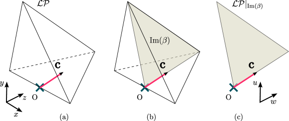
Figure 6: Using symmetry to speed up linear programming: (a) the feasible region of ${\cal LP}$ and the objective vector (in pink); (b) the fixed space of $\mbox{\em Aut}({\cal LP})$ is identified (grey); (c) the feasible region is restricted to its intersection with the fixed space.

To develop lifted linear programming, we proceed as follows: first, we introduce the notion of equitable partitions and show how they connect color-passing. To make use of equitable partitions in linear programs, we need to bridge the combinatorial world of partitions with the algebraic world of linear inequalities. We do so by introducing the notion of fractional automorphisms, which serve as a matrix representation of partitions. Finally, we show that if an LP admits an equitable partition, then an optimal solution of the LP can be found in the span of the corresponding fractional automorphism. This essentially defines our lifting: by restricting the feasible region of the LP to the span of the fractional automorphism, we reduce the dimension of the LP to the rank of the fractional automorphsm (geometric intuition is given in Figure 6). As we will see, this results in an LP with fewer variables (to be precise, we have the same number of variables as the number of classes in the equitable partition).

Now, let us make some necessary remarks on the nature of the partition $\cal U$ returned by Alg. 2. Suppose for now, $\lambda_{0}(e)=1$ for all $e\in E$, i.e. the graph is only vertex-colored. Observe that according to line $8$, nodes $v$ and $v^{\prime}$ receive different colors in the $i$’th iteration if the multisets of the colors of their neighbors are different. That is, in order to be distinguished by Alg. 2, $v$ and $v^{\prime}$ must have a different number of neighbors of the same color at some iteration $i$.

Consequently, as the algorithm terminates when the partition no longer refines, we conclude that the following holds: Alg. 2 partitions a graph $G$ in such a way that every two nodes nodes in the same class have the same number of neighbors from every other class. More formally, for each pair classes $U_{i},U_{j}$ and every two nodes $v,v^{\prime}\in U_{i}$, we have

$$|\operatorname{nb}(v)\cap U_{j}|=|\operatorname{nb}(v^{\prime})\cap U_{j}|\;.$$

We call any partition with the above property equitable. For the edge-colored case, we have a slightly more complicated definition: $\cal U$ is equitable, whenever it holds that for each pair classes $U_{i},U_{j}$, every edge color $c$, and every two nodes $v,v^{\prime}\in U_{i}$

$$|\{w\in U_{j}\ |\ \lambda_{0}(\{v,w\})=c\}|=|\{w^{\prime}\in U_{j}\ |\ \lambda_{0}(\{v^{\prime},w^{\prime}\})=c\}|\;.$$

In other words, we say that every two nodes in a class have the same number of edges of the same color going into every other class.

In fact, it can be shown that Alg. 2 computes the coarsest such partition of a graph, and the relationship between equitable partitions and color-passing has been well-known in graph theory [RSU94].

Observe that like MRFs, which have variables and factors, linear programs are bipartite objects as well: they consists of variables and constraints. As such, they are more naturally represented by bipartite graphs, hence we will now narrow down our discussion to bipartite graphs. We say that a colored graph $G=(V,E,\lambda)$ is biparite, if the vertex set consists of two subsets, $V=A\cup B$, such that every edge in $E$ has one end-point in $A$ and the other in $B$. The notion of equitable partitions apply naturally to the bipartite setting – we will use the notation ${\cal U}=\{P_{1},\ldots,P_{p},Q_{1},\ldots,Q_{q}\}$ to indicate that the classes over the subset $A$ are disjoint from the classes over the subset $B$. I.e., no pair $v\in A,v^{\prime}\in B$ can be in the same equivalence class.

With this in mind, we introduce fractional automorphisms. Note that our definition is slightly modified from the original one [RSU94], in order to accomodate the bipartite setting.

Definition 2.

Let $\bf M$ be an $m\times n$ real matrix, such as the (colored, weighted) adjacency matrix of a bipartite graph. A fractional automorphism of $\bf M$ is a pair of doubly stochastic (meaning that the entries are non-negative, and every row and column sum to one) matrices $\mathbf{X}_{P},\mathbf{X}_{Q}$ such that

$$\mathbf{M}\mathbf{X}_{P}=\mathbf{X}_{Q}\mathbf{M}.$$

The following theorem establishes the correspondence between equitable partitions and fractional automorphisms.

Theorem 3 ([RSU94, GKMS13]).

Let $G$ be a bipartite graph. Then:

• if ${\cal U}=\{P_{1},\ldots,P_{p},Q_{1},\ldots,Q_{q}\}$ is an equitable partition of $G$, then the matrices $\mathbf{X}_{P},\mathbf{X}_{Q}$, having entries

  $$\mathbf{(}X_{P})_{ij}=\begin{cases}1/|P|&\text{ if both vertices }i,\ j\text{ are in the same }P\in{\cal U},\\ 0&\text{ otherwise,}\end{cases}$$

  $$\mathbf{(}X_{Q})_{ij}=\begin{cases}1/|Q|&\text{ if both vertices }i,\ j\text{ are in the same }Q\in{\cal U},\\ 0&\text{ otherwise,}\end{cases}$$ (3)

  is a fractional automorphism of the adjacency matrix of $G$.

• conversely, let $\mathbf{X}_{P},\mathbf{X}_{Q}$ be a fractional automorphism of the (colored, weighted) adjacency matrix of the bipartite $G$ with edge set $V=A\cup B$. Then the partition ${\cal U}$, where vertices $i,j\in A$ belong to the same $P\in{\cal U}$ if and only if at least one of $(\mathbf{X}_{P})_{ij}$ and $(\mathbf{X}_{P})_{ji}$ is greater than $0$, respectively $i,j\in B$ belong to a class $Q$ if $(\mathbf{X}_{Q})_{ij}$ or $(\mathbf{X}_{Q})_{ji}$ is greater than $0$, is an equitable partition of $G$.

In the following, part $i)$ of the above Theorem will be of particular interest to us. We will shortly show how we can use color-passing to construct equitable partitions of linear programs. Encoding these equitable partitions as fractional automorphisms will provides us with insights into the geometrical aspects of lifting and will be an essential tool for proving its soundness.

Note that any graph partition (equitable or not) can be turned into a doubly stochastic matrix using Eq. i). However, keep in mind that the resulting matrix will not be a fractional automorphism unless the partition is equitable. In any case, partition matrices have a useful property that will later on allow us to reduce the number of constraints and variables of a linear program. Namely,

Proposition 4 ([God97]).

Let $\mathbf{X}$ be the doubly stochastic matrix of some partition ${\cal U}$ according to Eq. i). Then $\mathbf{X}=\widetilde{\mathbf{B}}\widetilde{\mathbf{B}}^{T}$, with

$${\widetilde{\bf B}}_{im}=\begin{cases}\frac{1}{\sqrt{|U_{m}|}}&\text{ if vertex }i\text{ belongs to part }U_{m},\\ 0&\text{ otherwise. }\end{cases}$$ (4)

5.3 Fractional Automorphisms of Linear Programs

As we already mentioned, we are going to apply equitable partitions through fractional automorphisms to reduce the size of linear programs. Hence, the obvious question presents itself: what is an equitable partition (resp. fractional automorphism) of linear program?

In order to answer the question, we need a graphical representation of $L=(\mathbf{A},\mathbf{b},\mathbf{c})$, called the coefficient graph of $L$, $G_{L}$. To construct $G_{L}$, we add a vertex to $G_{L}$ for every of the $m$ constraints $n$ variables of $L$. Then, we connect a constraint vertex $i$ and variable vertex $j$ if and only if ${\bf A}_{ij}\neq 0$. Furthermore, we assign colors to the edges $\{i,j\}$ in such a way that $\mbox{\em color}(\{i,j\})=\mbox{\em color}(\{u,v\})\Leftrightarrow{\bf A}_{ij}={\bf A}_{uv}$. Finally, to ensure that $\bf c$ and $\bf b$ are preserved by any automorphism we find, we color the vertices in a similar manner, i.e., for row vertices $i,j$ $\mbox{\em color}(i)=\mbox{\em color}(j)\Leftrightarrow\mathbf{b}_{i}=\mathbf{b}_{j}$ and $color(u)=color(v)\Leftrightarrow{\bf c}_{u}={\bf c}_{v}$ for column vertices. We must also choose the colors in a way that no pair of row and column vertices share the same color; this is always possible.

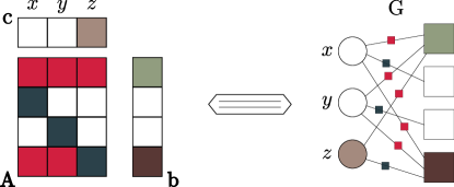
Figure 7: Construction of the coefficient graph $G_{L}$ of $L^{0}$. On the left-hand side, the coloring of the LP is shown. This turns into the colored coefficient graph shown on the right-hand side.

To illustrate this, consider the following toy LP:

⬇

1var p/1;

2

3maximize: sum_{gadget(X)} p(X);

4

5subject to: sum{widget(X)}p(X) + sum{gadget(X)} p(X) <= 1;

6subject to {widget(X)}: widget(X) <= 0;

7subject to: sum{widget(X)}p(X) - sum{gadget(X)} p(X) <= -1;

with knowledge base LogKB (recall that logical atoms are assumed to evaluate to $0$ and $1$ within an RLP):

⬇

widget(x).

widget(y).

gadget(z).

If we ground this linear program and convert it to dual form (as in Eq. 1), we obtain the following linear program $L^{0}=(\mathbf{A},\mathbf{b},\mathbf{c})$

$$\operatorname*{minimize}_{[x,y,z]^{T}\in\mathbb{R}^{3}}\quad \;0x+0y+1z$$

subject to $$\begin{bmatrix}1&1&1\\[3.00003pt] -1&0&0\\[3.00003pt] 0&-1&0\\[3.00003pt] 1&1&-1\\[3.00003pt] \end{bmatrix}\begin{bmatrix}x\\ y\\ z\\ \end{bmatrix}\leq\begin{bmatrix}1\\ 0\\ 0\\ -1\\ \end{bmatrix}\;,$$

where for brevity we have substituted ${\tt p}(x),{\tt p}(y),{\tt p}(z)$ by $x,y,z$ respectively. The coefficient graph of $L^{0}$ is shown in Fig. 7.

We call an equitable partition of a linear program $L$ the equitable partition of the graph $G_{L}$. Suppose now we compute an equitable partition ${\cal U}=\{P_{1},\ldots,P_{p},Q_{1},\ldots,Q_{q}\}$ of $G_{L}$ using Algorithm 2 and compute the corresponding fractinal automorphism $(\mathbf{X}_{P},\mathbf{X}_{Q})$ as in Eq. i). Observer that $(\mathbf{X}_{P},\mathbf{X}_{Q})$ will have the following properties:

• due to Theorem 3, we have $\mathbf{X}_{Q}\mathbf{A}=\mathbf{A}\mathbf{X}_{P}$;

• by our choice of initial colors of $G_{L}$, the partition ${\cal U}$ will never group together variable vertices $i,j$ with $\mathbf{c}_{i}\neq\mathbf{c}_{j}$, nor will it group constraint vertices $i,j$ with $\mathbf{b}_{i}\neq\mathbf{b}_{j}$. By Eq. i), this implies

  $$\mathbf{c}^{T}\mathbf{X}_{P}=\mathbf{c}^{T}$$

  and

  $$\mathbf{X}_{Q}\mathbf{b}=\mathbf{b}\;.$$

This yields the definition of a fractional automorphism of linear programs – we call a pair of doubly stochastic matrices $(\mathbf{X}_{P},\mathbf{X}_{Q})$ a fractional automorphism of the linear program $L$ if it satisfies properties $i)$ and $ii)$ as above.

5.4 Lifted Linear Programming

With this at hand, we are ready for the main part of our argument. We split the argument in two parts: first, we will show that if an LP $L$ has an optimal solution $\mathbf{x}^{*}$, then it also has a solution $\mathbf{X}_{P}\mathbf{x}^{*}$. That is, if we add the constraint $\mathbf{x}\in\operatorname{span}(\mathbf{X}_{P})$ to the linear program, we will not cut away the optimum. The second claim is that $\mathbf{x}\in\operatorname{span}(\mathbf{X}_{P})$ can be realized by a projection of the LP into a lower dimensional space. So, we can actually project to a low-dimensional space, solve the LP there, and then recover the high-dimensional solution via simple matrix multiplication. We recall that his idea is illustrated in Figure 6.

Let us now state the main result.

Theorem 5.

Let $L=(\mathbf{A},\mathbf{b},\mathbf{c})$ be a linear program and $(\mathbf{X}_{P},\mathbf{X}_{Q})$ be a fractional automorphism of $L$. Then, it holds that if $\mathbf{x}$ is a feasible in $L$, then $\mathbf{X}_{P}\mathbf{x}$ is feasible as well and both have the same objective value. As a consequence, if $\mathbf{x}^{*}$ is an optimal solution, $\mathbf{X}_{P}\mathbf{x}^{*}$ is optimal as well.

Proof.

Let $\mathbf{x}$ be feasible in $L=(\mathbf{A},\mathbf{b},\mathbf{c})$, i.e. $\mathbf{A}\mathbf{x}\leq\mathbf{b}$. Observe that left multiplication of the system by a doubly stochastic matrix preserves the direction of inequalities. More precisely

$$\mathbf{A}\mathbf{x}\leq\mathbf{b}\Rightarrow\mathbf{S}\mathbf{A}\mathbf{x}\leq\mathbf{S}\mathbf{b}\;,$$

for any doubly stochastic $\mathbf{S}$. So now, we left-multiply the system by $\mathbf{X}_{Q}$:

$$\mathbf{A}\mathbf{x}\leq\mathbf{b}\Rightarrow\mathbf{X}_{Q}\mathbf{A}\mathbf{x}\leq\mathbf{X}_{Q}\mathbf{b}=\mathbf{A}\mathbf{X}_{P}\mathbf{x}\leq\mathbf{b},$$

since $\mathbf{X}_{Q}\mathbf{A}=\mathbf{A}\mathbf{X}_{P}$ and $\mathbf{X}_{Q}\mathbf{b}=\mathbf{b}$. This proves the first part of our Theorem. Finally, observe that $\mathbf{c}^{T}(\mathbf{X}_{P}\mathbf{x})=\mathbf{c}^{T}\mathbf{x}$ as $\mathbf{c}^{T}\mathbf{X}_{P}=\mathbf{c}^{T}$. $\Box$

We have thus shown that if we add the constraint $\mathbf{x}\in\operatorname{span}(\mathbf{X}_{P})$ to $L$, we can still find a solution of the same quality as in the original program. How does this help to reduce dimensionality? To answer, we observe that the constraint $\mathbf{x}\in\operatorname{span}(\mathbf{X}_{P})$ can be implemented implicitly, through reparametrization. That is, instead of adding it to $L=(\mathbf{A},\mathbf{b},\mathbf{c})$ explicitly, we take the LP $L^{\prime}=(\mathbf{A}\mathbf{X}_{P},\mathbf{b},\mathbf{X}_{P}^{T}\mathbf{c})$. Now, recall that $X_{P}$ was generated by an equitable partition, and it can be factorized as $X_{P}=\widetilde{\mathbf{B}}_{P}\widetilde{\mathbf{B}}_{P}^{T}$ where $\widetilde{\mathbf{B}}_{P}$ is the normalized incidence matrix of $\{P_{1},\ldots,P_{p}\}\subset{\cal U}$ as in Eq. 4.

Note that the span of $\mathbf{X}_{P}=\widetilde{\bf B}_{P}\widetilde{\bf B}_{P}^{T}$ is equivalent (in the vector space isomorphism sense) to the column space of $\widetilde{\bf B}_{P}$. That is, every $\mathbf{x}\in\mathbb{R}^{n}$, $\mathbf{x}\in\operatorname{span}(\mathbf{X}_{P})$ can be expressed as $\mathbf{x}=\widetilde{\bf B}_{P}\mathbf{y}$ some $y\in\mathbb{R}^{p}$ and conversely, $\widetilde{\bf B}_{P}\mathbf{y}\in\operatorname{span}(\mathbf{X}_{P})$ for all $\mathbf{y}\in\mathbb{R}^{p}$.Hence, we can replace $L^{\prime}=(\mathbf{A}\mathbf{X}_{P},\mathbf{b},\mathbf{X}_{P}^{T}\mathbf{c})$ with the equivalent $L^{\prime\prime}=(\mathbf{A}\widetilde{\bf B}_{P},\mathbf{b},\widetilde{\bf B}^{T}_{P}\mathbf{c})$ . Since this is now a problem in $p\leq n$ variables, i.e., of reduced dimension, a speed-up of solving the original LP is possible. Finally, by the above, if $\mathbf{y}^{*}$ is an optimal solution of $L^{\prime\prime}$, $\widetilde{\bf B}_{P}\mathbf{y}$ is an optimum solution of $L$.

Input: An inequality-constrained LP, $L=(\mathbf{A},\mathbf{b},\mathbf{c})$

Output: $\mathbf{x}^{*}=\operatornamewithlimits{argmin}_{\{\mathbf{x}|\mathbf{Ax}\leq\mathbf{b}\}}{\mathbf{c}^{T}\mathbf{x}}$

1 Construct the coefficient graph $G_{L}$;

2 Lift $G_{L}$ using color-passing, see Alg. 2.;

3 Read off the characteristic matrix $\widetilde{\mathbf{B}}_{P}$;

4 Obtain the solution $\mathbf{y}$ of the LP $(\mathbf{A}\widetilde{\mathbf{B}}_{P},\mathbf{b},\widetilde{\mathbf{B}}_{P}^{T}\mathbf{c})$ using any standard LP solver;

5 return $\mathbf{x}^{*}=\widetilde{\mathbf{B}}_{P}\mathbf{y}$;

Algorithm 3 Lifted Linear Programming

Overall, this yields the lifted linear programming approach as summarized in Alg. 3. Given an LP, first construct the coefficient graph of the LP (line 1). Then, lift the coefficent graph (line 2) and read off the characteristic matrix (line 3). Solve the lifted LP (line 4) and “unlift” the lifted solution to a solution of the original LP (line 5).

Applying this lifted linear programming to LPs induced by RLPs, we can rephrase relational linear programming as follows:

1. Specify an RLP $R$.

2. Given a LogKB, ground $R$ into an LP $L$ (Alg. 1).

3. Solve $L$ using lifted linear programming (Alg. 3).

Before illustrating relational linear programming, we would like to note that this method of constructing fractional automorphisms works for any equitable partition, not only the one resulting from running color-passing. For example, an equitable partition of a graph can be constructed out of its automorphism group, by making two vertices equivalent whenever there exists a graph automorphism that maps one to the other. The resulting partition is called the orbit partition of a graph, see e.g. [GR01]. Applying this partitioning method to coefficient graphs of linear programs and using the corresponding fractional automorphism is equivalent to previous theoretical well-known results in solving linear programs under symmetry, see e.g. [BHJ13] and references in there. However, there are two major benefits for using the color-passing partition instead of the orbit partition:

• The color-passing partition is at least as coarse as the orbit partition, see e.g. [GR01]. To illustrate this, consider the so-called Frucht graph as shown in Fig. 8. Suppose we turn this graph into a linear program by introducing constraint nodes along the edges and coloring everything with the same color. The Frucht graph has two extreme properties with respect to equitable partitions: 1) it is asymmetric, meaning that the orbit partition is trivial – one vertex per equivalence class; 2) it is regular (every vertex has degree 3); as one can easily verify, in this case the coarsest equitable partition consists of a single class!

  

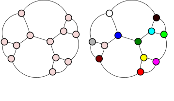
  Figure 8: The Frucht graph with 12 nodes. The colors indicate the resulting node partitions using color-passing (the coarsest equitable partition, eft) and using automorphisms (the orbit partition, right).

  Due to these two properties, in the case of the Frucht graph the orbit partition yields no compression, whereas the coarsest equitable resp. color-passing partition produces an LP with a single variable.

• The color-passing partition can be computed in quasi-linear time [BBG13], yet current tools for orbit partition enumeration have significantly worse running times. Thus, by using color-passing we achieve strict gains in both compression and efficiency compared to using orbits.

Let us now illustrate relational linear programming using several AI tasks.

6 Illustrations of Relational Linear Programming

Our intention here is to investigate the viability of the ideas and concepts of relational linear programming through the following questions:

(Q1)

Can important AI tasks be encoded in a concise and readable relational way using RLPs?

(Q2)

Are there (R)LPs that can be solved more efficiently using lifting?

(Q3)

Does relational linear programming enable a programming approach to AI tasks facilitating the construction of more sophisticated models from simpler ones by adding rules?

If so, relational linear programming has the potentially to make linear models faster to write and easier to understand, reduce the development time and cost to encourage experimentation, and in turn reduce the level of expertise necessary to build AI applications. Consequently, our primary focus is not to achieve the best performance by using advanced models. Instead we will focus on basic models.

We have implemented a prototype system of relational linear programming, and illustrate the relational modeling of several AI tasks: computing the value function of Markov decision processes, performing MAP LP inference in Markov logic networks and performing collective transductive classification using LP support vector machines.

6.1 Lifted Linear Programming for Solving Markov Decision Processes

Our first application for illustrating relational linear programing is the computation of the value function of Markov Decision Problems (MDPs). The LP formulation of this task is as follows [LDK95]:

$$\operatorname*{maximize}\nolimits_{\mathbf{v}} \mathbf{1}^{T}\mathbf{v},$$

subject to $$\ v_{i}\leq c_{i}^{k}+\gamma\sum\nolimits_{j\in\Omega_{S}}p_{ij}^{k}v_{j}\;,$$ (5)

where $v_{i}$ is the value of state $i$, $c_{i}^{k}$ is the reward that the agent receives when carrying out action $k$, and $p_{ij}^{k}$ is the probability of transferring from state $i$ to state $j$ by taking action $k$. $\gamma$ is a discounting factor. The corresponding RLP is given in Fig. 9. Since it abstract away the states and rewards — they are defined in the LogKB — it extracts the essence of computing value functions of MDPs. Given a LogKB, a ground LP is automatically created Instead of coding the LP by hand for each problem instance again and again as in vanilla linear programming. This answers question (Q1) affirmatively.

⬇

1var value/1; #value function to be determined by the LP solver

2

3maximize: sum{reward(S,_)} value(S); #best values for all states

4

5#encoding of discounted Bellman optimality as in inequality (5)

6subject to {transProb(S,T,_)}: value(S) <= reward(S,A) +

7 gamma*sum{transProb(S,T,A)} transProb(S,T,A)*value(T);

Figure 9: An RLP for computing the value function value/1 of a Markov decision process. There is a finite set of states and actions, and the agent receives a reward reward(S,A) for performing and action A in state S, specified in a LogKB.

The MDP instance that we used is the well-known Gridworld (see e.g. [SB98]). The gridworld problem consists of an agent navigating within a grid of $n\times n$ states. Every state has an associated reward $R(s)$. Typically there is one or several states with high rewards, considered the goals, whereas the other states have zero or negative associated rewards. We considered an instance of gridworld with a single goal state in the upper-right corner with a reward of $100$. The reward of all other states was set to $-1$. The scheme for the LogKB looked like this:

⬇

reward(state(n-1,n),right)=100.

reward(state(n,n-1),up)=100.

reward(state(X,Y),_)=-1 :- X>0, X<n-1, Y>0, Y<n-1.

As can be seen in Fig. 10(a), this example can be compiled to about half the original size. Fig. 10(b) shows that already this compression leads to improved running time. We now introduce additional symmetries by putting a goal in every corner of the grid. As one might expect this additional symmetry gives more room for compression, which further improves efficiency as reflected in Figs. 10(c) and  10(d).

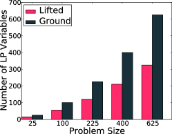
(a) Ground vs. lifted variables on a basic gridworld MDP.

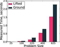
(b) Measured times on a basic gridworld MDP.

(c) Variables on a gridworld with additional symmetry.

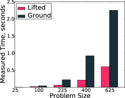
(d) Measured times on a gridworld with additional symmetry.

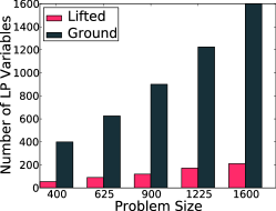
(e) Variables on a gridworld with additional symmetry in sparse form.

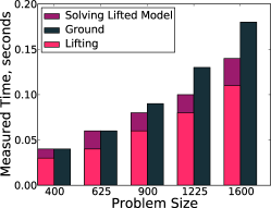
(f) Measured times on a gridworld with additional symmetry in sparse form.

Figure 10: Experimental results of relational linear programming for solving Markov decision processes.

However, the examples that we have considered so far are quite sparse in their structure. Thus, one might wonder whether the demonstrated benefit is achieved only because we are solving sparse problem in dense form. To address this we convert the MDP problem to a sparse representation for our further experiments. We scaled the number of states up to $1600$ and as one can see in Fig. 10(e) and (f) lifting still results in an improvement of size as well as running time. Therefore, we can conclude that lifting an LP is beneficial regardless of whether the problem is sparse or dense, thus one might view symmetry as a dimension orthogonal to sparsity. Furthermore, in Fig. 10(f) we break down the measured total time for solving the LP into the time spent on lifting and solving respectively. This presentation exposes the fact that the time for lifting dominates the overall computation time. Clearly, if lifting was carried out in every iteration (CVXOPT took on average around 10 iterations on these problems) the approach would not have been competitive to simply solving on the ground level. This justifies that the loss of potential lifting we had to accept in order to not carry out the lifting in every iteration indeed pays off (Q2). Remarkably, these results follow closely what has been achieved with MDP-specific symmetry-finding and model minimization approaches [NR08, RB01, DG97].

6.2 Programming MAP LP Inference in Markov Logic Networks

⬇

1var m/2; #single node, pairwise, and

2var m/4; #triplewise probabilities

3var m/6; #of configurations to be determined by the solver

4#value of the MAP assignment

5innerProd = sum{w(P, V)} w(P, V) * m(P, V) +

6 sum{w(P1, P2, V1, V2)} w(P1, P2, V1, V2) * m(P1, P2, V1, V2) +

7 sum{w(P1, P2, P3, V1, V2, V3)} w(P1, P2, P3, V1, V2, V3) *

8 m(P1, P2, P3, V1, V2, V3);

9atomMarg(P) = sum {w(P, V)} m(P, V); #single node marginals

10#single node marginal computed from pairwise marginals

11clauseMargl1(P1, P2, V1) = sum{w(P2, V2)} m(P1, P2, V1, V2);

12...

13#single node marginal computed from triplewise marginales

14clauseMarg1(P1, P2, P3, V1) = sum{w(P3, V3), w(P2, V2)}

15 m(P1, P2, P3, V1, V2, V3);

16...

17maximise: innerProd; #find MAP assignment with largest value

18

19subject to {w(P, _)}: atomMarg(P) = 1; #normalization constraint

20#pairwise consistency constraints

21subject to {w(P1, P2, V1, _)}: m(P1, V1) - clauseMarg1(P1, P2, V1) = 0;

22...

23#triplewise consistency constraints

24subject to {w(P1, P2, P3, V1, _, _)}:

25 m(P1, V1) - clauseMarg1(P1, P2, P3, V1) = 0;

26...

Figure 11: RLP encoding the MAP-LP for triplewise MLNs as shown in Eq. 6. The last two constraints as well as the last two aggregates have symmetric copies that have been omitted (this redundancy is necessary, since logic predicates are not symmetric).

MLNs, see  [RD06] for more details, are a prominent model in statistical relational learning (SRL). We here focus on MAP (maximum a posteriori) inference where we want to find a most likely joint assignment to all the random variables. More precisely, an MLN induces a Markov random field (MRF) with a node for each ground atom and a clique for every ground formula. A common approach to approximate MAP inference in MRFs is based on LP, see e.g. [WJ08] for a general overview. Actually, there is a hierarchy of LP formulation for MAP inference each assuming a hypertree MRF of increasing treewidth. Since MLNs of interest typically consists of at least one factor with three random variables, we will focus on triplewise MRFs as presented e.g. in [AKM14] in order to investigate (Q1). Given an MRF $\mathcal{M}$ induced by an MLN over the set of (ground) random variables $x=\{x_{i},\ldots,x_{n}\}$ and with factors $F=\{(\theta_{f},x_{f})\}_{f}$, the MAP-LP is define as follows, see also [AKM14]. For each subset of indices $\mathcal{I}$ taken from $\{1,\ldots,n\}$ of size $1\leq|\mathcal{I}|\leq 3$, let $\mu_{\mathcal{I}}$ denote a vector of variables of size $2^{|\mathcal{I}|}$. A notation $\mu_{ijk}(x_{i},x_{j},x_{k})$ is used to describe a specific variable in vector $\mu_{\mathcal{I}}$ corresponding to the subset $\mathcal{I}=(i,j,k)$ and entry $(x_{i},x_{j},x_{k})\in{\{0,1\}}^{3}$. Additionally, let $\mathcal{I}_{F}$ denote the set of all ordered indices for which there exists a factor $f$ with a matching variables scope $x_{f}$, and let $\theta_{ijk}$ denote the log probability table of a factor whose variables scope is $(x_{i},x_{j},x_{k})$. The MAP-LP is now defined as follows:

$$\text{maximize}_{\mu}\sum_{(i)\in\mathcal{I}_{F}}\langle\theta_{i},\mu_{i}\rangle+\sum_{(i,j)\in\mathcal{I}_{F}}\langle\theta_{ij},\mu_{ij}\rangle+\sum_{(i,j,k)\in\mathcal{I}_{F}}\langle\theta_{ijk},\mu_{ijk}\rangle$$ (6)

$$\begin{tabular}[]{ >{$}l<{$} >{$}l<{$} >{$}l<{$} >{$}l<{$}}\text{subject to }&\sum_{x_{i}}\mu_{i}(x_{i})=1&\forall(i)\in\mathcal{I}_{F},&\\ &\sum_{x_{j}}\mu_{ij}(x_{i},x_{j})=\mu_{i}(x_{i})&\forall(i,j)\in\mathcal{I}_{F},&\\ &\sum_{x_{i}}\mu_{ij}(x_{i},x_{j})=\mu_{j}(x_{j})&\\ &\mu_{ijk}(x_{i},x_{j},x_{k})\geq 0&\forall(i,j,k)\in\mathcal{I}_{F},&\\ &\sum_{x_{k}}\mu_{ijk}(x_{i},x_{j},x_{k})=\mu_{ij}(x_{i},x_{j})&\\ &\sum_{x_{j}}\mu_{ijk}(x_{i},x_{j},x_{k})=\mu_{ik}(x_{i},x_{k})&\\ &\sum_{x_{i}}\mu_{ijk}(x_{i},x_{j},x_{k})=\mu_{jk}(x_{j},x_{k})&\end{tabular}\$$

$$\text{where }\langle\theta_{ijk},\mu_{ijk}\rangle=\sum_{(x_{i},x_{j},x_{k})}\theta_{ijk}(x_{i},x_{j},x_{k})\cdot\mu_{ijk}(x_{i},x_{j},x_{k})$$

This MAP-LP has to be instantiated for each MLN after we have computed a ground MRF induced by the MLN and a set of constants.

The fact that both MLNs and RLPs are based on logic programming features a different and more convenient translation from an MLN to a MAP LP for inference. Actually, each MAP-LP is defined through weights, marginals, and triples of variables induced by the MLN formulas. This generation can naturally be specified at the lifted level as done in the RLP in Fig. 11. Since it is defined at the lifted level abstracting from the specific MLN, it clearly answers (Q1) affirmatively. To see this, consider to perform inference in the well known smokers MLN. Here, there are two rules. The first rule says that smoking can cause cancer

$$0.75\ \mathtt{smokes(X)\ \operatorname{:-}\ cancer(X)},$$

and the second implies that if two people are friends then they are likely to have the same smoking habits

$$0.75\ \mathtt{smokes(X)\ \operatorname{:-}\ friends(X,Y),smokes(X)}.$$

Since the second formula contains three predicates using the triplewise MAP-LP is valid. Now the the MLN as well as the used constants are encoded in the following LogKB:

⬇

person(anna). person(bob). ... #the people in the social network

value(0). value(1). #we consider binary MLNs

#encoding of the MLN clauses and their weights

w(smokes(X), cancer(X), 1, 0) = 0 :- person(X).

w(smokes(X), cancer(X), V1, V2) = 0.75 :-

person(X), value(V1), value(V2).

w(friends(X, Y), smokes(X), smokes(Y), 1, 1, 1) = 0.75 :-

person(X), person(Y).

w(friends(X, Y), smokes(X), smokes(Y), 1, 0, 0) = 0.75 :-

person(X), person(Y).

w(friends(X, Y), smokes(X), smokes(Y), V1, V2, V3) = 0 :-

person(X), person(Y), value(V1), value(V2), value(V3).

m(smokes(gary), 1). #the smokers we know

m(smokes(helen), 1).

m(friends(anna, bob), 1). #the observed friendship relations

...

m(friends(helen,iris), 1).

This examples gives us an opportunity to introduce another benefit of mixing logic with arithmetics, namely the ability to easily represent such concepts as indicator functions. In the MAP LP we can add an ”indicator” predicate clause(X, Y) which equals to 1 if X and Y are two atoms that form a clause in an MLN and is 0 otherwise. This results in the following extension to the LogKB:

⬇

clause(smokes(X), cancer(X)) = 1 :- person(X).

We can now write the LP constraints in a more mathematical way using constraints such as

⬇

1subject to: {pred(P1), pred(P2), val(V2)}

2 (m(P2,V2) - clauseMarg2(P1,P2,V2))*clause(P1, P2) = 0;

The resulting program is equivalent to the previous version, but can be more straightforward for some people with an optimization background. Both programs show that MAP-LP inference within MLNs can be compactly represented as an RLP. Only the LogKB changes when the MLN and/or the evidence changes. Moreover, the RLP does not rely on the fact that we consider MLNs. Propositional models can be encoded in the LogKB, too. Hence the RLP extracts the essence of MAP-LP inference in probabilistic models, whether relational or propositional. This supports even more that (Q1) can be answered affirmatively.

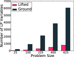
(a) Number of variables in the lifted and ground LPs.

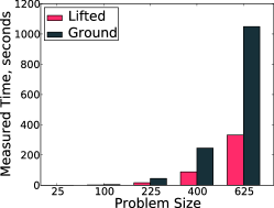
(b) Time for solving the ground LP vs. time for lifting and solving.

Figure 12: Experimental results of relational linear programming for MAP-LP inference within Markov logic networks.

Let us now turn towards investigating Q2. As shown in previous works, inference in graphical models can be dramatically sped-up using lifted inference. Thus, it is natural to expect that the symmetries in graphical models which can be exploited by standard lifted inference techniques will also be reflected in the corresponding MAP-(R)LP. To verify whether this is indeed the case we induced MRFs of varying size from a pairwise smokers MLN [FKD⁺12]. In turn, we used a pairwise MAP-RLP following essentially the same structure as the triplewise MAP-RLP above but restricted to pairs. We scaled the number of random variables from $25$ to $625$ arranged in a grid with pairwise and singleton factors with identical potentials. The results of the experiments can be seen in Figs. 12(a) and (b). As Fig. 12(a) shows, the number of LP variables is significantly reduced. Not only is the linear program reduced, but due to the fact that the lifting is carried out only once, we also measure a considerable decrease in running time as depicted in Fig. 12(b). Note that the time for the lifted experiment includes the time needed to compile the LP. This affirmatively answers (Q2).

6.3 Programming Collective Classification using LP-SVM

Networks have become ubiquitous, and often we are interested in how objects in these networks influence each other. Consequently, collective classification has received a lot of attention recently [CDI98, NJ00, NJ03, NJ07, RD06, SNB⁺08a]. It refers to the task of jointly classifying a set of inter-related objects. It exploits the fact that inter-related objects often share a lot of similarities. For example, in citation networks there are dependencies among the topics of a papers’ references, and in social networks people who are in a close contact tend to have similar interests. Using these dependencies instead of trying to fight them allows collective classification methods to outperform methods that assume object independence [CDI98].

Despite being successful, most of the research in collective classification so far has focused on generative models, at least as part of column generation approach to solving quadratic program formulations of the collective classification task. We here illustrate that relational linear programming could provide a first step towards a principled large-margin approach. Specifically, we introduce a transductive collective SVM based on RLPs. That is, since we observe a class label for a number of objects resp. instances, say, the topics of papers and we have information about relationships among instances, say the citations among papers, we predict the topics of related but unlabeled papers based on the relationship to the observed ones and, possibly, some other attributes.

More precisely, we seek the largest separation between labeled and unlabeled nodes through regularization within a relational linear program approximation to SVMs. We start off by reviewing the vanilla LP approach to SVMs and then show how RLPs can be used to program a transductive collective classifier.

⬇

1var slack/1; #the slacks

2var weight/1; #the slope of the hyperplane

3var b/0; #the intercept of the hyperplane

4var r/0; #margin

5

6slacks=sum{label(I)} slack(I); #total slack

7innerProd(I)=sum{attribute(_,J)} weight(J)*attribute(I,J); #hyperplane

8

9#find the largest margin. Here const encodes a trade-off parameter

10minimize: -r + const * slacks;

11

12#examples should be on the correct side of the hyperplane

13subject to {label(I)}: label(I)*(innerProd(I) + b) + slack(I) >= r;

14#weights are between 0 and 1

15subject to {attribute(_, J)}: -1 <= weight(J) <= 1;

16subject to : r >= 0; #the margin is positive

17subject to {label(I)}: slack(I) >= 0; #slacks are positive

Figure 13: A linear programming SVM encoded as an RLP. Note, for convenience, we now use a minimize instead of a maximize statement.

Support vector machines (SVMs) [Vap98] are the most widely used model for discriminative classification at the moment. SVMs’ hypothesis space is the space of linear models over numeric attributes of the data. Training is done by minimizing the number of misclassified examples and maximizing the gap between correctly classified examples and the separating hyperplane, with the squared norm of the weight vector as a normalization factor. This task is traditionally posed as a quadratic optimization problem (QP). Zhou et. al. [ZZJ02] have shown that the same problem can be modeled as an LP with only a small loss in generalization performance. The LP they suggested is the following:

$$\operatorname{minimize}\quad \;-r+C\sum\nolimits_{i=1}^{l}\xi_{i}$$

subject to $$\;y_{i}(\mathbf{w}\mathbf{x}_{i}+b)\geq r-\xi_{i}\;,$$

$$-1\leq\mathbf{w}_{i}\leq 1\;,$$

$$\xi_{i}\geq 0\;,$$

$$r\geq 0\;,$$

and we refer to [ZZJ02] for more details. This LP-SVM can readily be applied to classify papers in the Cora dataset [SNB⁺08b]. The Cora dataset consists of $2708$ scientific publications classified into one of seven classes. The citation network consists of 5429 links. Each publication in the dataset is described by a 0/1-valued word vector indicating the absence/presence of the corresponding word from the dictionary. The dictionary consists of $1433$ unique words. We turned this problem into a binary classification problem by taking the most common of $7$ classes as a positive class and merging the other $6$ into a negative class.

To do so, we have to provide the RLP and the corresponding LogKB. The RLP in Fig. 13 encodes the the vanialla LP-SVM. Since it is not collective, we completely ignored the citation information and classified documents based on 0/1 word features using the following LogKB:

⬇

const = 0.021.

attribute(31336, 119). attribute(31336, 126). ...

label(17798) = -1. label(10531) = 1. ...

Here the arguments of the attribute/2 predicate are indices of a document and a word present in a document respectively. Words that are not present in a document, i.e., they have value zero in the original dataset, are not specified. Again, this answers (Q1) affirmatively, since the RLP stays fix for different datasets.

We now show how to transform this vanilla (R)LP-SVM model into a transductive collective one (TC-RLP-SVM) just by programming.

Indeed, there are a number of ways to do this. We chose the following approach. We added constraints which ensure that unlabeled instances have the same label as the labeled ones to which they are connected by a citation relation. To account for contradicting examples, in the spirit of SVMs, we introduced slack variables for these constraints and added them to the objective with a separate parameter. This resulted in the changes to the RLP-SVM shown in Fig. 14. Here, the new predicate pred/2 denotes the predicted label for unlabeled instances. The LogKB gets two new predicates:

⬇

const(1) = 0.0021. const(2) = 0.0031.

cite(89547, 1132385). cite(89547, 1152379). ...

query(1128959). query(16008). ...

⬇

1var pred/1; #predicted label for unlabeled instances

2var slack/2; #slack between neighboring instances

3...

4slacks1 = sum{label(I)} slack(I); #total label slack

5slacks2 = sum{label(I1,l2)} slack(I1,l1); #total inter-label slack

6#find the largest margin. Here the consts encode trade-off parameters

7minimize: -r + const(1) * slacks1 + const(2) * slacks2;

8...

9#examples should be on the correct side of the hyperplane

10subject to {query(I)}: pred(I) = innerProd(I) + b;

11#related instances should have the same labels.

12subject to {cite(I1, I2), label(I1), query(I2)}:

13 label(I1) * pred(I2) + slack(I1, I2) >= r;

14#the symmetric case

15subject to {cite(I1, I2), label(I2), query(I1)}:

16 label(I2) * pred(I1) + slack(I1, I2) >= r;

Figure 14: An RLP-SVM model for collective inference in a transductive setting. Shown are only the changes and add-ons to the vanilla RLP-SVM model from Fig. 13.

The cite/2 predicate represent citation information, and the query predicate marks unlabelled instances whose labels are to be inferred. We notice that the parameters in the objective play a radically different role in the TC-RLP-SVM. In the vanilla case a parameter has to be carefully chosen on the training phase, but then prediction is done using the learned weight vector only. In the transductive setting the linear model, which is in the heart of RLP-SVM, plays a role of a media between labeled and unlabeled instances. The weights are tuned for every new problem instance (remember, that the whole point of transductive inference is not to learn an intermediate predictive model, but to do inference directly). In this case the objective parameters become a lot more important. In turns out that the optimal value of the parameters depends on the size of a problem and hence they have to be tuned during the transductive inference phase as well using e.g. cross-validation.

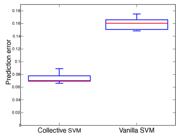
(a) Box plot for prediction errors of collective and vanilla SVMs using RLPs.

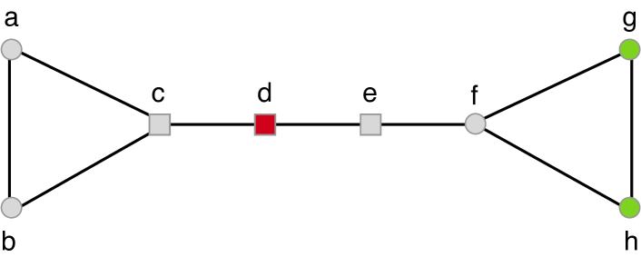
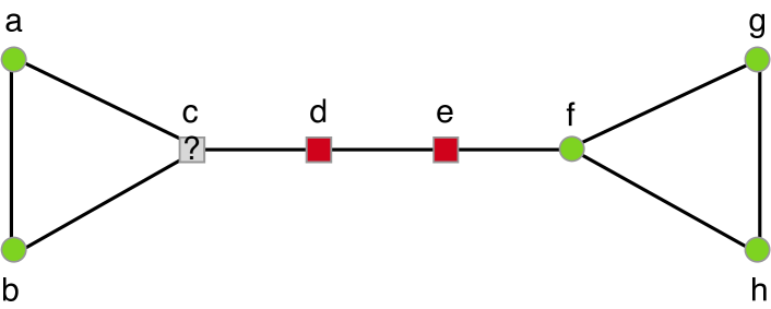
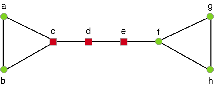
(b) Lifted solving RLP-SVMs.

Figure 15: Experimental results of linear programming support vector machines. (a) TC-RLP-SVM (left) versus vanilla RLP-SVM on the CORA dataset. (b) Liifted RLP-SVM experiments. (Top) Training set. Nodes can have different shapes and different degrees. The task is to predict the colors red resp. green for the gray nodes. (Middle) predictions of the vanilla RLP. The ‘?’ indicates that the SVM cannot make a definite prediction. (Bottom) Predictions of the TC-RLP-SVM. In both cases the induced LPs were solved using lifted linear programming

To illustrate the benefit of the TC-RLP-SVM we compared its performance with that of the vanilla RLP-SVM on the task of paper topic classification in the Cora dataset. The experiment protocol was as follows. We first randomly split the dataset into a training set $A$, a validation set $C$, and a test set $B$ in proportion $70/15/15$. The validation set was used to select the parameters of the TC-RLP-SVM in a $5$-fold cross-validation fashion. That is, we split the validation set into $5$ subsets $C_{i}$ of equal size. On these sets we performed parameter selection by doing a grid search for each $C_{i}$ on a $A\cup(C\setminus C_{i})$ labeled and $B\cup C_{i}$ unlabeled examples, computing the prediction error on $C_{i}$ and averaging it over all $C_{i}$s. We then evaluate the selected parameters on the test set $B$ whose labels were never revealed in training. We repeat this experiment $5$ times, one for each $C_{i}$, for both the TC-RLP-SVM and the vanilla RLP-SVM. The results are summarized in Fig. 15a. The vanilla RLP-SVM achieved a prediction error of $16\pm 1\%$. The TC-RLP-SVM achieved $7.5\pm 1\%$. A paired t-test ($p=0.05$) revealed that the difference in mean is significant. Although best performance was not our goal, the performance is quite encouraging. For instance, Klein et al. [KBS08] reported error rates of about $13\%$ for there structured SVM although using different folds. In any case, just reprogramming the RLP-SVM — adding three relational constraints — resulted in a $50\%$ error reduction. This clearly answers (Q3) affirmatively.

6.4 Lifted Solving Relational Linear Programming Support Vector Machines

Finally, to close the loop, we illustrate that RLP-SVMs are liftable, too. Although not surprising from a theoretical perspective — we have already shown that any LP that contains symmetries is liftable — this constitutes the very first symmetry-aware SVM solver and is an encouraging sign that lifting goes beyond probabilistic inference, i.e., lifted statistical machine learning may not be insurmountable.

The problem we considered is the one of predicting the color (red/green) of a vertex in an extended version of the so called McKay graph as shown in Fig. 15b(top). The only attributes used for classification are the degree of a vertex and its shape (circle or square). Gray nodes are unlabeled. This resulted in the following LogKB for the TC-RLP-SVM:

⬇

edge(a, b). ... edge(h, g).

label(f) = 1. label(g) = 1. label(d) = -1.

sim_edge(X, Y) :- edge(X, Y).

sim_edge(X, Y) :- edge(Y, X).

attribute(a, shape) = 1. ... attribute(h, shape) = 1.

and the following additional definition in the RLP:

⬇

attribute(X, degree) :- sum <sim_edge(X, _)> 1;

Due to the model/instance separation property of RLPs we can directly apply the vanilla RLP-SVM from Fig. 13. This resulted in the color predictions shown in Fig. 15b(middle). As one can clearly see, the vanilla LP-SVM can predict correctly colors for nodes a, b ,e and f, but fails to predict a color for the node c ( it gives 0 prediction).

Then, we added the same collective constraints we used already in the RLP shown in Fig. 14. That is, we constraint uncolored nodes to have the same color as their colored neighbors where possible). Using this neighborhood information allowed the collective LP-SVM to correctly classify all the nodes in the graph as show in Fig. 15b(bottom). The reason seems to be that the vanilla RLP-SVM uses both degree and color attributes whereas the collective RLP-SVM can set the degree weight to zero due to the additional constraints and, hence, makes predictions based only on the shape attribute, which is enough to achieve a perfect classification on this graph.

More interestingly, in both cases there is lifting, i.e., the dimensions of the (induced) LP-SVMs were reduced. More precisely, the RLP-SVM was reduced from $46$ variables and constraints down to $22$, only $48\%$ of the original size. The collective version was compressed even slightly more, namely from $63$ down to $29$. This is $46\%$ of the original size. Most interestingly, the lifted collective RLP-SVM is of smaller size than the original vanilla LP-SVM. This supports an affirmative answers of (Q2).

Taking all results together, the illustrations clearly show that all three questions (Q1) – (Q3) can be answered affirmatively.

7 Future work

Relational linear programming is attractive for many AI and machine learning problems, but much remains to be done. For instance, the language could be extended with the concepts of modules and name spaces, allowing one to build libraries of relational programs, as well as combining it with Mattingley and Boyd’s [MB12] CVXGEN to automatically generate custom C code that compiles into a reliable, high speed solver for the problem family at hand. The framework should also be extended to other mathematical programs such as integer LPs, mixed integer programs, quadratic programs, and semi-definite programs, among others. Together with the declarative nature of this relational mathematical programming approach to AI, one should investigate program analysis approaches to automate problem decomposition at a lifted level. If symmetries could be detected and exploited efficiently in other mathematical program families, too, this would put general symmetry-aware machine learning and AI even more into reach. It would also be interesting to investigate infinite relational linear programs.

The most attractive immediate avenue, however, is to explore relational linear programming within AI and machine learning tasks. First of all, the novel collective classification approach should be rigorously be evaluated and compared to other approaches on a number of other benchmark datasets. Other attractive avenues are the exploration of the symmetry-aware SVMs outlined in the present paper within other learning setting, relational dimensionality reduction via LP-SVMs [BBE⁺03], novel relational boosting approaches via linear programs [DBS02], and developing relational and lifted solvers for computing optimal Stackelberg strategies in two-player normal-form game [CS06], among others. One should also push the programming view on relational machine learning tasks. As a prominent example consider kernels for classifying graphs. Graphs classification is a very important task in bioinformatics [APB⁺08], natural language processing [SHSM03] and many other fields. Kernelised SVM is often the method of choice. The idea is to represent an SVM optimization objective in such a way that instance vectors only appear in inner products with each other. These inner products can then be replaced by functions (kernels) that effectively represent inner products in higher dimensional space. This inner product view on one hand makes SVM a non-linear classifier but also allows one to deal with structured objects such as graphs e.g. using convolution kernels [Hau99]. Convolutions kernels introduced the idea that kernels could be built to work with discrete data structures interactively from kernels for smaller composite parts. RLPs suggests to view them as a programming task. Within the logical knowledge base we define the parts and a generalized sum over products — a generalized convolution — is realized within the relational mathematical program. Similarly, many other graph kernels known could be realized. Walks [Gär02], cyclic patterns [HGW04] and shortest-paths [BK05] are examples of substructures considered so far. One can easily see that all these concepts are naturally representable as a logic programs in Prolog. Assume e.g. that $\mathtt{shortestPath(A,B,G,Paths)}$ computes in Path the shortest path between nodes A and B in graph G For instance, we can program the shortest path in Prolog as follows: We can then use it to define the convolution kernel in an RLP SVM as follows:

⬇

1k(G1, G2) = sum{vertex(G1,V1), vertex(G1,V2),

2 shortestPath(V1,V2,G1,L1), vertex(G2,V3), vertex(G2,V4),

3 shortestPath(V3,V4,G2,L2)}

4 simple_k(V1,V2,L1,V3,V4,L2).

5simple_k(V1,V2,L1,V3,V4,L2) = ...

where simple_k is any kernel on vertices and lengths. That is, instead of introducing a small change as a novel kernel and proving that it is a valid kernel, one just programs it; one separates the kernel programming from the mathematical program.

8 Conclusion

We have introduced relational linear programming, a simple framework combining linear and logic programming. Its main building block are relational linear programs (RLPs). They are compact LP templates defining the objective and the constraints through the logical concepts of individuals, relations, and quantified variables. This contrasts with mainstream LP template languages such AMPL, which mixes imperative and linear programming, and allows a more intuitive representation of optimization problems over relational domains where we have to reason about a varying number of objects and relations among them, without enumerating them. Inference in RLPs is performed by lifted linear programming. That is, symmetries within the ground linear program are employed to reduce its dimensionality, if possible, and the reduced program is solved using any off-the-shelf linear program solver. This significantly extends the scope of lifted inference since it paves the way for lifted LP solvers for linear assignment, allocation and and any other AI task that can be solved using LPs. Empirical results on approximate inference in Markov logic networks using LP relaxations, on solving Markov decision processes, and on collective inference using LP support vector machines illustrated the promise of relational linear programming.

References

- [AJLS00] A Atamtürk, EL Johnson, JT Linderoth, and MWP Savelsbergh. A relational modeling system for linear and integer programming. Operations Research, 48(6):846–857, 2000.
- [AKM14] U. Apsel, K. Kersting, and M. Mladenov. Lifting relational map-lps using cluster signatures. In Proceedings of the 28th AAAI Conference on Artificial Intelligence (AAAI), 2014.
- [AKMN13] B. Ahmadi, K. Kersting, M. Mladenov, and S. Natarajan. Exploiting symmetries for scaling loopy belief propagation and relational training. Machine Learning Journal, 92:91–132, 2013.
- [AM13] A. Atserias and E. Maneva. Sherali-Adams relaxations and indistinguishability in counting logics. SIAM Journal of Computation, 42(1):112–137, 2013.
- [AMO93] Ravindra K Ahuja, Thomas L Magnanti, and James B Orlin. Network flows: theory, algorithms, and applications. Prentice hall, 1993.
- [APB+08] Antti Airola, Sampo Pyysalo, Jari Björne, Tapio Pahikkala, Filip Ginter, and Tapio Salakoski. All-paths graph kernel for protein-protein interaction extraction with evaluation of cross-corpus learning. BMC bioinformatics, 9(Suppl 11):S2, 2008.
- [ASZ06] K. Ataman, W.N. Street, and Y. Zhang. Learning to rank by maximizing auc with linear programming. In Proceedings of the International Joint Conference on Neural Networks (IJCNN), pages 123–129, 2006.
- [BBE+03] J. Bi, K.P. Bennett, M.J. Embrechts, C.M. Breneman, and M. Song. Dimensionality reduction via sparse support vector machines. Journal of Machine Learning Research, 3:1229–1243, 2003.
- [BBG13] C. Berkholz, P. Bonsma, and M. Grohe. Tight lower and upper bounds for the complexity of canonical colour refinement. In Proceedings of the 21st Annual European Symposium on Algorithms (SEA), pages 145–156, 2013.
- [BGH10] R. Bödi, , T. Grundhöfer, and K. Herr. Symmetries of linear programs. Note di Matematica, 30(1):129–132, 2010.
- [BHJ13] R. Bödi, K. Herr, and M. Joswig. Algorithms for highly symmetric linear and integer programs. Mathematical Programming, Series A, 137(1–2):65–90, Feb. 2013.
- [BHR13] H.H. Bui, T.N. Huynh, and S. Riedel. Automorphism groups of graphical models and lifted variational inference. In Proc. of the 29th Conference on Uncertainty in Artificial Intelligence (UAI-2013), 2013.
- [BK05] Karsten M Borgwardt and H-P Kriegel. Shortest-path kernels on graphs. In Data Mining, Fifth IEEE International Conference on, pages 8–pp. IEEE, 2005.
- [BKM92] A. Brooke, D. Kendrick, and A. Meeraus. GAMS: A User’s Guide. The Scientific Press, Redwood City, CA, 1992.
- [BL93] J. Bisschop and P.O. Lindberg. AIMMS the modeling system. Paragon Decision Technology, 1993.
- [BP09] T. Berthold and M.E. Pfetsch. Detecting orbitopal symmetries. In Operations Research Proceedings 2008, volume 2008, pages 433–438. Springer Berlin Heidelberg, 2009.
- [CCH03] T.A. Ciriani, Y. Colombani, and S. Heipcke. Embedding optimisation algorithms with mosel. 4OR, 1(2):155–167, 2003.
- [CDI98] S. Chakrabarti, B. Dom, and P. Indyk. Enhanced hypertext categorization using hyperlinks. In Proceedings ACM SIGMOD International Conference on Management of Data (SIGMOD), pages 307–318, 1998.
- [CS06] V. Conitzer and T. Sandholm. Computing the optimal strategy to commit to. In Proceedings 7th ACM Conference on Electronic Commerce (EC), pages 82–90, 2006.
- [DBS02] A. Demiriz, K.P. Bennett, and J. Shawe-Taylor. Linear programming boosting via column generation. Machine Learning, 46(1-3):225–254, 2002.
- [DBST02] Ayhan Demiriz, Kristin P Bennett, and John Shawe-Taylor. Linear programming boosting via column generation. Machine Learning, 46(1-3):225–254, 2002.
- [De 08] L. De Raedt. Logical and Relational Learning. Springer, 2008.
- [DFKM08] Luc De Raedt, Paolo Frasconi, Kristian Kersting, and Stephen H. Muggleton, editors. Probabilistic Inductive Logic Programming. Springer, 2008.
- [DG97] T. Dean and Robert Givan. Model minimization in markov decision processes. In Proc. of the Fourteenth National Conference on Artificial Intelligence (AAAI-97), pages 106–111, 1997.
- [DT03] G. Dantzig and M. Thapa. Linear Programming 2: Theory and Extensions. Springer, 2003.
- [FG02] E. Fragniere and J. Gondzio. Optimization modeling languages. In P. Pardalos and M. Resende, editors, Handbook of Applied Optimization, pages 993–1007. Oxford University Press, New York, 2002.
- [FGK93] Robert Fourer, David M Gay, and Brian W Kernighan. AMPL: A mathematical programming language. The Scientific Press, San Francisco, CA, 1993.
- [FKD+12] D. Fierens, K. Kersting, J. Davis, J. Chen, and M. Mladenov. Pairwise markov logic. In Proceedings of the 22nd International Conference (ILP), pages 58–73, 2012.
- [Fla94] P.A. Flach. Simply logical - intelligent reasoning by example. Wiley professional computing. Wiley, 1994.
- [FM05] R.R. Farrell and T.C. Maness. A relational database approach to a linear programming-based decision support system for production planning in secondary wood product manufacturing. Decision Support Systems, 40(2):183–196, 2005.
- [Gär02] Thomas Gärtner. Exponential and geometric kernels for graphs. In NIPS Workshop on Unreal Data: Principles of Modeling Nonvectorial Data, volume 5, pages 49–58, 2002.
- [Gef14] H. Geffner. Artificial intelligence: From programs to solvers. AI Commun., 27(1):45–51, 2014.
- [GHD09] G.J. Gordon, S.A. Hong, and M. Dudík. First-order mixed integer linear programming. In Proceedings of the Twenty-Fifth Conference on Uncertainty in Artificial Intelligence (UAI), pages 213–222, 2009.
- [GKMS13] M. Grohe, K. Kersting, M. Mladenov, and E. Selman. Dimension reduction via colour refinement. In arXiv:1307.5697, 2013.
- [GND11] T. Guns, S. Nijssen, and L. De Raedt. Itemset mining: A constraint programming perspective. Artif. Intell., 175(12-13):1951–1983, 2011.
- [God97] C.D. Godsil. Compact graphs and equitable partitions. Linear Algebra Appl., 255:259–266, 1997.
- [GR01] C. Godsil and G. Royle. Algebraic Graph Theory. Springer, 2001.
- [GT07] Lise Getoor and Ben Taskar, editors. Introduction to Statistical Relational Learning. MIT Press, Cambridge, MA, 2007.
- [Hau99] David Haussler. Convolution kernels on discrete structures. Technical report, Technical report, UC Santa Cruz, 1999.
- [HGW04] Tamás Horváth, Thomas Gärtner, and Stefan Wrobel. Cyclic pattern kernels for predictive graph mining. In Proceedings of the tenth ACM SIGKDD international conference on Knowledge discovery and data mining, pages 158–167. ACM, 2004.
- [KAN09] K. Kersting, B. Ahmadi, and S. Natarajan. Counting Belief Propagation. In Proc. of the 25th Conf. on Uncertainty in Artificial Intelligence (UAI–09), 2009.
- [KBS08] T. Klein, U. Brefeld, and T. Scheffer. Exact and approximate inference for annotating graphs with structural svms. In Proceedings of ECML/PKDD, Part 1), pages 611–623, 2008.
- [Ker12] K. Kersting. Lifted probabilistic inference. In Proceedings of ECAI-2012. IOS Press, 2012.
- [KPT08] Nikos Komodakis, Nikos Paragios, and Georgios Tziritas. Clustering via lp-based stabilities. In NIPS, pages 865–872, 2008.
- [Kui93] C.A.C. Kuip. Algebraic languages for mathematical programming. European Journal of Operation Research, 67:25–51, 2993.
- [LDK95] M.L. Littman, T.L. Dean, and L. Pack Kaelbling. On the complexity of solving markov decision problems. In Proc. of the 11th International Conference on Uncertainty in Artificial Intelligence (UAI-95), pages 394–402, 1995.
- [LDP95] M.L. Littman, T.L. Dean, and L. Pack Kaelbling. On the complexity of solving markov decision problems. In roceedings of the Eleventh Annual Conference on Uncertainty in Artificial Intelligence (UAI), pages 394–402, 1995.
- [Llo87] J Lloyd. Foundations of Logic Programmin. Berlin: Springer-Verlag, 1987.
- [MAK12] Martin Mladenov, Babak Ahmadi, and Kristian Kersting. Lifted linear programming. In International Conference on Artificial Intelligence and Statistics, pages 788–797, 2012.
- [Mar10] F. Margot. Symmetry in integer linear programming. In M. Jünger, T.M. Liebling, D. Naddef, G.L. Nemhauser, W.R. Pulleyblank, G. Reinelt, G. Rinaldi, and L.A. Wolsey, editors, 50 Years of Integer Programming 1958–2008: From the Early Years to the State-of-the-Art, pages 1–40. Springer, 2010.
- [MB12] J. Mattingley and S. Boyd. CVXGEN: A code generator for embedded convex optimization. Optimization and Engineering, 12(1):1–27, 2012.
- [MdSMK95] G. Mitra, C. Luca dn S. Moody, , and B. Kristjanssonl. Sets and indices in linear programming modelling and their integration with relational data models. Computational Optimization and Applications., 4:263–283, 1995.
- [MGK14] M. Mladenov, A. Globerson, and K. Kersting. Efficient lifting of map lp relaxations using -locality. In 17th Int. Conf. on Artificial Intelligence and Statistics (AISTATS 2014), 2014. JMLR: W&CP volume 33.
- [Nil86] N.J. Nilsson. Probabilistic logic. Artificial Intelligence, 28(1):71–87, 1986.
- [NJ00] Jennifer Neville and David Jensen. Iterative classification in relational data. In Proc. AAAI-2000 Workshop on Learning Statistical Models from Relational Data, pages 13–20, 2000.
- [NJ03] Jennifer Neville and David Jensen. Collective classification with relational dependency networks. In Proceedings of the Second International Workshop on Multi-Relational Data Mining, pages 77–91. Citeseer, 2003.
- [NJ07] Jennifer Neville and David Jensen. Relational dependency networks. The Journal of Machine Learning Research, 8:653–692, 2007.
- [NNS13] J. Noessner, M. Niepert, and H. Stuckenschmidt. Rockit: Exploiting parallelism and symmetry for map inference in statistical relational models. In Proceedings of the Twenty-Seventh AAAI Conference on Artificial Intelligence, July 14-18, 2013, Bellevue, Washington, USA, 2013.
- [NR+00] Andrew Y Ng, Stuart J Russell, et al. Algorithms for inverse reinforcement learning. In Icml, pages 663–670, 2000.
- [NR08] S.M. Narayanamurthy and B. Ravindran. On the hardness of finding symmetries in markov decision processes. In Proc. of the 25th International Conference on Machine Learning (ICML-08), pages 688–695, 2008.
- [NRDS11] Feng Niu, Christopher Ré, AnHai Doan, and Jude Shavlik. Tuffy: Scaling up statistical inference in markov logic networks using an rdbms. Proceedings of the VLDB Endowment, 4(6):373–384, 2011.
- [Poo03] D. Poole. First-order probabilistic inference. In Proceedings of the Eighteenth International Joint Conference on Artificial Intelligence (IJCAI), pages 985–991, 2003.
- [RB01] B. Ravindran and A.G. Barto. Symmetries and model minimization in markov decision processes. Technical Report 01-43, University of Massachusetts, Amherst, MA, USA, 2001.
- [RD06] Matthew Richardson and Pedro Domingos. Markov logic networks. Machine learning, 62(1-2):107–136, 2006.
- [RK10] L. De Raedt and K. Kersting. Statistical relational learning. In G.I. Webb C. Sammut, editor, Encyclopedia of Machine Learning, pages 916–924. Springer, Heidelberg, 2010.
- [RSU94] M.V. Ramana, E.R. Scheinerman, and D. Ullman. Fractional isomorphism of graphs. Discrete Mathematics, 132:247–265, 1994.
- [San05] Mark Sandler. On the use of linear programming for unsupervised text classification. In Proceedings of the eleventh ACM SIGKDD international conference on Knowledge discovery in data mining, pages 256–264. ACM, 2005.
- [SB98] R.S. Sutton and A.G. Barto. Reinforcement Learning: An Introduction. The MIT Press, 1998.
- [SB09] S. Sanner and C. Boutilier. Practical solution techniques for first-order mdps. Artif. Intell., 173(5-6):748–788, 2009.
- [SBS08] Umar Syed, Michael Bowling, and Robert E Schapire. Apprenticeship learning using linear programming. In Proceedings of the 25th international conference on Machine learning, pages 1032–1039. ACM, 2008.
- [SD08] P. Singla and P. Domingos. Lifted First-Order Belief Propagation. In Proc. of the 23rd AAAI Conf. on Artificial Intelligence (AAAI-08), pages 1094–1099, Chicago, IL, USA, July 13-17 2008.
- [SHSM03] Jun Suzuki, Tsutomu Hirao, Yutaka Sasaki, and Eisaku Maeda. Hierarchical directed acyclic graph kernel: Methods for structured natural language data. In Proceedings of the 41st Annual Meeting on Association for Computational Linguistics-Volume 1, pages 32–39. Association for Computational Linguistics, 2003.
- [SNB+08a] P. Sen, G. Namata, M. Bilgic, L. Getoor, B. Gallagher, and T. Eliassi-Rad. Collective classification in network data. AI Magazine, 29(3):93–106, 2008.
- [SNB+08b] Prithviraj Sen, Galileo Mark Namata, Mustafa Bilgic, Lise Getoor, Brian Gallagher, and Tina Eliassi-Rad. Collective classification in network data. AI Magazine, 29(3):93–106, 2008.
- [SV05] M. Sellmann and P. Van Hentenryck. Structural symmetry breaking. In in Proc. of 19th International Joint Conference on Artificial Intelligence (IJCAI-05), 2005.
- [TL13] M.A. Torkamani and D. Lowd. Convex adversarial collective classification. In Proceedings of the 30th International Conference on Machine Learning (ICML) (1), pages 642–650, 2013.
- [Vap98] Vladimir N Vapnik. Statistical learning theory (adaptive and learning systems for signal processing, communications and control series), 1998.
- [WJ08] Martin J Wainwright and Michael I Jordan. Graphical models, exponential families, and variational inference. Foundations and Trends® in Machine Learning, 1(1-2):1–305, 2008.
- [WS09] Z. Wang and J. Shawe-Taylor. Large-margin structured prediction via linear programming. In 12th Int. Conf. on Artificial Intelligence and Statistics (AISTATS 2009), pages 599–606, 2009. JMLR: W&CP volume 5.
- [WZ05] S.W. Wallace and W.T. Ziemba, editors. Applications of Stochastic Programming. SIAM, Philadelphia, 2005.
- [ZGP11] E. Zawadzki, G.J. Gordon, and A. Platzer. An instantiation-based theorem prover for first-order programming. In Proceedings of the Fourteenth International Conference on Artificial Intelligence and Statistics (AISTATS), volume 15 of JMLR Proceedings, pages 855–863. JMLR.org, 2011.
- [ZZJ02] Weida Zhou, Li Zhang, and Licheng Jiao. Linear programming support vector machines. Pattern recognition, 35(12):2927–2936, 2002.