Bounds on Multiple Sensor Fusion

Abstract

We consider the problem of fusing measurements from multiple sensors, where the sensing regions overlap and data are non-negative — possibly resulting from a count of indistinguishable discrete entities. Because of overlaps, it is, in general, impossible to fuse this information to arrive at an accurate estimate of the overall amount or count of material present in the union of the sensing regions. Here we study the range of overall values consistent with the data. Posed as a linear programming problem, this leads to interesting questions associated with the geometry of the sensor regions, specifically, the arrangement of their non-empty intersections. We define a computational tool called the fusion polytope and derive a condition for this to be in the positive orthant thus simplifying calculations. We show that, in two dimensions, inflated tiling schemes based on rectangular regions fail to satisfy this condition, whereas inflated tiling schemes based on hexagons do.

I Introduction

Examples abound in sensing of measurement processes which, rather than identifying objects or events, merely count them or measure their size, for instance, by integrating a total response over all objects accessible to each individual sensor. Such examples include measurements of radioactivity using Geiger counters, people counting algorithms in video-analytics that rely on some overall size of a moving group rather than separate identification of each individual, cell counting techniques, and counts of numbers of RF transmitters using overall signal strength. In all of these circumstances, measurement relies on a particular property of the object(s) being measured.

At an abstract level, envisaged is a situation involving multiple sensors each able to measure a different range of properties (such a property might be an amount of some substance in a given spatial region), and where the ranges of properties involved are not mutually exclusive. Our initial interest was in the counting of spatially distributed targets, and in this case the property is that of being in a given “sensor region” described in terms of its geographical spread. The methods discussed here apply equally well to measurements where the outcome is a real number, provided only that the quantities being measured are non-negative, and to where the distinguishing properties of the various sensors might be characteristics other than physical location. In fact, of course, it is enough that the measurements have a known lower bound which in itself might be negative, since they can be additively adjusted to provide non-negative measurements in an obvious way.

As the results and ideas of this paper then, are very generic, our methods will be clearer if we fix on the simple and, in some ways, archetypal example that first motivated our interest. This involves sensors on the ground capable of counting all objects (“targets”) close to them in some sense. Each sensor is associated with a “sensor region” within which any target present is detected, without being identified, and forms part of the count for that sensor. As already indicated, the particular property of the objects is that they belong to this sensor region. In this case, the regions may be regarded, for simplicity, as subsets of ${\mathbf{R}}^{2}$. A more complex example might define the sensor region as encompassing all transmissions that are both close to a sensor in ${\mathbf{R}}^{2}$ and emit in a certain frequency band; the regions in this case are subsets of ${\mathbf{R}}^{3}$. In more complex situations, targets may be distinguished by their positions in space and by a number of other features such as colour, emission frequency or energy, or rapidity of movement (in the case of radars measuring Doppler, for example). The targets, then, can be regarded as points in a multi-dimensional space ${\mathbf{R}}^{n}$ and each sensor as defining a region of that space over which it is able to detect and count targets or measure the total integrated value of some response over that region.

An unrealistic aim would be to determine the total number of targets, or to find the integral of all of the measured data, in the union of all sensor regions. This is, of course, impossible because the regions may overlap and we are not given information about the number of targets/integrated measured values in the intersections of these sensor regions. The focus question of this paper is merely to find the range of possible values for the number of targets.

Another application area for the ideas and results presented here is the assessment of the probability that at least one sensor of several will see a given event. This kind of analysis is required if, for instance, we are interested in obtaining a measure of performance for the entire network of sensors: “What is the probability that at least one sensor will detect a target in the observed region?” For such a question, each individual sensor has a known probability of observing the event $T$, say, and there are possibly unknown probabilities of combinations of multiple sensors observing the event. Problems of this kind are considered in [1]. An interesting variant on this problem is explored in depth in [2, 3, 4, 5] where detection of targets moving through an area (two or three dimensional) is studied. In loc. cit., sensors, each with their own sensing region, are spread across the area of interest . Targets move through the area in a linear motion and are detected with a designated probability as they cross the region of a given sensor. Since they cross multiple regions they may be detected more than once. The overall probability of detection is required.

In all of those papers, a version of the inclusion-exclusion principle is employed to calculate an overall probability of detection. This approach requires that some information about the probabilities of multiple detections is known. For such problems the results of this paper are able to provide a minimum detectability performance consistent with the individual sensor detection capability, with only minimal information about the joint detection capabilities of multiple sensors. Specifically, this paper will consider this minimum when we know which collections of detectors are disjoint that is, are incapable of detecting the same event. This is a much less demanding requirement than that we know the probabilities of multiple detections as required in the cited papers.

Connolly [6], and Liang [7] exploit the inclusion-exclusion principle to calculate the volumes of protein molecules using NMR techniques. There again the ideas of this paper might be used to provide a cruder assessment of the volume while significantly reducing the number of measurements. Indeed our techniques apply wherever the inclusion-exclusion principle could be used if information about the counts for all intersections of regions were available, but instead only the information about the geometry of the sensor regions is available.

To formulate the archetypal problem mathematically, we envisage a collection of points (“targets”) ${\mathbf{t}}_{1},{\mathbf{t}}_{2},{\mathbf{t}}_{3},\ldots,{\mathbf{t}}_{m}$ in ${\mathbf{R}}^{n}$ and a collection of “sensor regions” $S_{1},S_{2},S_{3},\ldots,S_{R}$. At this stage, we impose no structure on the sensor regions, other than that they are subsets of ${\mathbf{R}}^{n}$, perhaps with the additional proviso that they be Borel measurable.

We emphasize at this point that, while formulated in terms of counting targets, the same ideas apply to all of the problems mentioned above, including the important case of assessing probability of detection. Each target is assumed to belong to the union $\bigcup_{r=1}^{R}S_{r}$ of the sensor regions. Whether or not the sensors cover the region of interest is an issue not discussed in this paper and we always assume that the region of interest is covered by the sensors. Coverage problems of this type have been considered by Ghrist [8]. We finesse this issue by always assuming that the target space is covered, or rather that we are only interested in the region of observation covered by at least one sensor. Of concern to us is that the sensor regions may overlap so that a given target might be counted several times. This problem, or variants of it, is discussed in [9, 10, 11, 12, 13] and many other papers.

Assumed known is the geometry of this situation; specifically, the overlap regions $S_{r_{1}}\cap S_{r_{2}}\cap\cdots\cap S_{r_{T}}$ for any set of $T$ distinct integers in the range $1\leq r_{t}\leq R$ is known to be empty or non-empty. It needs to be stressed that no further information about the overlaps is known; in particular, it is not known how many targets are in these overlaps. To be slightly more specific, it is assumed that we know whether or not an overlap is capable of containing a target of interest. This has to be specified a little more precisely for some of our later results.

The structure of intersections can often be modelled by a simplicial complex, which approach we will discuss. This gives rise to combinatorial problems, some of which have been addressed (see Grötschel and Lovász [14] and Schrijver [15]), at least in special cases. This setting also admits direct application to a formula for the most likely number which is analogous to a function defined on a simplicial complex. That problem will be discussed in a sequel to this paper.

Each sensor reports its measurement to a central processor; thus sensor $S_{r}$ reports $n_{r}$ “targets”. The question at hand is “how many targets are there altogether?”; that is, how can we calculate the overall value from these sensor reports? Of course, as the authors of [16] note (Theorem 1), it is trivial to see that there is no unique answer to that question since we do not know how many targets are in overlaps. The simple example of two overlapping sensor regions with say $5$ targets reported by sensor $S_{1}$ and $7$ targets reported by sensor $S_{2}$ may have an overall target count of any number between $7$ and $12$ targets according to how many are in the overlap region $S_{1}\cap S_{2}$. In more generality, the inclusion-exclusion principle provides an answer to the overall count provided we know how many targets are in intersections of sensor regions:

$$|\bigcup_{r=1}^{R}S_{r}|=\sum_{r=1}^{R}|S_{r}|-\sum_{r_{1}\neq r_{2}}|S_{r_{1}}\cap S_{r_{2}}|+\sum_{r_{1}\neq r_{2}\neq r_{3}}|S_{r_{1}}\cap S_{r_{2}}\cap S_{r_{3}}|-\cdots+(-1)^{R-1}|S_{1}\cap S_{2}\cap\cdots S_{R}|.$$ (1)

Since the information about the number of targets in intersections is typically unavailable, we cannot use this formula to calculate the overall number of targets.

One might argue then that sensors should be chosen so that these sensor regions do not overlap. As argued in [16], this is impractical for several reasons. Sensor regions do not come in shapes that permit tiling of Euclidean space or even the subset where targets might reside. Since we wish to count all targets, every target should be in at least one sensor region. In the situation where targets might be missed by an individual sensor, it makes sense to have more and larger overlap rather than less.

The problem to be faced is to find the range of possible values for the number of targets from the information available: the sensor geometry and the target count reports from individual sensors. This paper addresses the problem of ascertaining the minimum number of targets consistent with the target count reports (the maximum number is easily calculated under our assumptions).

We will provide a description of this “range of values” problem in terms of simplicial complexes and of linear programming. Reframing the latter as a dual rather than primal domain enables us to describe, as a computational tool, a polytope (the “fusion polytope”) that is dependent only on the geometry of the sensor region and independent of the number of counts. In general the fusion polytope does not lie in the positive orthant, but when it does lower bounds for the fused information become much easier. Necessary and sufficient conditions for the fusion polytope to lie in the positive orthant in terms of the geometry of the sensor regions are given. For planar regions, we will provide a description of some interesting sensor configurations that correspond to positivity of the fusion polytope.

The theory will be illustrated with examples of simple cases in which a description of the extreme points of the fusion polytope is possible. The sensor configurations for which the simplicial complex is a graph are discussed in some detail.

II Problem Formulation

Our aim is to discuss the problem of counting of targets by multiple sensors. We recall that this is a surrogate for a large collection of problems where target response is integrated over a sensor region, or where the target might be the amount of some material being sensed and so be non-negative real valued rather than non-negative integer valued. Assume a collection of $R$ sensors, a sensor configuration ${\mathbf{S}}$, labelled by the regions they observe $S_{1},S_{2},\ldots,S_{R}$, all subsets of ${\mathbf{R}}^{n}$. While this simple definition will suffice for much of this paper, later we will need to be a little more stringent.

We assume the following properties of the collection of sensor regions:

Coverage

That the union of the sensor regions $\bigcup_{r=1}^{R}S_{r}$ is the entire region of interest $\Omega$. Nothing escapes detection.

Irredundancy

That there is no redundancy of sensors; that is, no sensor region is entirely contained in the union of the others.

While coverage is a fairly natural assumption; after all we are surely only interested in the region that can be sensed, irredundancy is less clear. In fact, it may well be unacceptable in some applications. Nonetheless, it simplifies calculations and is not too unreasonable.

At this stage, we remark that there are currently no topological assumptions such as openness, closedness, or connectedness, on the sensor regions; they are merely sets with all of the potential pathology that that entails. Later in the paper we shall impose some topological restrictions which lead to interesting consequences.

A count made by each sensor is specified in a sensor measurement vector ${\mathbf{n}}=(n_{1},n_{2},\ldots,n_{R})$. In general the measurements are able to be non-negative real numbers without changing the theory.

Definition II.1.

An atom is a non-empty set of the form

$$\langle i_{1},i_{2},\ldots,i_{T}\rangle=S_{i_{1}}\cap S_{i_{2}}\cap\cdots\cap S_{i_{T}}\cap S_{j_{1}}^{c}\cap S_{j_{2}}^{c}\cap\cdots\cap S_{j_{S}}^{c},$$ (2)

where ^c denotes set complement (with respect to the region of interest $\Omega$), and where $\{i_{1},i_{2},\ldots,i_{T},j_{1},j_{2},\ldots,j_{S}\}$ is an enumeration of the integers from $1$ to $R$ (without repetition of course). The set of all atoms is denoted by ${\mathfrak{A}}({\mathbf{S}})$.

We recall that a Boolean algebra of sets is a collection of sets closed under finite unions, intersections, and complements. Atoms are minimal non-empty elements of the Boolean algebra generated by the sensor regions $S_{1},S_{2},\ldots,S_{R}$. Note that, for any atom, the number $T$ in (2) has to be positive, since the intersection of all $S_{m}^{c}$ is empty because of the coverage assumption. The whole space is the union of atoms, and these are disjoint. The specification of a sensor configuration ${\mathbf{S}}$ is really a statement of which intersections of the form (2) are non-empty and which sensor regions these non-empty intersections are contained in.

There is one further constraint that will require consideration.

Definition II.2.

Given a sensor configuration ${\mathbf{S}}=(S_{1},S_{2},\ldots,S_{R})$, if no non-empty intersection of sensor regions $\langle i_{1},i_{2},\ldots,i_{R}\rangle$ is entirely contained in the union of different sensor regions $\cup S_{j}$ where $j\not\in\{i_{1},i_{2},\ldots,i_{N}\}$ then the sensor configuration is said to be generic; otherwise the configuration is degenerate.

The problem of finding the minimal overall values differs significantly in the degenerate case from the generic case. Indeed the linear programming formulation is considerably simpler for the generic case. Unfortunately, there are many reasonable situations that are not generic. Examples (the simplest irredundant and a slightly more complicated one) where the generic condition fails are given in Fig. 1, but as we shall describe later, much more natural sensor configurations can fail to be generic.

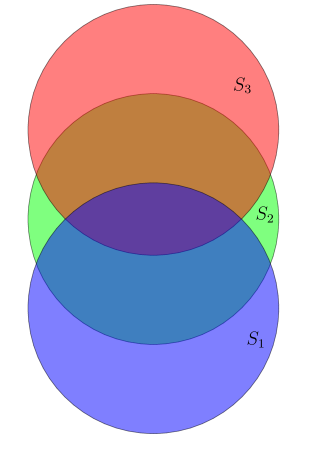
(a) Simplest Degenerate Case: $S_{1}\cap S_{3}\subset S_{2}$

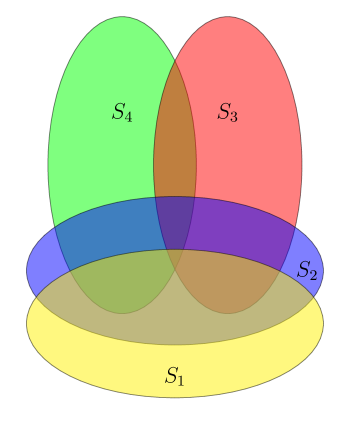
(b) More Complicated Example: $S_{3}\cap S_{4}\cap S_{1}\subset S_{2}$

Figure 1: Simple cases of degeneracy

To be clear, we shall always assume coverage and irredundancy, assumption of genericity is always stated explicitly. Having defined the basic structures, we reiterate the problem: given a sensor configuration ${\mathbf{S}}$ and a sensor measurement vector ${\mathbf{n}}$ our aim is to investigate the problems of finding the range of possible overall values consistent with ${\mathbf{S}}$ and ${\mathbf{n}}$.

II-A Simplicial Complex Formulation

It is possible to provide a description of a sensor configuration in terms of a geometrical object called a simplicial complex. In this context, a simplicial complex is defined to be a collection of subsets $\Sigma$ of the set $\{1,2,\ldots,R\}$, where $R$ is the number of sensors, with the property that if $\sigma\in\Sigma$ and $\tau\subset\sigma$ then $\tau\in\Sigma$. All singletons $\{r\}$ $(r=1,2,\ldots,R)$ are assumed to be in $\Sigma$, as is the empty set $\emptyset$. The dimension of a simplex $\sigma\in\Sigma$ is just $\#\sigma-1$, where $\#A$ is the number of elements of the set $A$. It is useful to think of points of $\{1,2,\ldots,R\}$ (that is singletons) as vertices, simplices $\sigma$ of dimension $1$ as edges joining the elements of the set $\sigma$, simplices $\sigma$ of dimension $2$ as triangles with vertices the elements of $\sigma$, and so on. The resulting geometrical object is called a geometrical realization of the simplicial complex.

The dimension of a simplicial complex is the maximum of the dimensions of all of its simplices. The subsets of a simplex $\sigma$ of dimension $\dim\sigma-1$ are called the faces of $\sigma$.

This abstract simplicial complex always has a geometrical representation. The Geometric Realization Theorem [17] states that a simplicial complex of dimension $d$ has a geometric representation in ${\mathbf{R}}^{2d+1}$, where abstract simplices are represented by geometrical ones and where the abstract concept of face corresponds to the geometrical faces of a simplex. The geometrical picture is a very useful device in visualising the structure of the problem we have described in Section II, and solutions to some special cases.

A given sensor configuration ${\mathbf{S}}=\{S_{1},S_{2},\ldots,S_{R}\}$ then maps to a simplicial complex, called the nerve of the configuration as follows. The nerve of ${\mathbf{S}}$ is the simplicial complex $\Sigma({\mathbf{S}})$ whose vertices are the numbers $\{1,2,\ldots,R\}$ and where $\sigma\in\Sigma$ if $\bigcap_{r\in\sigma}S_{r}\neq\emptyset$. It is straightforward to check that this is indeed a simplicial complex. This definition is well-known; see for example [17].

The ability of the simplicial complex to represent the intersection structure faithfully breaks down when the sensor configuration is degenerate, as in Fig. 1. In the case of Fig. 1(a), the nerve would consist of all subsimplices of a triangle, but as can be seen there is no distinguished region determined by intersections and differences of sensor regions that represents one of the $1$-simplices. In effect $S_{1}\cap S_{2}\cap S_{3}=S_{1}\cap S_{2}$ so that in the simplicial complex picture two different simplices correspond to the same atom.

This simple example is characteristic, as the following simple theorem shows.

Theorem II.3.

Given a sensor configuration ${\mathbf{S}}$, the correspondence which assigns an atom $\langle i_{1},i_{2},\ldots,i_{t}\rangle$ to the simplex $\sigma=\{i_{1},\ldots,i_{t}\}$ is $1-1$ from the atoms ${\mathfrak{A}}({\mathbf{S}})$ of ${\mathbf{S}}$ to (the simplices of) $\Sigma({\mathbf{S}})$ if and only if the sensor configuration is generic.

Proof.

The assignment of

1. a non-empty atom given by $S_{i_{1}}\cap\ldots\cap S_{i_{t}}$ to the simplex $\sigma=\{i_{1},\ldots,i_{t}\}$ and

2. the empty intersection to $\emptyset$

is a bijection of sets as long as the intersections $S_{i_{1}}\cap\ldots\cap S_{i_{t}}$ are non-empty and distinct with the single exception of the empty set. This is exactly the definition of generic. ∎

III Calculation of the Range of Overall Values

We suppose a sensor configuration ${\mathbf{S}}=\{S_{1},S_{2},\ldots,S_{R}\}$ and sensor measurements $n_{1},n_{2},\ldots,n_{R}$. For each atom $\sigma=\langle i_{1},i_{2},\ldots,i_{r}\rangle$, assume that the amount in that intersection is $m_{\sigma}$. The aim is to calculate all possible overall amounts in the entire region, consistent with the reports from each sensor region. Since atoms are disjoint, this is $\sum_{\sigma\text{ atom}}m_{\sigma}$. An upper bound is the sum of the sensor measurements $\sum_{r=1}^{R}n_{r}$. It is essentially trivial to see that, if the collection of sensor regions is irredundant, this upper bound is indeed the maximum possible. It is achieved by putting all of the value in a sensor region $S_{r}$ into $S_{r}\backslash\bigcup_{r^{\prime}\neq r}S_{r^{\prime}}$.

Before going any further, we formulate the linear programming version of the problem. At this point, the formulation does not require the generic hypothesis, though this will be important later. The variables in the primal linear programming problem are the values in each atom. The constraints in this case are that the values in the atoms that are subsets of any given sensor region have to sum to the sensor measurement for that sensor region, since any such region is a disjoint union of its atoms. The problem is then to minimize the sum of all of the atom values $m_{\sigma}$. Formally, the constraints are

$$\sum_{\stackrel{{\scriptstyle a\subset S_{r}}}{{a\text{ is an atom}}}}m_{a}=n_{r}\ (r=1,2,\ldots,R)$$ (3)

and of course that $m_{a}\geq 0$ for all atoms $a$. To calculate the minimum atom sum consistent with the sensor measurements, it is necessary to find the minimum value of $\sum_{a\text{ atom}}m_{a}$ subject to the constraints in (3). More succinctly, we let $A=A_{{\mathcal{S}}}$, with the subscript dropped if the meaning is clear, be the matrix corresponding to the linear equations given in (3); that is the $\sigma,r$ entry of $A_{{\mathcal{S}}}$ is $1$ if the atom $\sigma$ is in the sensor region $S_{r}$ and $0$ otherwise. The sensor measurement vector is ${\mathbf{n}}=(n_{1},n_{2},\ldots,n_{R})$ and the atom value vector is $\mathbf{m}=(m_{a})$. Then the linear programming formulation gives that the minimal value for this sensor configuration ${\mathbf{S}}$ and sensor measurement vector ${\mathbf{n}}$ is

$$\mathfrak{m}({\mathbf{S}},{\mathbf{n}})=\min\{{\mathbf{1}}\cdot\mathbf{m}:A\mathbf{m}={\mathbf{n}},\quad\mathbf{m}\geq 0\},$$ (4)

where $\cdot$ indicates the dot product of the two vectors, so that ${\mathbf{1}}.\mathbf{m}$ is the sum of the entries in $\mathbf{m}$.

The following theorem then addresses the range of values.

Theorem III.1.

Given a sensor configuration ${\mathbf{S}}=(S_{1},S_{2},\ldots,S_{R})$ and sensor measurements ${\mathbf{n}}=(n_{1},n_{2},\ldots,n_{R})$, every (real) value between the maximum and minimum overall value is achievable.

Proof.

The function

$$f(\mathbf{m})=\sum_{a\text{ atom}}m_{a}$$

is continous as well as defined on a bounded, convex polytope which is compact, and connected. This function $f(\mathbf{m})$ then satisfies the intermediate value theorem. ∎

The integer case is more difficult (and interesting). We have the following theorem.

Theorem III.2.

If ${\mathbf{S}}$ is generic, then for every set of sensor managements that are integers, every integer value between the minimum overall (integer) count and maximum overall count is achievable by integer assignments to atoms.

Proof.

It is enough to observe that if ${\mathbf{n}}$ is the sensor measurement vector and $k$ is a possible achievable integer value for the overall count, then so is $k+1$ unless $k$ is the maximum possible count. Suppose first that there is no target in an intersection $S_{i}\cap S_{j}$ with $i\neq j$. Then $k$ is the maximum possible count. Otherwise, suppose that a target $t$ is in $S_{i}\cap S_{j_{1}}\cap\cdots\cap S_{j_{r}}$, and in no other sensor regions.

This target is moved into $\bigl{(}S_{j_{1}}\cap S_{j_{2}}\cap\cdots\cap S_{j_{r}}\bigr{)}\backslash S_{i}$, which is possible because of genericity. Then insert another target in $S_{i}\backslash\bigcup_{i=1}^{r}S_{j_{i}}$. This keeps the sensor measurement for every sensor region unchanged but increases the overall value by $1$. Moreover, it is clear that integers are assigned to atoms by this proof. ∎

We note that the genericity condition is required here, though a somewhat weaker one would suffice. The first configuration in Figure 1 fails to be generic but still has the property that the range of integer overall values forms an interval for any sensor measurement vector. On the other hand, consider the sensor configuration in Figure 2.

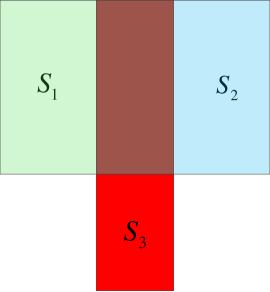
Figure 2: Example where the integer values do not form an interval.

If each sensor region has a count of $1$, then $3$ is clearly the maximum count and $1$ is the minimum, but there is no achievable overall count of $2$ with integer sensor measurements.

It is clear that the maximum overall count associated with integer measurements is the same as the maximum real value associated with those measurements since this is just the sum of the individual sensor counts. On the other hand, this is clearly not the case for the minimum overall value. To see this, consider the case of three sensor regions $S_{1},S_{2},S_{3}$ with only pairwise non-empty intersections: $S_{i}\cap S_{j}\neq\emptyset$ for all $i,j=1,2,3$. In this case, as we shall see later, the minimum overall value is $\frac{n_{1}+n_{2}+n_{3}}{2}$ where $n_{i}$ is the count in region $S_{i}$. As this is not always an integer it cannot be achieved by integer atom values. One might ask whether the smallest integer greater than or equal to this minimum value is achievable by integer atom counts. We have been unable to definitively answer this question, though our experiments suggest that it is always true for generic sensor configurations.

In principle (4) provides a mechanism for calculation of the minimum, and therefore by Theorem III.1 the entire range of possible values, but for large numbers of sensors it becomes impractical. Moreover it suffers the problem that, whenever the sensor value changes, an entirely new calculation is needed. What is required is a formulation of the problem that provides a simple machine to go from sensor measuremens to minimal overall value. This machine should itself be only dependent on the geometry of the sensor regions, with only the inputs of sensor measurements changing. In other words, we would prefer a computable formula into which insertion of the sensor measurements presents the value of (4).

Progress towards such a solution, is obtained via the dual linear programming problem. Since the formulation in (4) is in standard form, the dual problem is (see [18], p.128) expressed in terms of dual variables ${\mathbf{y}}=(y_{r})$ indexed by sensor regions and states

$$\max\{{\mathbf{n}}\cdot{\mathbf{y}}:A^{T}{\mathbf{y}}\leq{\mathbf{1}}\}.$$ (5)

The key difference between this and the usual dual-primal formulation (see [18]) is that, because the primal is stated in terms of equalities, the dual variables have no restrictions other than the linear inequality $A^{T}{\mathbf{y}}\leq{\mathbf{1}}$; in particular, ${\mathbf{y}}$ is not required to be non-negative. As a result the feasible region (the convex set described by the constraints) is not, in general, compact. Existence of solutions therefore becomes an issue.

As an illustration of the problems that can arise consider the case given in Fig. 1(a). The matrix $A$ is obtained as

$$A=\begin{pmatrix}1&0&0&1&0&1\\ 0&1&0&0&1&1\\ 0&0&1&1&1&1\\ \end{pmatrix},$$ (6)

and the dual constraint becomes

$$A^{T}{\mathbf{y}}\leq 1.$$ (7)

This has a solution $(1,1,-1)$ which gives the maximum for $n_{1}=1,n_{2}=1,n_{3}=1$ (and indeed for any values for which $n_{3}\leq\min(n_{1},n_{2})$). It is easy to see that this is an extreme point of the convex (non-compact) polytope specified by (7).

Generally, having to deal with a dual polytope that is not non-negative causes problems and leads to complications in calculating the minimum value. However, many of the potential issues disappear because of the specific nature of the problem. The feasible region is always non-empty: $(\frac{1}{R},\frac{1}{R},\frac{1}{R},\ldots,\frac{1}{R})$ is always in it for example, and the region is bounded above: $y_{r}\leq 1$ for all $r$. It follows by [18] that there is a solution of the dual problem and it equals the solution of the primal. It follows too that the minimum value is exactly the solution of the dual problem, and that once the extreme points of the dual polytope are found it is a simple matter to take their inner products with the sensor measurement vector ${\mathbf{n}}$ and find its maximum to calculate the minimum count. This means that the polytope, or rather its set of extreme points, provides the computational machine needed. We call this polytope the fusion polytope for the given sensor configuration and denote it by ${\mathcal{C}}({\mathbf{S}})$. It is, obviously, only dependent on the sensor configuration. We state this key result as a theorem.

Theorem III.3.

Given a sensor configuration ${\mathbf{S}}$, with fusion polytope ${\mathcal{C}}({\mathbf{S}})$, for any sensor measurement vector ${\mathbf{n}}$,

$$\mathfrak{m}({\mathbf{S}},{\mathbf{n}})=\max\{{\mathbf{n}}\cdot{\mathbf{e}}:{\mathbf{e}}\text{ is an extreme point of ${\mathcal{C}}({\mathbf{S}})$}\}.$$ (8)

Naturally, in the case of a counting, rather than a continuum problem, the solution needs to be an integer, but the smallest integer greater than the actual minimal real solution provides the minimum in that case. We reiterate that, by passage to the dual linear programming problem, the methods to calculate minimum sensor measurements is reduced to testing certain “universal” vertices against the sensor readings. Once the extreme points of the fusion polytope are identified, a formula for the minimum that involves sensor readings as variables is immediate. Indeed there are some extreme points that are unnecessary for this calculation: for instance if ${\mathbf{e}}$ and ${\mathbf{e}}^{\prime}$ are extreme points and $e_{i}^{\prime}\geq e_{i}$ for all $i$ then there is no need to include ${\mathbf{e}}$ in the maximization in (8). We say that ${\mathbf{E}}$ is a dominant extreme point if there is no such ${\mathbf{e}}^{\prime}$. Evidently it is only necessary to list all dominant extreme points for the purposes of (8).

Despite the existence of solutions to the dual problem, the calculation of (dominant) extreme points of the fusion polytope appears hard in general, and we currently have no solution that applies across most situations. Even in some simple cases resulting from graphical models, studied by [19], where the polytope is given by $x_{i}\geq 0$ and $\Sigma_{i\in Q}x_{i}\leq 1$ over cliques $Q$, maximization of a linear objective function over $\operatorname{QSTAB}(G)$ (see Section IV for the definition) is known to be NP-complete.

It turns out, somewhat surprisingly, that the issue of the fusion polytope not residing in the positive orthant is exactly that of non-genericity.

Theorem III.4.

Let the sensor configuration ${\mathbf{S}}$ be generic, and let ${\mathcal{C}}({\mathbf{S}})$ denote the fusion polytope specified by (5). Then

$$\max_{\mathbf{c}\in\mathcal{C}(\mathbf{S})}\mathbf{n}\cdot\mathbf{c}=\max_{\mathbf{c}\in\mathcal{C}(\mathbf{S})\cap P}\mathbf{n}\cdot\mathbf{c}$$ (9)

where $P$ is the positive orthant: $P=\{{\mathbf{y}}:y_{r}\geq 0\ \text{for all $r$}\}$. The converse of this statement is true. If (9) is true then the sensor configuration is generic.

Proof.

Fix ${\mathbf{n}}$ and suppose that $\widetilde{{\mathbf{y}}}$ is an extreme point of $\mathcal{C}(\mathbf{S})$ for which

$${\mathbf{n}}\cdot\widetilde{{\mathbf{y}}}=\max_{{\mathbf{c}}\in\mathcal{C}(\mathbf{S})}{\mathbf{n}}\cdot{\mathbf{c}},$$ (10)

and assume that $\widetilde{{\mathbf{y}}}\not\in P$. Suppose further that there is no extreme point of $\mathcal{C}(\mathbf{S})$ that is non-negative, at which the maximum is achieved. We may assume, without loss of generality that the first $s$ coordinates $\widetilde{{\mathbf{y}}}_{1},\widetilde{{\mathbf{y}}}_{2},\ldots,\widetilde{{\mathbf{y}}}_{s}$ of $\widetilde{{\mathbf{y}}}$ are all negative and that all subsequent coordinates of $\widetilde{{\mathbf{y}}}$ are non-negative. Let $\widetilde{{\mathbf{y}}}^{\prime}$ be the vector $\widetilde{{\mathbf{y}}}$ with the first $s$ coordinates replaced by $0$.

Let $A$ be the defining matrix for the linear programming problem as in (4). The generic property entails that if ${\mathbf{a}}$ is a row of $A^{T}$ then a row vector ${\mathbf{a}}^{\prime}$ for which the coordinatewise product satisfies ${\mathbf{a}}\cdot{\mathbf{a}}^{\prime}={\mathbf{a}}^{\prime}$ is also a row of $A^{T}$. It follows that, for any row ${\mathbf{a}}$ of $A^{T}$, there is a row of $A^{T}$ which has the first $s$ rows of ${\mathbf{a}}$ replaced by $0$. As a result, ${\mathbf{a}}\cdot\widetilde{{\mathbf{y}}}^{\prime}\leq 1$ for all rows ${\mathbf{a}}$ of $A$. Thus $\widetilde{{\mathbf{y}}}^{\prime}\in\mathcal{C}(\mathbf{S})\cap P$. Moreover, clearly

$${\mathbf{n}}\cdot\widetilde{{\mathbf{y}}}^{\prime}\geq{\mathbf{n}}\cdot\widetilde{{\mathbf{y}}}.$$ (11)

The conclusion follows.

For the converse, we observe that the constraints in the dual problem are labelled and determined by atoms. In consequence ${\mathcal{C}}({\mathbf{S}}_{\text{gen}})$ is a subset of ${\mathcal{C}}(S)$. However, in the case of ${\mathcal{C}}(S)\cap P$, only the constraints that correspond to the highest dimensional simplices (or equivalently the largest number of sensor regions in the intersection forming the atom) are relevant, since any constraint imposed in respect of such a simplex is stronger than one corresponding to a simplex contained in it. The highest dimensional constraints are common to both ${\mathbf{S}}$ and to ${\mathbf{S}}_{\text{gen}}$, so that

$${\mathcal{C}}({\mathbf{S}})\cap P={\mathcal{C}}({\mathbf{S}}_{\text{gen}})\cap P.$$ (12)

Now, for a sensor measurement vector ${\mathbf{n}}$,

$$\max\{{\mathbf{y}}\cdot{\mathbf{n}}:{\mathbf{y}}\in{\mathcal{C}}({\mathbf{S}})\} \geq\max\{{\mathbf{y}}\cdot{\mathbf{n}}:{\mathbf{y}}\in{\mathcal{C}}({\mathbf{S}})\cap P\}$$ (13)

$$=\max\{{\mathbf{y}}\cdot{\mathbf{n}}:{\mathbf{y}}\in{\mathcal{C}}({\mathbf{S}}_{\text{gen}})\cap P\}$$

$$=\max\{{\mathbf{y}}\cdot{\mathbf{n}}:{\mathbf{y}}\in{\mathcal{C}}({\mathbf{S}}_{\text{gen}})\}.$$

Thus if

$$\max\{{\mathbf{y}}\cdot{\mathbf{n}}:{\mathbf{y}}\in{\mathcal{C}}({\mathbf{S}})\}=\max\{{\mathbf{y}}\cdot{\mathbf{n}}:{\mathbf{y}}\in{\mathcal{C}}({\mathbf{S}})\cap P\},$$ (14)

then

$$\max\{{\mathbf{y}}\cdot{\mathbf{n}}:{\mathbf{y}}\in{\mathcal{C}}({\mathbf{S}})\}=\max\{{\mathbf{y}}\cdot{\mathbf{n}}:{\mathbf{y}}\in{\mathcal{C}}({\mathbf{S}}_{\text{gen}})\}.$$ (15)

If ${\mathbf{S}}$ is not generic, then there is some intersection $S_{i_{1}}\cap S_{i_{2}}\cap\cdots\cap S_{i_{R}}$ contained in a union of some different sensor regions $S_{j_{1}},S_{j_{2}},\ldots,S_{j_{T}}$. Consider a sensor measurement vector which assigns $1$ to each of the sensor regions $S_{i_{r}}$ $(r=1,2,\ldots,R)$, and $0$ to every other sensor region.

The minimal overall value for ${\mathbf{S}}$ is at least $2$ because there can be no targets in the intersection $S_{i_{1}}\cap S_{i_{2}}\cap\cdots\cap S_{i_{R}}$. On the other hand for the corresponding sensor measurement in the generic case the minimal overall value is $1$, since there can be just one target in the intersection $S_{i_{1}}\cap S_{i_{2}}\cap\cdots\cap S_{i_{R}}$. ∎

This result considerably simplifies calculations in the generic case. We call $\mathcal{C}(\mathbf{S})\cap P$ the positive fusion polytope, though the word “positive” will be dropped where there is no likelihood of confusion. One simple consequence of this result is that in the generic case, if the sensor measurement increases; that is, if we have two sensor measurement vectors ${\mathbf{n}}=(n_{1},n_{2},\ldots,n_{R})$ and ${\mathbf{n}}^{\prime}=(n^{\prime}_{1},n^{\prime}_{2},\ldots,n^{\prime}_{R})$ where $n_{i}\geq n_{i}^{\prime}$, then the minimum increases, or at least does not decrease. This may seem, at first sight obvious, but it is quickly apparent from Theorem III.4 that it is not true in the degenerate case, and indeed this is a defining characteristic of genericity. As simple example consider the case of Figure 1(b). If the sensor measurement vector is $(1,0,1)$, then the minimum overall value is $2$, whereas if the sensor measurement vector is $(1,1,1)$ the minimum overall value is $1$.

In the generic case, the linear programming problem is expressible entirely in terms of the simplicial complex. The translation is as follows. For each vertex of the simplicial complex (sensor region) we have the following constraint:

$$\sum_{\sigma\text{ contains vertex $v$}}m_{\sigma}=n_{v},$$ (16)

corresponding to the constraint (3) in the “region” formulation. In addition, of course $m_{\sigma}\geq 0$. We need to minimize

$$\sum_{\sigma}m_{\sigma},$$ (17)

subject to these constraints. The dualization results in the following problem expressed in terms of the geometry of the simplicial complex.

$$\max\{\sum_{r}y_{r}:\sum_{r\in\sigma}y_{r}\leq 1,\ (\sigma\in\Sigma),\ y_{r}\geq 0\ (r=1,2,\ldots,R)\}.$$ (18)

The fusion polytope is then, with some abuse of notation,

$${\mathcal{C}}(\Sigma)=\{{\mathbf{y}}=(y_{r}):\sum_{r\in\sigma}y_{r}\leq 1,\ (\sigma\in\Sigma),\ y_{r}\geq 0\ (r=1,2,\ldots,R)\}.$$ (19)

Observe that if $\sigma\subset\sigma^{\prime}$ are simplices then $\sum_{r\in\sigma}y_{r}\leq\sum_{r\in\sigma^{\prime}}y_{r}$ so that the only inequalities that need be considered in defining ${\mathcal{C}}(\Sigma)$ are those that are maximal; that is, are not contained in any larger simplex. Thus in the case of three regions with all possible intersections, so that the simplicial complex is the triangle and all of its subsimplices, the only inequality (other than non-negativity) that is needed is $y_{1}+y_{2}+y_{3}\leq 1$. It follows immediately that the extreme points of $\Sigma$ in this case are $(1,0,0),\ (0,1,0),\ (0,0,1)$ and the minimal count is $\max(n_{1},n_{2},n_{3})$.

As another example consider the case where the simplicial complex $\Sigma$ consists of the faces of a tetrahedron. This corresponds to four regions such that each triple intersection is non-empty but the quadruple intersection is empty. The constraint matrix for the dual problem (corresponding only to highest dimensional simplices) is

$$A^{T}=\begin{pmatrix}1&1&1&0\\ 1&1&0&1\\ 1&0&1&1\\ 0&1&1&1\\ \end{pmatrix}.$$ (20)

It is fairly easy to see that the fusion polytope in this case has extreme points $(1,0,0,0)$, $(0,1,0,0)$, $(0,0,1,0)$, $(0,0,0,1)$ and $(\frac{1}{3},\frac{1}{3},\frac{1}{3},\frac{1}{3})$, and so the minimum count is

$$\max(n_{1},n_{2},n_{3},n_{4},\frac{1}{3}(n_{1}+n_{2}+n_{3}+n_{4})).$$ (21)

IV Graphs

There are a number of cases where the minimum estimation problem can be posed in terms of constructs on graphs. This happens in various ways. Even when such a reformulation is possible, it does not always provide a feasible approach to computation of the minimum; rather these formulations and the effort in the graph theory community to solve the corresponding problems suggest that the minimum estimation problem is difficult.

IV-A The Fractional Stable Set

To describe the ideas, we consider a graph ${\mathcal{G}}=({\mathcal{V}},{\mathcal{E}})$. A set of vertices $U\subset{\mathcal{V}}$ is called a stable set if no two distinct elements of $U$ have an edge joining them; that is, if $u_{1}\neq u_{2}$, $u_{1},u_{2}\in U$, then $(u_{1},u_{2})\not\in{\mathcal{E}}$. The convex hull

$$\operatorname{STAB}(G)=\operatorname{co}\{{\mathbf{1}}_{U}:U\text{ is a stable set of vertices}\}.$$ (22)

is called the stable set polytope. The fractional stable set polytope of a graph is

$$\operatorname{FRAC}(G)=\{(x_{v})_{v\in{\mathcal{V}}}:x_{v}\geq 0,\ x_{v_{1}}+x_{v_{2}}\leq 1,\ (v,v_{1},v_{2}\in{\mathcal{V}}),\ (v_{1},v_{2})\in{\mathcal{E}}\}.$$ (23)

It is straightforward, and well known that $\operatorname{STAB}(G)\subset\operatorname{FRAC}(G)$, and that the latter is exactly the fusion polytope for the situation where the $R$ sensor regions correspond to the vertices of the graph, pairwise intersections correspond to edges, and there are no triple or higher intersections; that is, where the nerve is just a graph. In this context some results exist; a good reference is the notes of Wagler [20], but even this relatively simple case appears to produce no simple algorithm for computation of the extreme points. Here is an important theorem.

Theorem IV.1 (Grötschel, Lovász, Schrijver, [21]).

  

1. $\operatorname{STAB}(G)=\operatorname{FRAC}(G)$ if and only if $G$ is bipartite with no isolated vertices;

2. The extreme points of $\operatorname{STAB}(G)$, regarded as functions on the vertices of $G$, all have values $0$ and $1$;

3. The extreme points of $\operatorname{FRAC}(G)$ all have values $0$, $1/2$, $1$.

We illustrate these ideas with the following simple example.

Example IV.2.

We consider the case when the regions $S_{1},S_{2},\ldots,S_{R}$ satisfy $S_{i}\cap S_{i+1}\neq\emptyset$, $S_{1}\cap S_{R}\neq\emptyset$ and these are the only non-empty intersections. The nerve is a graph with $R$ vertices connected in a cycle. A collection of extreme points involve just $0$s and $1$s which satisfy the following rules:

1. every $1$ is isolated, that is, $11$ does not appear;

2. no sequences with three adjacent $0$s appear.

Thus, between every pair of $1$s either a single $0$ or a pair of $0$s appears. If $R$ is even, all extreme points are of this form, but if $R$ is odd there is an additional extreme point of the form ${\mathbf{d}}=(\frac{1}{2},\frac{1}{2},\ldots,\frac{1}{2})$. When $R$ is even ${\mathbf{d}}$ is a convex combination of two $0$-$1$ extreme points and so is not extreme.

While the preceding discussion shows how graph theoretic ideas apply for the case where there are no non-trivial triple intersections, there are some other situations where graph theory is applicable. A construct on graphs related to the stable and the fractional stable set polytopes is obtained as follows. We recall that a clique in the graph $G$ is a set $Q$ of vertices that as the induced subgraph of $G$ is complete; that is, each pair of vertices in $Q$ is connected by an edge. Now we define

$$\operatorname{QSTAB}(G)=\{(x_{v})_{v\in{\mathcal{V}}}:x_{v}\geq 0,\ \sum_{v\in Q}x_{v}\leq 1,\ \text{$Q$ is a clique in $G$}\}$$ (24)

The $\operatorname{QSTAB}$ construction permits representation of the fusion polytope for other sensor configurations than just those with only pairwise intersections. For instance, consider Figure 3. In this case, the $2$-simplices are present and so the nerve is not a graph. However, the cliques of the $1$-skeleton $G$ are just the two $2$-simplices and so $\operatorname{QSTAB}(G)$ is the fusion polytope. On the other hand if the sensor regions are as in Figure 4 then the simplicial complex is $1$-dimensional and comprises the edges of a triangle. In this case the single clique consists of all vertices of the graph and so $\operatorname{QSTAB}$ is not the same as the fusion polytope.

A flag complex is an abstract simplicial complex in which every minimal nonface has exactly two elements [22]. In essence, any flag complex is the clique complex (that is, the set of all cliques) of its $1$-skeleton. For example, if three edges of a $2$-simplex are in the simplicial complex in question, then so is the $2$-simplex itself. More generally, if all of the faces of a simplex are in the simplicial complex, then so is the entire simplex. The boundary of a $2$-simplex does not form a flag complex, but the $2$-simplex itself does. We have the following theorem.

Theorem IV.3.

Given sensor regions $S_{1},S_{2},\ldots,S_{R}$ which form a generic sensor configuration, the fusion polytope is identified with $\operatorname{QSTAB}(G)$ via the inclusion of a graph $G$ as the $1$-skeleton of the simplicial complex of the sensor configuration if and only if it is a flag complex.

Proof.

We assume throughout that the sensor configuration is generic. Next, assume that the simplicial complex of the sensor configuration is a flag complex $K$. Then $K$ is the clique complex of its $1$-skeleton $G$ by definition. $\operatorname{QSTAB}(G)$ is determined by all of the cliques and the fusion polytope is determined by the simplicial complex. Since this is a clique complex by definition, the fusion polytope is identified with $\operatorname{QSTAB}(G)$.

For the reverse direction, assume that the fusion polytope is identified with $\operatorname{QSTAB}(G)$, and that $G$ is the $1$-skeleton of the simplicial complex of the sensor configuration. Since the fusion polytope is determined by this simplicial complex, and $\operatorname{QSTAB}(G)$ is determined by all cliques, there is a correspondence between simplicies and cliques, which means any simplex of the simplicial complex is a clique of $G$. The simplicial complex is then a flag complex by definition. ∎

Much work has been done on $\operatorname{QSTAB}(G)$ by many authors; see, for instance, [23] for several references. Since we are interested in the extreme points of $\operatorname{QSTAB}(G)$ in situations when $\operatorname{QSTAB}(G)$ is the fusion polytope of a sensor configuration, the following result is important. It will require the definition of a perfect graph. First we need to know that a subgraph of $G$ is induced if is obtained by taking a subset of the vertices of $G$ and all edges from $G$ with endpoints in the subset. A graph $G$ is perfect if, for every subgraph $H$ of $G$, the chromatic number of $H$ is equal to the size of the largest clique of $H$. All bipartite graphs are perfect, whereas an odd cycle is not.

Theorem IV.4 ([24]).

Let $G$ be a graph. Then $\operatorname{STAB}(G)=\operatorname{QSTAB}(G)$ if and only if $G$ is perfect.

Of course, if $\operatorname{STAB}(G)=\operatorname{QSTAB}(G)$ then the dominant extreme points must all take the values $0$ and $1$ and are fairly easy to write down; indeed they are the characteristic functions of maximal stable sets.

Figure 3: Example where $QSTAB(G)$ is the Fusion Polytope

Figure 4: Example where $QSTAB(G)$ is different from the Fusion Polytope

V The Two Dimensional Case

V-A Quadruple Intersections

At this point we consider planar sensor regions of various kinds. As an example, consider an “inflated tiling” of the plane; that is, a standard regular tiling by rectangles, illustrated in Figure 5, where the tiles are slightly inflated to create overlapping regions.

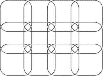
Figure 5: Tiling by Rectangles

To be precise, the unit square $[0,1]\times[0,1]$ in the plane is covered by $Q^{2}$ regions as in the figure. Note that there are quadruple intersections but no higher, so that the nerve will be $3$-dimensional. The regions are labelled $(S_{ij})_{i,j=1}^{Q}$ in matrix style, and the following quadruple intersections, and only these are non-empty:

$$S_{ij}\cap S_{(i+1)j}\cap S_{i(j+1)}\cap S_{(i+1)(j+1)}.$$ (25)

In addition double and triple intersections forced by these quadruple ones are present. One might expect that this kind of sensor configuration would be relatively easily to handle. Unfortunately it fails to be generic, specifically there are relations such as:

$$S_{11}\cap S_{22}\subset S_{12}\cup S_{21},$$ (26)

so that the potential atom $S_{11}\cap S_{22}\cap S_{12}^{c}\cap S_{21}^{c}\cap\bigcap_{i>2\text{ or }j>2}S_{ij}^{c}$ is empty. It follows, by Theorem III.4, that the fusion polytope is not in the positive orthant. Indeed the point $(-1,1,1,-1)$ is an extreme point of the fusion polytope for the case of just four regions $S_{11},S_{12},S_{21},S_{22}$.

It turns out that this situation is typical. Indeed, any configuration of four regions in the plane that satisfies some fairly reasonable topological assumptions and that has a quadruple intersection fails to be generic, as the following theorem shows. In order to describe the result, more precision will be needed about the nature of regions and their intersections than has been required so far. At this point we shall introduce the topological constraints predicted when atoms were first defined in II.1. We need to make some minor adjustments to definitions in order to enable us to use topological arguments.

For this purpose, a regular sensor region $S$ is a bounded open set in the plane of which the boundary $\partial S$ is a simple piecewise smooth closed curve. A regular sensor configuration is one comprising regular sensor regions. We need also to redefine the notion of an atom. In this case, we replace each set of the form $S_{i}^{c}$ in (16) by its interior $\overline{S_{i}}^{c}$, but we still demand that an atom is non-empty, though we will use the phrase that the “atom is represented” to mean exactly that. Note that atoms are always open with this definition. A regular sensor configuration is said to be generic if an intersection of sensor regions is not contained in a union of different sensor regions.

A regular sensor configuration $\{S_{1},S_{2},S_{3},\ldots,S_{R}\}$ with $X=\cup_{r=1}^{R}S_{r}$ is said to be normal if the boundaries of any two sensor regions intersect in at most two points, and there are no points of triple intersection of boundaries of sensor regions. We also require that boundaries of atoms are simple closed curves; these are, of course made up of segments of boundaries of sensor regions. Observe that, by the Jordan-Schoenflies Theorem [25], these conditions imply that both closures of sensor regions and closures of atoms are homeomorphic to closed discs. For the rest of this section we assume that all sensor regions are regular and just refer to them as sensor regions.

Theorem V.1.

For a normal sensor configuration $\mathbb{S}=\{S_{1},S_{2},S_{3},S_{4}\}$ with closure a simply-connected closed set in the plane $\mathbb{R}^{2}$, at least two atoms are not represented; that is, are empty. The sensor configuration is not generic.

Proof.

A simplicial complex is constructed with the intersection points of boundaries of sensor regions as vertices, the segments of the boundaries between the intersection points as edges and the atoms of the sensor configuration as faces. This is a planar simplicial complex. By our assumption on intersections of boundaries of sensor regions, there are at most $12$ vertices ($6+4+2$) and the degree of each vertex is $4$ in the graph which is the $2$-skeleton of the simplicial complex. Furthermore, the number of edges is twice of the number of vertices, by the condition on the boundaries of atoms. Since the Euler characteristic of the closure of the union of the sensor regions, is $1$, $v-e+f=1$, we have $v=f-1$. Since $v\leq 12$, $f\leq 13$ is obtained; that is, there are at least two atoms not represented. ∎

If the condition of normality is relaxed to allow the boundary of one sensor region to intersect the boundary of another in $4$ points, then there will be two more vertices in the corresponding graph and the number of possible faces will be equal to $15$. All atoms can then be represented and connected, as the example in Figure 6 demonstrates. Furthermore, if more pairwise intersections of boundaries of sensor regions with $4$ points appear, all atoms still can still be represented, however, will be disconnected as shown in Figure 7.

Figure 6: Four Regions in the Plane with All Atoms Represented and Connected

Figure 7: Four Regions in the Plane with All Atoms Represented

Despite this failure of genericity for the inflated rectangular tilings it is still possible to use the dual linear programming technique in this case. As already noted, the fusion polytope is no longer in the positive orthant and the simplifications associated with that property are not available. It is still possible, however, to place a lower bound on the polytope as the following result indicates, and the region need not be rectangular for this to happen. The following notation will be useful:

$$D_{\epsilon}=\{{\mathbf{x}}\in{\mathbf{R}}^{2}:\|{\mathbf{x}}-I^{2}\|<\epsilon\}$$ (27)

and $I^{2}=[0,1]^{2}$ is the unit square. We can use any one of a number of (convex) norms, the key features being that

$$D_{\epsilon}\cap\bigl{(}(0,1)+D_{\epsilon}\bigr{)}\cap\bigl{(}(1,0)+D_{\epsilon}\bigr{)}\cap\bigl{(}(1,1)+D_{e}\bigr{)}\neq\emptyset.$$ (28)

Also $\epsilon$ needs to be small enough to prohibit intersections of the form

$$D_{\epsilon}\cap\bigl{(}(2,0)+D_{\epsilon}\bigr{)}\text{ or }D_{\epsilon}\cap\bigl{(}(0,2)+D_{\epsilon}\bigr{)}.$$

Theorem V.2.

Let $T$ be a region in the plane that is a union of inflated squares based on the integer lattice. Thus

$$T=\bigcup_{r=1}^{R}(m_{r},n_{r})+D_{\epsilon},$$ (29)

and let the sensor regions be $(m_{r},n_{r})+D_{\epsilon}$. Then no point in the corresponding fusion polytope has a coordinate less than $-1$.

Proof.

The constraints of the fusion polytope correspond to non-empty intersections of the sensor regions, and these are of four kinds (only the translating integer pairs are listed):

• Squares: $\sigma=\{(n,m),(n,m+1),(n+1,m),(n+1,m+1)\}$.

• Corners: $\ell=\{(n,m),(n,m+1),(n+1,m)\}$ and all variants of this by rotations through $90^{\circ}$ and reflections.

• Segments:$\gamma=\{(n,m),(n,m+1)\}$ and all rotations through $90^{\circ}$.

• Singletons: $\alpha=\{(n,m)\}$.

Thus, for a square we obtain the constraint,

$$x_{(n,m)}+x_{(n,m+1)}+x_{(n+1,m)}+x_{(n+1,m+1)}\leq 1,$$ (30)

with similar constraints for the corners and segments. Singletons give rise to the constraint $x_{(n,m)}\leq 1$.

Write $A$ for the matrix whose rows are obtained from the constraints. The columns of $A$ are indexed by $r=1,\ldots,R$. The fusion polytope is then $C_{F}=\{{\mathbf{x}}\in{\mathbf{R}}^{2}:A{\mathbf{x}}\leq 1\}$.

The extreme points of $C_{F}$ are all obtained as the unique solutions of equations of the form $A_{1}{\mathbf{x}}={\mathbf{1}}$ where $A_{1}$ is obtained by choosing rows from $A$ that form a basis for ${\mathbf{R}}^{N}$. In addition, of course, ${\mathbf{x}}\in C_{F}$, so $A_{1}^{c}{\mathbf{x}}\leq{\mathbf{1}}$ for the remaining rows $A_{1}^{c}$ of $A$. We write $W(A_{1})$ for the collection of squares, corners, segments and singletons corresponding to the rows of $A_{1}$.

Now suppose that the $(n_{r},m_{r})$th coordinate is less than $-1$ and let $R$ be a region in $W(A_{1})$ containing $(n_{r},m_{r})$. Clearly, $R$ cannot be a singleton. Neither can it be a segment or a corner since the sum over $R$ has to be $1$ and each $x_{(n,m)}\leq 1$. Suppose then that $R$ is a square. This would imply that the sum over the members of the square other than $(n_{r},m_{r})$ is at least $2$. But these form a corner and so the sum has to be less than $1$. This provides a contradiction and proves the result. ∎

Even though $C_{F}$ is not compact we can still use its extreme points to count. The following result follows quickly from standard results on convex polyhedra.

Lemma V.3.

If ${\mathbf{c}}$ is a vector in ${\mathbf{R}}^{N}$ in the positive quadrant then

$$\sup\{{\mathbf{c}}\cdot{\mathbf{x}}:{\mathbf{x}}\in C_{F}\}=\max\{{\mathbf{c}}\cdot{\mathbf{e}}:{\mathbf{e}}\in\operatorname{{Ext}}C_{F}\}$$ (31)

where $\operatorname{{Ext}}C_{F}$ is the set of extreme points.

V-B Hexagons

If instead of using inflated rectangular tilings, we employ inflated hexagonal tilings, the genericity problems disappear. Let $H$ be the regular hexagon centred at the origin in ${\mathbf{R}}^{2}$ and with vertices at $(0,\pm 1)$,$(\pm\frac{1}{2},\pm\frac{\sqrt{3}}{2})$ and consider translates of this via the hexagonal lattice. These tesselate the plane in a honeycomb arrangement. Slight inflations of them have at most $3$-fold intersections and so do not suffer the problems of the rectangular tilings. In this case for a cover of some region in the plane by translates of these inflated hexagons the fusion polytope lies in the positive orthant. Even in this case, though, for large numbers of such inflated hexagons the fusion polytope can become very complicated and its number of extreme points large. We illustrate this with a few examples computed using the polymake package (http://www.polymake.org/doku.php). This is a topic we intend to return to in a later paper.

Consider the tesselation of a region of the plane in Figure 8(a). In fact, of course, we are interested in slight inflations of these hexagons so that the regions overlap. There are obvious triple intersections but no quadruple intersection.

(a) Hexagonal Tesselation of Region in Plane: 30 Hexagons

(b) A $(0,1)$ Extreme Point

Figure 8: Tesselation and Extreme point involving only $0,1$ coefficients

This, incidentally, is almost as large a collection of hexagons as we are reasonably able to handle on a laptop computer in the space of a few days using polymake. According to polymake, the fusion polytope for the collection of 30 hexagons depicted here has nearly 5000 dominant extreme points. Many, in fact most, of these are extreme points involving only $0$ (white), and $1$ (blue) coefficients such as the one in Figure 8(b). The rule for generating such (dominant) extreme points is fairly simple. No two adjacent hexagons can have a coefficient $1$, and the number of $1$s is maximal subject to this constraint.

More interesting are extreme points with coefficients of $1/2$ (yellow) and $0$ (white), such as in Figure 9(a).

(a) Extreme point with $0,\frac{1}{2}$ coefficients

(b) Mixture of $0,1$ and $0,\frac{1}{2}$ extreme point

Figure 9: Extreme points involving $0,\frac{1}{2},1$ coefficients

Here again it would not be too hard to develop a description of the patterns. It is clear that no three hexagons that meet at a point can all have coefficient $1/2$. Moreover, and these appear to be related to the result IV.1 [21]], every example of this kind involves a loop with an odd number of hexagons. There are, however, other possibilities for extreme points. One rather obvious one is a mixture of the preceding two types as is illustrated in Figure 9(b).

More exotic extreme points also arise. To illustrate, consider Figures 10(a) (where grey represents $\frac{1}{4}$ and black $\frac{3}{4}$, and yellow, as before, represents $\frac{1}{2}$), and Figures 10(b) (where green represents $\frac{1}{3}$ and red $\frac{2}{3}$). Coefficients other than $0,1,\frac{1}{2},\frac{1}{3},\frac{2}{3},\frac{1}{4},\frac{3}{4}$ have also been observed. We will discuss these patterns in much more detail in a later paper.

(a) An extreme point with coefficients $0,\frac{1}{2},\frac{1}{4},\frac{3}{4}$

(b) An Extreme Point with coefficients $0,\frac{1}{3},\frac{2}{3}.$

Figure 10: Exotic Extreme Points

VI Bounds and Special Types of Regions

We consider here only (irredundant, covering,) generic sensor configurations. These are entirely represented by their nerves and so are discussed in those terms. Accordingly, we fix a simplicial complex $\Sigma$ which is the nerve of a sensor configuration ${\mathbf{S}}=(S_{1},S_{2},\ldots,S_{R})$. As before, $\mathfrak{m}(\Sigma,{\mathbf{n}})$ denotes the minimum value associated with this configuration and the sensor measurement vector ${\mathbf{n}}$.

The $k$-skeleton of $\Sigma$ is defined to be the subcomplex of $\Sigma$ consisting of those subsets of size $\leq k+1$ (or in other words simplices of dimension $\leq k$ and denoted by $\Sigma^{k}$. We write $\Sigma_{k}$ for the simplicial complex obtained from $\Sigma$ by inserting a new simplex whenever $\Sigma$ contains all of the $k$-faces of that simplex. In other words, if every subset of $\sigma=(i_{1},i_{2},\ldots,i_{r})$ ($1\leq i_{n}\leq R$) of size $k+1$ belongs to $\Sigma$ then $\sigma\in\Sigma$.

The following result is a straightforward observation. Recall that genericity permits us to consider the fusion polytope as a subset of the positive orthant.

Theorem VI.1.

$${\mathcal{C}}(\Sigma_{1})\subset{\mathcal{C}}(\Sigma_{k})\subset{\mathcal{C}}(\Sigma)\subset{\mathcal{C}}(\Sigma^{k})\subset{\mathcal{C}}(\Sigma^{1}),$$ (32)

and so for any measurement vector ${\mathbf{n}}$,

$$\max{\mathbf{n}}=\mathfrak{m}(\Sigma_{1},{\mathbf{n}})\leq\mathfrak{m}(\Sigma_{k},{\mathbf{n}})\leq\mathfrak{m}(\Sigma,{\mathbf{n}})\leq\mathfrak{m}(\Sigma^{k},{\mathbf{n}})\leq\mathfrak{m}(\Sigma^{1},{\mathbf{n}})={\mathbf{1}}.{\mathbf{n}}.$$ (33)

Of course $\Sigma^{2}$ is a graph and so the techniques discussed in Section IV can be applied to the calculation of $\mathfrak{m}(\Sigma^{2},{\mathbf{n}})$.

Some kinds of restrictions on shapes make calculating and bounding the minimal count easier. When the regions are convex subsets of ${\mathbf{R}}^{n}$, Helly’s Theorem is effectively as follows.

Theorem VI.2 ([26]).

If $C_{1},C_{2},\ldots,C_{R}$ are convex subsets of ${\mathbf{R}}^{n}$ with the property that $C_{i_{1}}\cap C_{i_{2}}\cap\cdots\cap C_{i_{n+1}}\neq\emptyset$ for all choices of $i_{k}$, then $C_{1}\cap C_{2}\cap\cdots\cap C_{R}\neq\emptyset$.

In terms of the simplicial complex associated with the sensor regions this yields the following property.

Theorem VI.3.

Let ${\mathbf{S}}=(S_{1},S_{2},\ldots,S_{R})$ be a generic sensor configuration for which the sensor regions are convex subsets of ${\mathbf{R}}^{N}$. Let $\Sigma$ be the corresponding simplicial complex. Then $\Sigma$ contains all of the $N$-dimensional faces of a simplex it must also contain the simplex. In other words $\Sigma_{N}=\Sigma$.

In particular, if the sensor regions are in the plane ${\mathbf{R}}^{2}$ then $\Sigma_{2}=\Sigma$.

Another situation in which it is possible to make further progress concerns a generic collection of sensor regions with the property that every sensor region contains a “uniformly maximal dimensional intersection”; in other words, there is some $M$ such that for every $r$,

$$S_{r}\supset S_{i_{1}}\cap S_{i_{2}}\cap\ldots\cap S_{i_{M+1}}\neq\emptyset,$$

but there are no non-trivial non-empty $M+2$ intersections. This amounts to a “manifold” assumption on the nerve; namely, that every simplex is a subset of one of maximal dimension $M$. In this case, in the dual formulation of the linear programming problem, the only inequalities that need to be considered are the ones involving the maximal dimensional simplices. In this case, ${\mathcal{C}}(\Sigma)={\mathcal{C}}(\Sigma_{M})$, but more importantly, the linear programming problem is significantly simplified because of the reduced number of inequalities. To illustrate this we present the following example.

We describe several generic sensor configurations in terms of the simplicial complex formulation. Let $\sigma_{a}=\{a,b,c,d\}$, $\sigma_{r}=\{r,s,t,u\}$, and $\sigma_{w}=\{w,x,y,z\}$ be three generic tetrahedra given in terms of their vertices in ${\mathbf{R}}^{3}$.

Example VI.4.

1. First consider the sensor configuration comprising $\sigma_{a}$ and $\sigma_{r}$ with $a=r$. In this case all extreme points have coordinates equal to either $0$ or $1$. Only one vertex of each tetrahedron can be assigned a $1$. This is the only restriction, resulting in 10 (dominant) extreme points.

2. Now consider the case where the three tetrahedra are attached in a string: $a=r$ and $u=w$. As the same as the previous case, all extreme points have coordinates equal to either $0$ or $1$.

3. Next, suppose that the three tetrahedra are connected in a cycle: $a=r$ and $u=w$, $x=b$. Then, in addition to the obvious $0,1$ extreme points, there is one $0,\frac{1}{2}$ extreme point with values $\frac{1}{2}$ at $a$, $u$, and $x$.

4. Now suppose that the tetrahedra are connected along edges, say, $(a,b)=(r,s)$ and $(t,u)=(w,x)$. then again all extreme points are $0,1$-valued.

5. Finally consider the case $(a,b)=(r,s)$, $(t,u)=(w,x)$, $(y,z)=(c,d)$. In this case there also $0,\frac{1}{2}$-valued extreme points with supports triangles with one edge in each tetrahedron.

Surprisingly, even if more and more tetrahedra are glued together in such a way, the coordinates of all extreme points still only can be $0$ or $1$, although the number of them increases quickly. We will discuss these conclusions in much more detail in a later paper.

VII Conclusion

This paper introduces methods for obtaining the limits on fusion of simple measurements from multiple sensors. The problem is formulated as one in linear programming and dualized to obtain an object, called the fusion polytope, which is the key device for calculation of the minimum fused value compatible with the data. The fusion polytope is computed in some simple cases. It is shown that when the sensor configuration satisfies a simple property, defined in the paper as genericity, this fusion polytope can be assumed to be in the positive orthant.

It is also shown that under some mild hypotheses genericity is not satisfied when there are four overlapping sensor regions in the plane. Consideration is given to the case of overlapping regions in a hexagonal tiling in the plane. This is a generic situation, but simulations have shown that it still leads to very complex extreme point structures.

We believe that the ideas described here are capable of being extended to more complex situations where data fusion is required.

References

- [1] A. Newell and K. Akkaya, “Self-actuation of camera sensors for redundant data elimination in wireless multimedia sensor networks,” in Proceedings of the 2009 IEEE international conference on Communications, ser. ICC’09. Piscataway, NJ, USA: IEEE Press, 2009, pp. 133–137.
- [2] A. Mittal and L. S. Davis, “Visibility analysis and sensor planning in dynamic environments,” in ECCV (1). Berlin: Springer-Verlag, 2004, pp. 175–189.
- [3] L. Lazos and R. Poovendran, “Stochastic coverage in heterogeneous sensor networks,” ACM Trans. Sen. Netw., vol. 2, pp. 325–358, August 2006.
- [4] Q. Wu, N. S. V. Rao, X. Du, S. S. Iyengar, and V. K. Vaishnavi, “On efficient deployment of sensors on planar grid,” Comput. Commun., vol. 30, pp. 2721–2734, October 2007.
- [5] L. Lazos, R. Poovendran, and J. A. Ritcey, “Probabilistic detection of mobile targets in heterogeneous sensor networks,” in Proceedings of the 6th international conference on Information processing in sensor networks, ser. IPSN ’07. New York, NY, USA: ACM, 2007, pp. 519–528.
- [6] M. L. Connolly, “Computation of molecular volume,” Journal of the American Chemical Society, vol. 107, no. 5, pp. 1118–1124, 1985.
- [7] J. Liang, “Computation of protein geometry and its applications: Packing and function prediction,” in Computational Methods for Protein Structure Prediction and Modeling, ser. Biological and Medical Physics, Biomedical Engineering, Y. Xu, D. Xu, and J. Liang, Eds. New York: Springer New York, 2007, pp. 181–206.
- [8] R. Ghrist and Y. Baryshnikov, “Target enumeration via integration over planar sensor networks,” in Proceedings of Robotics: Science and Systems IV. Zurich, Switzerland: The MIT Press, 2008, pp. 1–8.
- [9] S. Guo, T. He, M. F. Mokbel, J. A. Stankovic, and T. F. Abdelzaher, “On accurate and efficient statistical counting in sensor-based surveillance systems,” in Proceedings of the IEEE International Conference on Mobile Ad-hoc and Sensor Systems. Atlanta: IEEE, September 2008, pp. 24–35.
- [10] X. Huang and H. Lu, “Snapshot density queries on location sensors,” in Proceedings of the 6th ACM international workshop on Data engineering for wireless and mobile access. Beijing: ACM, June 2007, pp. 75–78.
- [11] Q. Fang, F. Zhao, and L. Guibas, “Counting targets: Building and managing aggregates in wireless sensor networks,” Palo Alto Research Center (PARC), Tech. Rep. Technical Report P2002-10298, June 2002.
- [12] S. Aeron, M. Zhao, and V. Saligrama, “Fundamental tradeoffs between sparsity, sensing diversity and sensing capacity,” in Proceedings of the 40th Asilomar Conference on Signals, Systems and Computers. Pacific Grove, CA: IEEE, October 2006, pp. 295–299.
- [13] L. Prasad, S. S. Iyengar, R. L. Kashyap, and R. N. Madan, “Functional characterization of fault tolerant integration in distributed sensor networks,” IEEE Transactions on Systems, Man, and Cybernetics, vol. 21, no. 5, pp. 1082–1087, September/October 1991.
- [14] M. Grötschel and L. Lovász, “Combinatorial optimization,” in Handbook of Combinatorics, R. L. Graham, M. Grötschel, and L. Lovász, Eds. North-Holland: Elsevier, 1995, ch. 28, pp. 1541–1598.
- [15] A. Schrijver, “Polyhedral combinatorics,” in Handbook of Combinatorics, R. L. Graham, M. Grötschel, and L. Lovász, Eds. Berlin: Elsevier, 1995, ch. 30, pp. 1649–1704.
- [16] S. Gandhi, R. Kumar, and S. Suri, “Target counting under minimal sensing: Complexity and approximations,” in Algorithmic Aspects of Wireless Sensor Networks: Fourth International Workshop, ALGOSENSORS 2008, Reykjavik, Iceland, July 2008. Revised Selected Papers. Berlin, Heidelberg: Springer-Verlag, 2008, pp. 30–42.
- [17] P. Alexandroff and H. Hopf, Topologie. Berlin: Springer, 1935.
- [18] G. B. Dantzig, Linear Programming and Extensions. New Jersey: Princeton Univ. Press., 1998.
- [19] B. A. Reed and C. L. Linhares-Sales, Recent Advances in Algorithms and Combinatorics. New York: Springer, 2003.
- [20] A. K. Wagler, “Graph theoretical problems and related polytopes: Stable sets and perfect graphs,” Dipartimento di Informatica, Università di L’Aquila, Tech. Rep., 2003, http: //www.oil.di.univaq.it /ricerca /eventi /seminarioWagler /BlockSeminar.pdf.
- [21] M. Grötschel, L. Lovász, and A. Schrijver, “Geometric algorithms and combinatorial optimization,” in Algorithms and Combinatorics, ser. 2. Berlin: Springer-Verlag, 1988.
- [22] J. Tits, Buildings of spherical type and finite BN-pairs. Berlin: Springer-Verlag, 1974, vol. 386.
- [23] A. M. Koster and A. K. Wagler, “The extreme points of qstab(g) and its implications,” ZIB, Takustr.7, 14195 Berlin, Tech. Rep. 06-30, 2006.
- [24] V. Chvátal, “On certain polytopes associated with graphs,” Journal of Combinatorial Theory, Series B, vol. 18, pp. 138–154, 1975.
- [25] S. S. Cairns, “An elementary proof of the Jordan-Schoenflies theorem,” Proceedings of the American Mathematical Society, vol. 2, no. 6, pp. 860–867, Dec 1951.
- [26] E. Helly, “über Mengen konvexer Körper mit gemeinschaftlichen Punkten,” Jahresbericht der Deutschen Mathematiker-Vereinigung, vol. 32, pp. 175–176, 1923.