On the distance from a weakly normal matrix polynomial to matrix polynomials with a prescribed multiple eigenvalue

Abstract

Consider an $n\times n$ matrix polynomial $P(\lambda)$. An upper bound for a spectral norm distance from $P(\lambda)$ to the set of $n\times n$ matrix polynomials that have a given scalar $\mu\in\mathbb{C}$ as a multiple eigenvalue was recently obtained by Papathanasiou and Psarrakos (2008). This paper concerns a refinement of this result for the case of weakly normal matrix polynomials. A modification method is implemented and its efficiency is verified by an illustrative example.

Keywords: Matrix polynomial, Eigenvalue, Normality, Perturbation, Singular value.

AMS Classification: 15A18, 65F35.

1 Introduction

Let $A$ be an $n\times n$ complex matrix and $\mu$ be a complex number, and denote by $\mathcal{M}_{\mu}$ the set of $n\times n$ complex matrices that have $\mu\in\mathbb{C}$ as a multiple eigenvalue. Malyshev [11] obtained the following formula for the spectral norm distance from $A$ to $\mathcal{M}_{\mu}$:

$$\mathop{\min}\limits_{B\in\mathcal{M}_{\mu}}{\left\|{A-B}\right\|_{2}}=\mathop{\max}\limits_{\gamma\geq 0}{s_{2n-1}}\left({\left[{\begin{array}[]{*{20}{c}}{A-\mu I}&{\gamma{I_{n}}}\\ 0&{A-\mu I}\end{array}}\right]}\right),$$

where $\|\cdot\|_{2}$ denotes the spectral matrix norm (i.e., that norm subordinate to the euclidean vector norm) and $\,s_{1}(\cdot)\geq s_{2}(\cdot)\geq s_{3}(\cdot)\geq\cdots\,$ are the singular values of the corresponding matrix in nonincreasing order. Malyshev’s work can be considered as a theoretical solution to Wilkinson’s problem, that is, the calculation of the distance from a matrix $A\in\mathbb{C}^{n\times n}$ that has all its eigenvalues simple to the $n\times n$ matrices with multiple eigenvalues. Wilkinson introduced this distance in [18], and some bounds for it were computed by Ruhe [16], Wilkinson [19, 20, 21, 22] and Demmel [2].

However, in the non-generic case where $A$ is a normal matrix, Malyshev’s formula is not directly applicable. In 2004, Ikramov and Nazari [5] showed this point and obtained an extension of Malyshev’s method for normal matrices. Moreover, Malyshev’s results were extended by Lippert [10] and Gracia [4]; in particular, they computed a spectral norm distance from $A$ to the set of matrices that have two prescribed eigenvalues and studied a nearest matrix with the two desired eigenvalues. Nazari and Rajabi [13] refined the method obtained by Lippert and Gracia for the case of normal matrices.

In 2008, Papathanasiou and Psarrakos [15] introduced and studied a spectral norm distance from a $n\times n$ matrix polynomial $P(\lambda)$ to the set of $n\times n$ matrix polynomials that have a scalar $\mu\in\mathbb{C}$ as a multiple eigenvalue. In particular, generalizing Malyshev’s methodology, they computed lower and upper bounds for this distance, constructing an associated perturbation of $P(\lambda)$ for the upper bound. Motivated by the above, in this note, we study the case of weakly normal matrix polynomials. In the next section, we give some definitions and present briefly some of the results of [14, 15]. We also give an example of a normal matrix polynomial where the method described in [15] for the computation of the upper bound is not directly applicable. In Section 3, we prove that the methodology of [15] for the computation of the upper bound is indeed not directly applicable to weakly normal matrix polynomials, and in Section 4, we obtain a modified procedure to improve the method. The same numerical example is considered to illustrate the validity of the proposed technique.

2 Preliminaries

For $A_{0},A_{1},\dots,A_{m}\in\mathbb{C}^{n\times n}$, with $\det(A_{m})\neq 0$, and a complex variable $\lambda$, we define the matrix polynomial

$$P(\lambda)=A_{m}\lambda^{m}+A_{m-1}\lambda^{m-1}+\cdots+A_{1}\lambda+A_{0}.$$ (1)

The study of matrix polynomials, especially with regard to their spectral analysis, has received a great deal of attention and has been used in several applications [3, 7, 8, 12, 17]. Standard references for the theory of matrix polynomials are [3, 12]. Here, some definitions of matrix polynomials are briefly reviewed.

If for a scalar $\lambda_{0}\in\mathbb{C}$ and some nonzero vector $x_{0}\in{\mathbb{C}^{n}}$, it holds that $P(\lambda_{0})x_{0}=0$, then the scalar $\lambda_{0}$ is called an eigenvalue of $P(\lambda)$ and the vector $x_{0}$ is known as a (right) eigenvector of $P(\lambda)$ corresponding to $\lambda_{0}$. The spectrum of $P(\lambda)$, denoted by $\sigma(P)$, is the set of all eigenvalues of $P(\lambda)$. Since the leading matrix-coefficient $A_{m}$ is nonsingular, the spectrum $\sigma(P)$ contains at most $mn$ distinct finite elements. The multiplicity of an eigenvalue $\lambda_{0}\in\sigma(P)$ as a root of the scalar polynomial $\det P(\lambda)$ is said to be the algebraic multiplicity of $\lambda_{0}$, and the dimension of the null space of the (constant) matrix $P(\lambda_{0})$ is known as the geometric multiplicity of $\lambda_{0}$. The algebraic multiplicity of an eigenvalue is always greater than or equal to its geometric multiplicity. An eigenvalue is called semisimple if its algebraic and geometric multiplicities are equal; otherwise, it is known as defective.

Definition 2.1.

Let $P(\lambda)$ be a matrix polynomial as in (1). If there exists a unitary matrix $U\in\mathbb{C}^{n\times n}$ such that $U^{*}P(\lambda)U$ is a diagonal matrix polynomial, then $P(\lambda)$ is said to be weakly normal. If, in addition, all the eigenvalues of $P(\lambda)$ are semisimple, then $P(\lambda)$ is called normal.

The suggested references on weakly normal and normal matrix polynomials, and their properties are [9, 14]. Some of the results of [14] are summarized in the next proposition.

Proposition 2.2.

[14]  Let $P(\lambda)=A_{m}\lambda^{m}+\cdots+A_{1}\lambda+A_{0}$ be a matrix polynomial as in (1). Then $P(\lambda)$ is weakly normal if and only if one of the following (equivalent) conditions holds.

(i)

For every $\mu\in\mathbb{C}$, the matrix $P(\mu)$ is normal.

(ii)

$A_{0},A_{1},\dots,A_{m}$ are normal and mutually commuting (i.e., $A_{i}A_{j}=A_{j}A_{i}$ for $i\neq j$).

(iii)

All the linear combinations of $A_{0},A_{1},\dots,A_{m}$ are normal matrices.

(iv)

There exists a unitary matrix $U\in\mathbb{C}^{n\times n}$ such that $U^{*}A_{j}U$ is diagonal for every $j=0,1,\dots,m$.

As mentioned, Papathanasiou and Psarrakos [15] introduced a spectral norm distance from a matrix polynomial $P(\lambda)$ to the matrix polynomials that have $\mu$ as a multiple eigenvalue, and computed lower and upper bounds for this distance. Consider (additive) perturbations of $P(\lambda)$ of the form

$$Q(\lambda)=P(\lambda)+\Delta(\lambda)=(A_{m}+\Delta_{m})\lambda^{m}+\cdots+(A_{1}+\Delta_{1})\lambda+A_{0}+\Delta_{0},$$ (2)

where the matrices $\Delta_{0},\Delta_{1},\dots,\Delta_{m}\in\mathbb{C}^{n\times n}$ are arbitrary. For a given parameter $\epsilon>0$ and a given set of nonnegative weights $\textup{w}=\{w_{0},w_{1},\dots,w_{m}\}$ with $w_{0}>0$, define the class of admissible perturbed matrix polynomials

$$\mathcal{B}(P,\epsilon,\textup{w})=\left\{Q(\lambda)\;\mbox{as in}\;(\ref{eq:polyQ}):\|\Delta_{j}\|_{2}\leq\epsilon\,w_{j},\,j=0,1,\dots,m\right\}$$

and the scalar polynomial $w(\lambda)=w_{m}\lambda^{m}+w_{m-1}\lambda^{m-1}+\cdots+w_{1}\lambda+w_{0}$. Note that the weights $w_{0},w_{1},\dots,w_{m}$ allow freedom in how perturbations are measured.

For any real number $\gamma\in[0,+\infty)$, we define the $2n\times 2n$ matrix polynomial

$$F\left[{P(\lambda);\gamma}\right]={\left[{\begin{array}[]{*{20}{c}}{P(\lambda)}&0\\ {\gamma P^{\prime}(\lambda)}&{P(\lambda)}\end{array}}\right]},$$

where $P^{\prime}(\lambda)$ denotes the derivative of $P(\lambda)$ with respect to $\lambda$.

Lemma 2.3.

[15, Lemma 17] Let $\mu\in\mathbb{C}$ and $\gamma_{*}>0$ be a point where the singular value $s_{2n-1}(F[P(\mu);\gamma])$ attains its maximum value, and denote $s_{*}=s_{2n-1}(F[P(\mu);\gamma_{*}])>0$. Then there exists a pair $\left[{\begin{array}[]{*{20}c}{u_{1}(\gamma_{*})}\\ {u_{2}(\gamma_{*})}\\ \end{array}}\right],\left[{\begin{array}[]{*{20}c}{v_{1}(\gamma_{*})}\\ {v_{2}(\gamma_{*})}\\ \end{array}}\right]\in\mathbb{C}^{2n}~{}(u_{k}(\gamma_{*}),v_{k}(\gamma_{*})\in\mathbb{C}^{n},~{}k=1,2)$ of left and right singular vectors of $F[P(\mu);\gamma_{*}]$ corresponding to $s_{*}$, respectively, such that

(1)

$u^{*}_{2}(\gamma_{*})P^{\prime}(\mu)v_{1}(\gamma_{*})=0$, and

(2)

the $\,n\times 2\,$ matrices $\,U(\gamma_{*})=\left[u_{1}(\gamma_{*})~{}u_{2}(\gamma_{*})\right]\,$ and $\,V(\gamma_{*})=\left[v_{1}(\gamma_{*})~{}v_{2}(\gamma_{*})\right]\,$ satisfy $\,U^{*}(\gamma_{*})U(\gamma_{*})=V^{*}(\gamma_{*})V(\gamma_{*})$.

Moreover, it is remarkable that (1) implies (2) (see the proof of Lemma 17 in [15]).

Consider the quantity $\phi=\frac{{w^{\prime}(\left|\mu\right|)}}{{w(\left|\mu\right|)}}\frac{{\bar{\mu}}}{{\left|\mu\right|}}$, where, by convention, we set $\frac{{\bar{\mu}}}{{\left|\mu\right|}}=0$ whenever $\mu=0$. Let also ${V}({\gamma_{*}})^{\dagger}$ be the Moore-Penrose pseudoinverse of ${V}({\gamma_{*}})$. For the pair of singular vectors $\left[{\begin{array}[]{*{20}c}{u_{1}(\gamma_{*})}\\ {u_{2}(\gamma_{*})}\\ \end{array}}\right],\left[{\begin{array}[]{*{20}c}{v_{1}(\gamma_{*})}\\ {v_{2}(\gamma_{*})}\\ \end{array}}\right]\in\mathbb{C}^{2n}$ of Lemma 2.3, define the $n\times n$ matrix

$${\Delta_{{\gamma_{*}}}}=-{s_{*}}U({\gamma_{*}})\left[{\begin{array}[]{*{20}{c}}1&{-{\gamma_{*}}\phi}\\ 0&1\end{array}}\right]V{({\gamma_{*}})^{\dagger}}.$$

Theorem 2.4.

[15, Theorem 19] Let $P(\lambda)$ be a matrix polynomial as in (1), and let $\textup{w}=\{w_{0},w_{1},\dots,w_{m}\}$, with $w_{0}>0$, be a set of nonnegative weights. Suppose that $\mu\in\mathbb{C}\backslash\sigma(P^{\prime})$, $\gamma_{*}>0$ is a point where the singular value $s_{2n-1}(F[P(\mu);\gamma])$ attains its maximum value, and $s_{*}=s_{2n-1}(F[P(\mu);\gamma_{*}])>0$. Then, for the pair of singular vectors $\left[\begin{array}[]{c}u_{1}(\gamma_{*})\\ u_{2}(\gamma_{*})\end{array}\right],\left[\begin{array}[]{c}v_{1}(\gamma_{*})\\ v_{2}(\gamma_{*})\end{array}\right]\in\mathbb{C}^{2n}$ of Lemma 2.3, we have

$$\min\left\{\epsilon\geq 0:\exists\;Q(\lambda)\in\mathcal{B}(P,\epsilon,\textup{w})\;\mbox{with $\mu$ as a multiple eigenvalue}\right\}$$

$$\leq\,\frac{s_{*}}{w(|\mu|)}\left\|V(\gamma_{*})\left[\begin{array}[]{cc}1&-\gamma_{*}\,\phi\\ 0&1\\ \end{array}\right]V(\gamma_{*})^{\dagger}\right\|.$$

Moreover, the perturbed matrix polynomial

$$Q_{\gamma_{*}}(\lambda)=P(\lambda)+\Delta_{\gamma_{*}}(\lambda)=P(\lambda)+\sum_{j=0}^{m}\frac{w_{j}}{w(|\mu|)}\left(\frac{\overline{\mu}}{|\mu|}\right)^{j}\Delta_{\gamma_{*}}\,\lambda^{j},$$ (4)

lies on the boundary of the set $\,\mathcal{B}\left(P,\frac{s_{*}}{w(|\mu|)}\left\|V(\gamma_{*})\left[\begin{array}[]{cc}1&-\gamma_{*}\,\phi\\ 0&1\\ \end{array}\right]V(\gamma_{*})^{\dagger}\right\|,\textup{w}\right)$ and has $\mu$ as a (multiple) defective eigenvalue.

Some numerical examples in Section 8 of [15] illustrate the effectiveness of the upper bound of Theorem 2.4. In all these examples, $s_{*}$ is a simple singular value, and consequently, the singular vectors $\left[\begin{array}[]{c}u_{1}(\gamma_{*})\\ u_{2}(\gamma_{*})\end{array}\right],\left[\begin{array}[]{c}v_{1}(\gamma_{*})\\ v_{2}(\gamma_{*})\end{array}\right]\in\mathbb{C}^{2n}$ of Lemma 2.3 are directly computable (due to their essential uniqueness). Let us now consider the normal (in particular, diagonal) matrix polynomial

$$P(\lambda)=\left[{\begin{array}[]{*{20}{c}}1&0&0\\ 0&1&0\\ 0&0&1\end{array}}\right]{\lambda^{2}}+\left[{\begin{array}[]{*{20}{c}}{-3}&0&0\\ 0&{-1}&0\\ 0&0&3\end{array}}\right]\lambda+\left[{\begin{array}[]{*{20}{c}}2&0&0\\ 0&0&0\\ 0&0&2\end{array}}\right]$$ (5)

that is borrowed from [14, Section 3]. Let also the set of weights $w=\left\{{1,1,1}\right\}$ and the scalar $\mu=-4$. The singular value $s_{5}(F[P(-4);\gamma])$ attains its maximum value at $\gamma_{*}=2.0180$, and at this point, we have $s_{*}=s_{5}(F[P(-4);2.0180])=s_{4}(F[P(-4);2.0180])=12.8841$; i.e., $s_{*}$ is a multiple singular value of matrix $F[P(-4);2.0180]$. A left and a right singular vectors of $F[P(-4);2.0180]$ corresponding to $s_{*}$ are

$$\left[{\begin{array}[]{*{20}c}{u_{1}(\gamma_{*})}\\ {u_{2}(\gamma_{*})}\\ \end{array}}\right]=\left[\begin{array}[]{c}0\\ 0.8407\\ 0\\ 0\\ 0.5416\\ 0\end{array}\right]\;\;\;\mbox{and}\;\;\;\left[{\begin{array}[]{*{20}c}{v_{1}(\gamma_{*})}\\ {v_{2}(\gamma_{*})}\\ \end{array}}\right]=\left[\begin{array}[]{c}0\\ 0.5416\\ 0\\ 0\\ 0.8407\\ 0\end{array}\right],$$

respectively, and they yield the perturbed matrix polynomial (see (4))

$${Q_{{\gamma_{*}}}}(\lambda)=\left[{\begin{array}[]{*{20}{c}}1&0&0\\ 0&{0.0664}&0\\ 0&0&1\end{array}}\right]{\lambda^{2}}+\left[{\begin{array}[]{*{20}{c}}{-3}&0&0\\ 0&{-0.0664}&0\\ 0&0&3\end{array}}\right]\lambda+\left[{\begin{array}[]{*{20}{c}}2&0&0\\ 0&{-0.9336}&0\\ 0&0&2\end{array}}\right].$$

One can see that $\mu=-4$ is not a multiple eigenvalue of $Q_{{\gamma_{*}}}(\lambda)$. Moreover, properties (1) and (2) of Lemma 2.3 do not hold since $u_{2}^{*}({\gamma_{*}})P^{\prime}(\mu)v_{1}({\gamma_{*}})=-2.6396\neq 0$ and $\left\|U^{*}({\gamma_{*}})U({\gamma_{*}})-V^{*}({\gamma_{*}})V({\gamma_{*}})\right\|_{2}=0.4134\neq 0$.

Clearly, this example verifies that the computation of appropriate singular vectors which satisfy (1) and (2) of Lemma 2.3 is still an open problem when $s_{*}$ is a multiple singular value. In the next section, we obtain that for weakly normal matrix polynomials, $s_{*}$ is always a multiple singular value, and in Section 4, we solve the problem of calculation of the desired singular vectors of Lemma 2.3.

3 Weakly normal matrix polynomials

In this section, by extending the analysis performed in [6], we prove that $s_{*}$ is always a multiple singular value of $F[P(\mu);\gamma_{*}]$ when $P(\lambda)$ is a weakly normal matrix polynomial.

Let $P(\lambda)$ be a weakly normal matrix polynomial, and let $\mu\in\mathbb{C}\backslash\sigma(P^{\prime})$. By Proposition 2.2 (iv), it follows that there exists a unitary matrix $U\in\mathbb{C}^{n\times n}$ such that all matrices $U^{*}A_{0}U,U^{*}A_{1}U,\dots,U^{*}A_{m}U$ are diagonal. Hence, $U^{*}P(\mu)U$ and $U^{*}P(\mu)^{\prime}U$ are also diagonal matrices; in particular,

$$U^{*}P(\mu)U=\textup{diag}\{\zeta_{1},\zeta_{2},\dots,\zeta_{n}\}\;\;\;\mbox{and}\;\;\;U^{*}P(\mu)^{\prime}U=\textup{diag}\{\xi_{1},\xi_{2},\dots,\xi_{n}\},$$

where all scalars $\xi_{1},\xi_{2},\dots,\xi_{n}\in\mathbb{C}$ are nonzero (recall that $P^{\prime}(\mu)$ is nonsingular) and, without loss of generality, we assume that

$$\left|\zeta_{1}\right|\geq\left|\zeta_{2}\right|\geq\cdots\geq\left|\zeta_{n}\right|.$$

As a consequence,

$$\left[{\begin{array}[]{*{20}{c}}U^{*}&0\\ 0&U^{*}\end{array}}\right]F[P(\mu);\gamma]\left[{\begin{array}[]{*{20}{c}}U&0\\ 0&U\end{array}}\right] = \left[{\begin{array}[]{*{20}{c}}U^{*}&0\\ 0&U^{*}\end{array}}\right]\left[{\begin{array}[]{*{20}{c}}{P(\mu)}&0\\ {\gamma P^{\prime}(\mu)}&{P(\mu)}\end{array}}\right]\left[{\begin{array}[]{*{20}{c}}U&0\\ 0&U\end{array}}\right]$$

$$= \left[{\begin{array}[]{*{20}{c}}\textup{diag}\{\zeta_{1},\zeta_{2},\dots,\zeta_{n}\}&0\\ {\gamma\,\textup{diag}\{\xi_{1},\xi_{2},\dots,\xi_{n}\}}&\textup{diag}\{\zeta_{1},\zeta_{2},\dots,\zeta_{n}\}\end{array}}\right].$$

It is straightforward to verify that there is a $2n\times 2n$ permutation matrix $R$ such that

$$R\left[{\begin{array}[]{*{20}{c}}\textup{diag}\{\zeta_{1},\zeta_{2},\dots,\zeta_{n}\}&0\\ {\gamma\,\textup{diag}\{\xi_{1},\xi_{2},\dots,\xi_{n}\}}&\textup{diag}\{\zeta_{1},\zeta_{2},\dots,\zeta_{n}\}\end{array}}\right]R^{T}$$

$$=\left[\begin{array}[]{*{20}c}\zeta_{1}&0\\ \gamma\,\xi_{1}&\zeta_{1}\end{array}\right]\oplus\left[\begin{array}[]{*{20}c}\zeta_{2}&0\\ \gamma\,\xi_{2}&\zeta_{2}\end{array}\right]\oplus\,\cdots\,\oplus\left[\begin{array}[]{*{20}c}\zeta_{n}&0\\ \gamma\,\xi_{n}&\zeta_{n}\end{array}\right].$$

The fact that singular values of a matrix are invariant under unitary similarity implies that the $2n\times 2n$ matrices

$$F[P(\mu);\gamma]\;\;\;\;\mbox{and}\;\;\;\;\left[\begin{array}[]{*{20}c}\zeta_{1}&0\\ \gamma\,\xi_{1}&\zeta_{1}\end{array}\right]\oplus\left[\begin{array}[]{*{20}c}\zeta_{2}&0\\ \gamma\,\xi_{2}&\zeta_{2}\end{array}\right]\oplus\,\cdots\,\oplus\left[\begin{array}[]{*{20}c}\zeta_{n}&0\\ \gamma\,\xi_{n}&\zeta_{n}\end{array}\right]$$

have the same singular values. Therefore, in what follows, we are focused on the singular values of $\left[\begin{array}[]{*{20}c}\zeta_{1}&0\\ \gamma\,\xi_{1}&\zeta_{1}\end{array}\right]\oplus\left[\begin{array}[]{*{20}c}\zeta_{2}&0\\ \gamma\,\xi_{2}&\zeta_{2}\end{array}\right]\oplus\cdots\oplus\left[\begin{array}[]{*{20}c}\zeta_{n}&0\\ \gamma\,\xi_{n}&\zeta_{n}\end{array}\right]$, which are the union of the singular values of $\,\left[{\begin{array}[]{*{20}c}{\zeta_{i}}&0\\ \gamma\,\xi_{i}&\zeta_{i}\end{array}}\right]$, $\,i=1,2,\dots,n$.

For any $i=1,2,\dots,n$, let $s_{i,1}(\gamma)\geq s_{i,2}(\gamma)$ be the singular values of $\left[{\begin{array}[]{*{20}c}{\zeta_{i}}&0\\ \gamma\,\xi_{i}&\zeta_{i}\end{array}}\right]$, and consider the characteristic polynomial of matrix

$$\left[{\begin{array}[]{*{20}c}{\zeta_{i}}&0\\ \gamma\,\xi_{i}&\zeta_{i}\end{array}}\right]^{*}\left[{\begin{array}[]{*{20}c}{\zeta_{i}}&0\\ \gamma\,\xi_{i}&\zeta_{i}\end{array}}\right]=\left[{\begin{array}[]{*{20}c}\left|\zeta_{i}\right|^{2}+\gamma^{2}\left|\xi_{i}\right|^{2}&\gamma\,\overline{\xi}_{i}\,\zeta_{i}\\ \gamma\,\xi_{i}\,\overline{\zeta}_{i}&\left|\zeta_{i}\right|^{2}\end{array}}\right],$$

that is,

$$\det\left(tI-\left[{\begin{array}[]{*{20}c}\left|\zeta_{i}\right|^{2}+\gamma^{2}\left|\xi_{i}\right|^{2}&\gamma\,\overline{\xi}_{i}\,\zeta_{i}\\ \gamma\,\xi_{i}\,\overline{\zeta}_{i}&\left|\zeta_{i}\right|^{2}\end{array}}\right]\right)=\,t^{2}-\left(2\left|\zeta_{i}\right|^{2}+\gamma^{2}\left|\xi_{i}\right|^{2}\right)t+\left|\zeta_{i}\right|^{4}.$$

The positive square roots of the eigenvalues of matrix $\,\left[{\begin{array}[]{*{20}c}\left|\zeta_{i}\right|^{2}+\gamma\left|\xi_{i}\right|^{2}&\gamma\,\overline{\xi}_{i}\,\zeta_{i}\\ \gamma\,\xi_{i}\,\overline{\zeta}_{i}&\left|\zeta_{i}\right|^{2}\end{array}}\right]\,$ are the singular values of matrix $\left[{\begin{array}[]{*{20}c}{\zeta_{i}}&0\\ \gamma\,\xi_{i}&\zeta_{i}\end{array}}\right]$, namely,

$$s_{i,1}(\gamma)=\sqrt{\left|{\zeta_{i}}\right|^{2}+\frac{{\gamma^{2}\left|\xi_{i}\right|^{2}}}{2}+\gamma\left|\xi_{i}\right|\sqrt{\left|{\zeta_{i}}\right|^{2}+\frac{{\gamma^{2}\left|\xi_{i}\right|^{2}}}{4}}},$$

and

$$s_{i,2}(\gamma)=\sqrt{\left|{\zeta_{i}}\right|^{2}+\frac{{\gamma^{2}\left|\xi_{i}\right|^{2}}}{2}-\gamma\left|\xi_{i}\right|\sqrt{\left|{\zeta_{i}}\right|^{2}+\frac{{\gamma^{2}\left|\xi_{i}\right|^{2}}}{4}}}\,.$$

As $\gamma\geq 0$ increases, $s_{i,1}(\gamma)$ increases and $\lim\limits_{\gamma\rightarrow+\infty}s_{i,1}(\gamma)=+\infty$, while $s_{i,2}(\gamma)$ decreases and $\lim\limits_{\gamma\rightarrow+\infty}s_{i,2}(\gamma)=0$ (recall that $\left|\xi_{i}\right|>0$, $i=1,2,\dots,n$). Also, it is apparent that

$$s_{i,2}(\gamma)\leq\left|\zeta_{i}\right|\leq s_{i,1}(\gamma)\;\;\;\mbox{and}\;\;\;s_{i,1}(0)=s_{i,2}(0)=\left|\zeta_{i}\right|.$$

Next we consider two cases with respect to $\left|\zeta_{n-1}\right|$ and $\left|\zeta_{n}\right|$.

Case 1. Suppose $\left|\zeta_{n}\right|<\left|\zeta_{n-1}\right|$. At $\gamma=0$, it holds that $s_{n,1}(0)=\left|\zeta_{n}\right|<\left|\zeta_{n-1}\right|=s_{n-1,2}(0)$. According to the above discussion, as the nonnegative variable $\gamma$ increases from zero, the functions

$$s_{1,1}(\gamma),\;s_{2,1}(\gamma),\;\dots,\;s_{n-1,1}(\gamma),\;s_{n,1}(\gamma)$$

increase to $+\infty$, whereas the functions

$$s_{1,2}(\gamma),\;s_{2,2}(\gamma),\;\dots,\;s_{n-1,2}(\gamma),\;s_{n,2}(\gamma)$$

decrease to $\,0$. Let $(\gamma_{0},s_{0})$ be the first point in $\mathbb{R}^{2}$ where the graph of the increasing function $s_{n,1}(\gamma)$ intersects the graph of one of the $n-1$ decreasing functions $s_{1,2}(\gamma),s_{2,2}(\gamma),\dots,s_{n-1,2}(\gamma)$, say $\,s_{\kappa,2}(\gamma)\,$ (for some $\kappa\in\{1,2,\dots,n-1\}$). Note that by the definition of $s_{i,1}(\gamma)$ and $s_{i,2}(\gamma)$ ($i=1,2,\dots,n$), $s_{0}$ lies in the open interval $(0,\left|\zeta_{n-1}\right|)$ and the graph of $s_{n,1}(\gamma)$ cannot intersect the graph of one of the increasing functions $s_{1,1}(\gamma),s_{2,1}(\gamma),\dots,s_{n-1,1}(\gamma)$ for $\gamma\leq\gamma_{0}$.

Since $s_{n,2}(\gamma)$ and $s_{\kappa,2}(\gamma)$ are both decreasing functions in $\gamma\geq 0$, it follows that (see Fig. 1 below, where $\kappa=n-1=2$)

$$\gamma_{*}=\gamma_{0}\;\;\;\mbox{and}\;\;\;s_{*}=s_{0}=s_{2n-1}(F[P(\mu);\gamma_{*}])=s_{n,1}(\gamma_{*})=s_{\kappa,2}(\gamma_{*})=s_{2n-2}(F[P(\mu);\gamma_{*}]).$$

Hence, when $\left|\zeta_{n}\right|<\left|\zeta_{n-1}\right|$, $\,\gamma_{*}\,$ is the minimum positive root of one of the equations

$$s_{n,1}(\gamma)=s_{n-1,2}(\gamma),\;\;s_{n,1}(\gamma)=s_{n-2,2}(\gamma),\;\;\dots,\;\;s_{n,1}(\gamma)=s_{1,2}(\gamma)$$

and $\,s_{*}\,$ is a multiple singular value of $F[P(\mu);\gamma_{*}]$.

Case 2. Suppose $\left|\zeta_{n}\right|=\left|\zeta_{n-1}\right|$. Then, it follows that $s_{n,1}(\gamma)=s_{n-1,1}(\gamma)$ and $s_{n,2}(\gamma)=s_{n-1,2}(\gamma)$. Moreover, one can see that at $\gamma=0$,

$$s_{n,1}(0)=s_{n,2}(0)=s_{n-1,1}(0)=s_{n-1,2}(0)=\left|\zeta_{n}\right|=\left|\zeta_{n-1}\right|,$$

i.e.,

$$s_{2n}(F[P(\mu);0])=s_{2n-1}(F[P(\mu);0])=s_{2n-2}(F[P(\mu);0])=s_{2n-3}(F[P(\mu);0])=\left|\zeta_{n}\right|=\left|\zeta_{n-1}\right|.$$

Since $s_{n,2}(\gamma)$ and $s_{n-1,2}(\gamma))$ are decreasing functions in $\gamma\geq 0$, $\,s_{2n-1}(F[P(\mu);\gamma])$ attains its maximum value $s_{*}$ at $\gamma=0=\gamma_{*}$, and $s_{*}$ is a multiple singular value of $F[P(\mu);0]$. In this non-generic case, an upper bound and an associate perturbed matrix polynomial can be computed by the method described in Section 6 of [15].

Hence, we have the following result.

Theorem 3.1.

Let $P(\lambda)$ in (1) be a weakly normal matrix polynomial, and let $\mu\in\mathbb{C}\backslash\sigma(P^{\prime})$. If $\gamma_{*}>0$ is a point where the singular value $s_{2n-1}(F[P(\mu);\gamma])$ attains its maximum value, then $s_{*}=s_{2n-1}(F[P(\mu);\gamma_{*}])>0$ is a multiple singular value of $F[P(\mu);\gamma_{*}]$.

4 Computing the desired singular vectors

In this section, we apply a technique proposed in [5] (see also the proof of Lemma 5 in [11]) to compute suitable singular vectors of $F[P(\mu);\gamma_{*}]$ corresponding to the singular value $s_{*}$, which satisfy (1) and (2) of Lemma 2.3. It is remarkable that the proposed technique can be applied to general matrix polynomials and not only to weakly normal matrix polynomials.

4.1 The case of multiplicity 2

First we consider the case where $\gamma_{*}>0$ and the multiplicity of the singular value $s_{*}>0$ is equal to $2$, and we work on the example of Section 2.

Recall that for the normal matrix polynomial $P(\lambda)$ in (5) and for $\mu=-4$, the singular value $s_{2n-1}(F[P(\mu);\gamma])=s_{5}(F[P(-4);\gamma])$ attains its maximum value at $\gamma_{*}=2.0180$ and $s_{*}=s_{5}(F[P(-4);2.0180])=s_{4}(F[P(-4);2.0180])=12.8841$ (i.e., $s_{*}$ is a double singular value of $F[P(-4);2.0180]$). Two pairs of left and a right singular vectors of $F[P(-4);2.0180]$ corresponding to $s_{*}$, which do not satisfy properties (1) and (2) of Lemma 2.3 are

$$\left[{\begin{array}[]{*{20}c}{u_{1}(\gamma_{*})}\\ {u_{2}(\gamma_{*})}\\ \end{array}}\right]=\left[\begin{array}[]{c}0\\ 0.8407\\ 0\\ 0\\ 0.5416\\ 0\end{array}\right],\;\;\;\left[{\begin{array}[]{*{20}c}{v_{1}(\gamma_{*})}\\ {v_{2}(\gamma_{*})}\\ \end{array}}\right]=\left[\begin{array}[]{c}0\\ 0.5416\\ 0\\ 0\\ 0.8407\\ 0\end{array}\right],$$

and

$$\left[{\begin{array}[]{*{20}c}{\hat{u}_{1}(\gamma_{*})}\\ {\hat{u}_{2}(\gamma_{*})}\\ \end{array}}\right]=\left[\begin{array}[]{c}0\\ 0\\ -0.4222\\ 0\\ 0\\ 0.9065\end{array}\right],\;\;\;\left[{\begin{array}[]{*{20}c}{\hat{v}_{1}(\gamma_{*})}\\ {\hat{v}_{2}(\gamma_{*})}\\ \end{array}}\right]=\left[\begin{array}[]{c}0\\ 0\\ -0.9065\\ 0\\ 0\\ 0.4222\end{array}\right].$$

In particular, we have

$$u_{2}({\gamma_{*}})^{*}P^{\prime}(-4)v_{1}({\gamma_{*}})=-2.6396\neq 0\;\;\;\mbox{and}\;\;\;\hat{u}_{2}({\gamma_{*}})^{*}P^{\prime}(-4)\hat{v}_{1}({\gamma_{*}})=4.1089\neq 0.$$

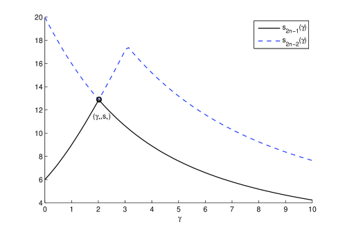
Fig 1: The singular values $s_{2n-1}(F[P(\mu);\gamma])$ (solid line) and $s_{2n-2}(F[P(\mu);\gamma])$ (dashed line).

In Figure 1, the graphs of

$$s_{2n-1}(F[P(\mu);\gamma])=s_{5}(F[P(-4);\gamma])\;\;\;\,\mbox{and}\;\;\;\,s_{2n-2}(F[P(\mu);\gamma])=s_{4}(F[P(-4);\gamma])$$

are plotted for $\gamma\in\left[{0,10}\right]$, and their common point $(\gamma_{*},s_{*})=(2.0180,12.8841)$ is marked with “$\circ$”. With respect to the discussion in the previous section, it is worth noting that in this example, the graph of $s_{2,2}(\gamma)$ (that is, $s_{n-1,2}(\gamma)$) is the graph of the decreasing functions $s_{1,2}(\gamma)$ and $s_{2,2}(\gamma)$ that intersects first the graph of the increasing function $s_{3,1}(\gamma)$ (that is, $s_{n,1}(\gamma)$). Moreover, it is apparent that $s_{2n-1}(F[P(\mu);\gamma])$ and $s_{2n-2}(F[P(\mu);\gamma])$ are non-differentiable functions at $\gamma_{*}$.

Since $s_{*}=s_{5}(F[P(-4);2.0180])=s_{4}(F[P(-4);2.0180])=12.8841$ is a double singular value, the pairs of unit vectors $\left[{\begin{array}[]{*{20}c}u_{1}(\gamma_{*})\\ u_{2}(\gamma_{*})\\ \end{array}}\right],\left[{\begin{array}[]{*{20}c}{\hat{u}_{1}(\gamma_{*})}\\ {\hat{u}_{2}(\gamma_{*})}\end{array}}\right]$ and $\left[{\begin{array}[]{*{20}c}v_{1}(\gamma_{*})\\ v_{2}(\gamma_{*})\\ \end{array}}\right],\left[{\begin{array}[]{*{20}c}{\hat{v}_{1}(\gamma_{*})}\\ {\hat{v}_{2}(\gamma_{*})}\end{array}}\right]$ form orthonormal bases of the left and right singular subspaces corresponding to $s_{*}$, respectively. So, recalling that in Lemma 2.3, assertion (1) yields assertion (2), henceforth we are looking for a pair of unit vectors

$$\left[{\begin{array}[]{*{20}c}{\tilde{u}_{1}(\gamma_{*})}\\ {\tilde{u}_{2}(\gamma_{*})}\end{array}}\right]=\alpha\left[{\begin{array}[]{*{20}c}u_{1}(\gamma_{*})\\ u_{2}(\gamma_{*})\end{array}}\right]+\beta\left[{\begin{array}[]{*{20}c}\hat{u}_{1}(\gamma_{*})\\ \hat{u}_{2}(\gamma_{*})\end{array}}\right],\;\;\left[{\begin{array}[]{*{20}c}\tilde{v}_{1}(\gamma_{*})\\ \tilde{v}_{2}(\gamma_{*})\end{array}}\right]=\alpha\left[{\begin{array}[]{*{20}c}v_{1}(\gamma_{*})\\ v_{2}(\gamma_{*})\end{array}}\right]+\beta\left[{\begin{array}[]{*{20}c}\hat{v}_{1}(\gamma_{*})\\ \hat{v}_{2}(\gamma_{*})\end{array}}\right]$$ (11)

such that

$$\tilde{u}_{2}({\gamma_{*}})^{*}P^{\prime}(\mu)\tilde{v}_{1}({\gamma_{*}})=0,$$ (12)

where the scalars $\alpha,\beta\in\mathbb{C}$ satisfy $\left|\alpha\right|^{2}+\left|\beta\right|^{2}=1$. By substituting the unknown singular vectors of (11) into (12), we obtain

$$\left[{\begin{array}[]{*{20}{c}}\overline{\alpha}&\overline{\beta}\end{array}}\right]\,M\,\left[{\begin{array}[]{*{20}{c}}\alpha\\ \beta\end{array}}\right]=0,$$ (13)

where

$$M=\left[{\begin{array}[]{*{20}{c}}u_{2}({\gamma_{*}})^{*}P^{\prime}(\mu)v_{1}({\gamma_{*}})&u_{2}({\gamma_{*}})^{*}P^{\prime}(\mu)\hat{v}_{1}({\gamma_{*}})\\ \hat{u}_{2}({\gamma_{*}})^{*}P^{\prime}(\mu)v_{1}({\gamma_{*}})&\hat{u}_{2}({\gamma_{*}})^{*}P^{\prime}(\mu)\hat{v}_{1}({\gamma_{*}})\end{array}}\right].$$ (14)

Lemma 4.1.

The matrix $M$ in (14) is always hermitian.

Proof.

Recall that $\gamma_{*}$ and $s_{*}$ are positive. By the proof of Lemma 17 in [15], it follows that the diagonal entries of matrix $M$ are real.

By the definition of the pairs of singular vectors

$$\left[{\begin{array}[]{*{20}c}{u_{1}(\gamma_{*})}\\ {u_{2}(\gamma_{*})}\\ \end{array}}\right],\left[{\begin{array}[]{*{20}c}{v_{1}(\gamma_{*})}\\ {v_{2}(\gamma_{*})}\\ \end{array}}\right]\;\;\;\mbox{and}\;\;\;\left[{\begin{array}[]{*{20}c}{\hat{u}_{1}(\gamma_{*})}\\ {\hat{u}_{2}(\gamma_{*})}\\ \end{array}}\right],\left[{\begin{array}[]{*{20}c}{\hat{v}_{1}(\gamma_{*})}\\ {\hat{v}_{2}(\gamma_{*})}\\ \end{array}}\right]$$

of $F[P(\mu);\gamma_{*}]$ corresponding to $s_{*}$, we have

$$\left\{{\begin{array}[]{*{20}c}{\left[{\begin{array}[]{*{20}c}{P(\mu)}&0\\ {\gamma_{*}P^{\prime}(\mu)}&{P(\mu)}\\ \end{array}}\right]\left[{\begin{array}[]{*{20}c}{v_{1}(\gamma_{*})}\\ {v_{2}(\gamma_{*})}\\ \end{array}}\right]=s_{*}\left[{\begin{array}[]{*{20}c}{u_{1}(\gamma_{*})}\\ {u_{2}(\gamma_{*})}\\ \end{array}}\right],}\\ {\left[{\begin{array}[]{*{20}c}{P(\mu)}&0\\ {\gamma_{*}P^{\prime}(\mu)}&{P(\mu)}\\ \end{array}}\right]\left[{\begin{array}[]{*{20}c}{\hat{v}_{1}(\gamma_{*})}\\ {\hat{v}_{2}(\gamma_{*})}\\ \end{array}}\right]=s_{*}\left[{\begin{array}[]{*{20}c}{\hat{u}_{1}(\gamma_{*})}\\ {\hat{u}_{2}(\gamma_{*})}\\ \end{array}}\right],}\\ \end{array}}\right.$$

or equivalently,

$$\left\{{\begin{array}[]{*{20}l}{P(\mu)v_{1}(\gamma_{*})=s_{*}u_{1}(\gamma_{*}),}\\ {\gamma_{*}P^{\prime}(\mu)v_{1}(\gamma_{*})+P(\mu)v_{2}(\gamma_{*})=s_{*}u_{2}(\gamma_{*}),}\\ {P(\mu)\hat{v}_{1}(\gamma_{*})=s_{*}\hat{u}_{1}(\gamma_{*}),}\\ {\gamma_{*}P^{\prime}(\mu)\hat{v}_{1}(\gamma_{*})+P(\mu)\hat{v}_{2}(\gamma_{*})=s_{*}\hat{u}_{2}(\gamma_{*}),}\end{array}}\right.$$ (15)

and

$$\left\{{\begin{array}[]{*{20}c}{\left[{\begin{array}[]{*{20}c}{u_{1}(\gamma_{*})^{*}}&{u_{2}(\gamma_{*})^{*}}\\ \end{array}}\right]\left[{\begin{array}[]{*{20}c}{P(\mu)}&0\\ {\gamma_{*}P^{\prime}(\mu)}&{P(\mu)}\\ \end{array}}\right]=s_{*}\left[{\begin{array}[]{*{20}c}{v_{1}(\gamma_{*})^{*}}&{v_{2}(\gamma_{*})^{*}}\\ \end{array}}\right],}\\ {\left[{\begin{array}[]{*{20}c}{\hat{u}_{1}(\gamma_{*})^{*}}&{\hat{u}_{2}(\gamma_{*})^{*}}\\ \end{array}}\right]\left[{\begin{array}[]{*{20}c}{P(\mu)}&0\\ {\gamma_{*}P^{\prime}(\mu)}&{P(\mu)}\\ \end{array}}\right]=s_{*}\left[{\begin{array}[]{*{20}c}{\hat{v}_{1}(\gamma_{*})^{*}}&{\hat{v}_{2}(\gamma_{*})^{*}}\\ \end{array}}\right],}\\ \end{array}}\right.$$

or equivalently,

$$\left\{{\begin{array}[]{*{20}l}{u_{1}(\gamma_{*})^{*}P(\mu)+\gamma_{*}u_{2}(\gamma_{*})^{*}P^{\prime}(\mu)=s_{*}v_{1}(\gamma_{*})^{*},}\\ {u_{2}(\gamma_{*})^{*}P(\mu)=s_{*}v_{2}(\gamma_{*})^{*},}\\ {\hat{u}_{1}(\gamma_{*})^{*}P(\mu)+\gamma_{*}\hat{u}_{2}(\gamma_{*})^{*}P^{\prime}(\mu)=s_{*}\hat{v}_{1}(\gamma_{*})^{*},}\\ {\hat{u}_{2}(\gamma_{*})^{*}P(\mu)=s_{*}\hat{v}_{2}(\gamma_{*})^{*}.}\end{array}}\right.$$ (16)

By multiplying the fourth equation in (15) by $u_{2}(\gamma_{*})^{*}$ from the left, and the second equation of (16) by $\hat{v}_{2}(\gamma_{*})$ from the right, we obtain

$$\gamma_{*}u_{2}(\gamma_{*})^{*}P^{\prime}(\mu)\hat{v}_{1}(\gamma_{*})+u_{2}(\gamma_{*})^{*}P(\mu)\hat{v}_{2}(\gamma_{*})=s_{*}u_{2}(\gamma_{*})^{*}\hat{u}_{2}(\gamma_{*}),$$ (17)

and

$$u_{2}(\gamma_{*})^{*}P(\mu)\hat{v}_{2}(\gamma_{*})=s_{*}v_{2}(\gamma_{*})^{*}\hat{v}_{2}(\gamma_{*}),$$ (18)

respectively. As a consequence,

$$\gamma_{*}u_{2}(\gamma_{*})^{*}P^{\prime}(\mu)\hat{v}_{1}(\gamma_{*})=s_{*}\left({u_{2}(\gamma_{*})^{*}\hat{u}_{2}(\gamma_{*})-v_{2}(\gamma_{*})^{*}\hat{v}_{2}(\gamma_{*})}\right).$$ (19)

Performing similar calculations, one can verify that

$$\gamma_{*}\hat{u}_{2}(\gamma_{*})^{*}P^{\prime}(\mu)v_{1}(\gamma_{*})=s_{*}\left({\hat{u}_{2}(\gamma_{*})^{*}u_{2}(\gamma_{*})-\hat{v}_{2}(\gamma_{*})^{*}v_{2}(\gamma_{*})}\right).$$ (20)

Clearly, equations (19) and (20) imply that the non-diagonal entries of matrix $M$ are complex conjugate. ∎

By Lemma 2.3 (1), equation (13) has always a nontrivial (i.e., nonzero) solution, and hence, the hermitian matrix $M$ in (14) cannot be (positive or negative) definite. In our numerical example, $M$ has a negative and a positive diagonal entries (namely, $-2.6396$ and $4.1089$), and thus, it is an indefinite hermitian matrix.

To derive an explicit solution of (13), suppose that $\eta_{1},\eta_{2}\in\mathbb{C}$ are the (real) eigenvalues of matrix $M$, with $\eta_{1}>0>\eta_{2}$, and let $w_{1},w_{2}\in\mathbb{C}^{2}$ be unit eigenvectors of $M$ corresponding to $\eta_{1}$ and $\eta_{2}$, respectively. Then, it is straightforward to see (keeping in mind the orthogonality of the eigenvectors) that the unit vector

$$\left[{\begin{array}[]{*{20}{c}}\alpha\\ \beta\end{array}}\right]=\sqrt{\frac{\left|\eta_{2}\right|}{\left|\eta_{1}\right|+\left|\eta_{2}\right|}}\,w_{1}+\sqrt{\frac{\left|\eta_{1}\right|}{\left|\eta_{1}\right|+\left|\eta_{2}\right|}}\,w_{2}$$

satisfies

$$\left[{\begin{array}[]{*{20}{c}}\overline{\alpha}&\overline{\beta}\end{array}}\right]\,M\,\left[{\begin{array}[]{*{20}{c}}\alpha\\ \beta\end{array}}\right]=\frac{\left|\eta_{1}\right|\eta_{2}}{\left|\eta_{1}\right|+\left|\eta_{2}\right|}+\frac{\left|\eta_{2}\right|\eta_{1}}{\left|\eta_{1}\right|+\left|\eta_{2}\right|}=0.$$

Finally, in order to verify the validity of this refinement, we return again to the normal matrix polynomial $P(\lambda)$ in (5), and by applying the above methodology, we obtain $\alpha=0.6254$ and $\beta=0.7803$. Consequently, the desired vectors in (11) are (approximately)

$$\left[{\begin{array}[]{*{20}c}{\tilde{u}_{1}(\gamma_{*})}\\ {\tilde{u}_{2}(\gamma_{*})}\end{array}}\right]=\left[\begin{array}[]{c}0\\ 0.6560\\ -0.2640\\ 0\\ 0.4226\\ 0.5669\end{array}\right]\;\;\;\mbox{and}\;\;\;\left[{\begin{array}[]{*{20}c}{\tilde{v}_{1}(\gamma_{*})}\\ {\tilde{v}_{2}(\gamma_{*})}\end{array}}\right]=\left[\begin{array}[]{c}0\\ 0.4226\\ -0.5669\\ 0\\ 0.6560\\ 0.2640\end{array}\right].$$

In particular, it holds that

$$\tilde{u}_{2}^{*}({\gamma_{*}})P^{\prime}(-4)\tilde{v}_{1}({\gamma_{*}})=-4.4409\cdot 10^{-16},$$

and for the $n\times 2$ matrices $\tilde{U}(\gamma_{*})=\left[\tilde{u}_{1}(\gamma_{*})~{}\tilde{u}_{2}(\gamma_{*})\right]$ and $\tilde{V}(\gamma_{*})=\left[\tilde{v}_{1}(\gamma_{*})~{}\tilde{v}_{2}(\gamma_{*})\right]$, we have

$$\left\|\tilde{U}^{*}({\gamma_{*}})\tilde{U}({\gamma_{*}})-\tilde{V}^{*}({\gamma_{*}})\tilde{V}({\gamma_{*}})\right\|_{2}=1.1383\cdot 10^{-6}.$$

Thus, Lemma 2.3 is verified.

Moreover, using the matrices $\tilde{U}({\gamma_{*}})$ and $\tilde{V}({\gamma_{*}})$, Theorem 2.4 yields the upper bound $0.9465$ for the distance from $P(\lambda)$ to the set of $3\times 3$ quadratic matrix polynomials that have $\mu=-4$ as a multiple eigenvalue, and the perturbed matrix polynomial

$${\tilde{Q}_{{\gamma_{*}}}}(\lambda)=\left[{\begin{array}[]{*{20}{c}}1&0&0\\ 0&{0.0680}&{0.0152}\\ 0&{-0.1552}&{0.5986}\end{array}}\right]{\lambda^{2}}+\left[{\begin{array}[]{*{20}{c}}{-3}&0&0\\ 0&{-0.0680}&{-0.0152}\\ 0&{0.1552}&{3.4014}\end{array}}\right]\lambda+\left[{\begin{array}[]{*{20}{c}}2&0&0\\ 0&{-0.9320}&{0.0152}\\ 0&{-0.1552}&{1.5986}\end{array}}\right]$$

that lies on the boundary of $\,\mathcal{B}\left(P,0.9465,\textup{w}\right)$ and has spectrum

$$\sigma\left(\tilde{Q}_{{\gamma_{*}}}(\lambda)\right)=\left\{1,\,2,\,4.1982,\,-0.5140,\,-4.0000+\textup{i}\,0.0031,\,-4.0000-\textup{i}\,0.0031\right\}.$$

In addition, the lower bound $0.4031$ of the distance is given by Theorem 11 in [15]. (All computations were performed in Matlab with $16$ significant digits.)

4.2 The case of multiplicity greater than 2

Suppose that $\gamma_{*}>0$, and the multiplicity of the singular value $s_{*}>0$ is $r\geq 3$. For weakly normal matrix polynomials, this means that the graph of the increasing function $s_{n,1}(\gamma)$ intersects the graphs of more than one of the $n-1$ decreasing functions $s_{1,2}(\gamma),s_{2,2}(\gamma),\dots,s_{n-1,2}(\gamma)$, at the point $(\gamma_{*},s_{*})$.

Let also

$$\left[{\begin{array}[]{*{20}c}u_{1}^{(1)}(\gamma_{*})\\ u_{2}^{(1)}(\gamma_{*})\end{array}}\right],\,\left[{\begin{array}[]{*{20}c}u_{1}^{(2)}(\gamma_{*})\\ u_{2}^{(2)}(\gamma_{*})\end{array}}\right],\,\dots,\,\left[{\begin{array}[]{*{20}c}u_{1}^{(r)}(\gamma_{*})\\ u_{2}^{(r)}(\gamma_{*})\end{array}}\right]$$

and

$$\left[{\begin{array}[]{*{20}c}v_{1}^{(1)}(\gamma_{*})\\ v_{2}^{(1)}(\gamma_{*})\end{array}}\right],\,\left[{\begin{array}[]{*{20}c}v_{1}^{(2)}(\gamma_{*})\\ v_{2}^{(2)}(\gamma_{*})\end{array}}\right],\,\dots,\,\left[{\begin{array}[]{*{20}c}v_{1}^{(r)}(\gamma_{*})\\ v_{2}^{(r)}(\gamma_{*})\end{array}}\right]$$

be orthonormal bases of the left and right singular subspaces of $F[P(\mu);\gamma_{*}]$ corresponding to $s_{*}$, respectively. Then, we are looking for a pair of unit vectors

$$\left[{\begin{array}[]{*{20}c}{\tilde{u}_{1}(\gamma_{*})}\\ {\tilde{u}_{2}(\gamma_{*})}\end{array}}\right]=\sum_{j=1}^{r}\alpha_{j}\left[{\begin{array}[]{*{20}c}u_{1}^{(j)}(\gamma_{*})\\ u_{2}^{(j)}(\gamma_{*})\end{array}}\right],\;\;\left[{\begin{array}[]{*{20}c}\tilde{v}_{1}(\gamma_{*})\\ \tilde{v}_{2}(\gamma_{*})\end{array}}\right]=\sum_{j=1}^{r}\alpha_{j}\left[{\begin{array}[]{*{20}c}v_{1}^{(j)}(\gamma_{*})\\ v_{2}^{(j)}(\gamma_{*})\end{array}}\right]$$ (21)

such that

$$\tilde{u}_{2}({\gamma_{*}})^{*}P^{\prime}(\mu)\tilde{v}_{1}({\gamma_{*}})=0,$$ (22)

where the scalars $\alpha_{1},\alpha_{2},\dots,\alpha_{r}\in\mathbb{C}$ satisfy $\left|\alpha_{1}\right|^{2}+\left|\alpha_{2}\right|^{2}+\cdots+\left|\alpha_{r}\right|^{2}=1$.

Following the arguments of the methodology described in the previous subsection, we can compute the desired vectors in (21) that satisfy (22). In particular, we need to find a solution of the equation

$$\left[{\begin{array}[]{*{20}{cccc}}\overline{\alpha}_{1}&\overline{\alpha}_{2}&\cdots&\overline{\alpha}_{r}\end{array}}\right]\,M_{r}\,\left[{\begin{array}[]{*{20}{c}}\alpha_{1}\\ \alpha_{2}\\ \vdots\\ \alpha_{r}\end{array}}\right]=0,$$ (23)

where the $r\times r$ matrix

$$M_{r}=\left[{\begin{array}[]{*{20}{cccc}}u_{2}^{(1)}({\gamma_{*}})^{*}P^{\prime}(\mu)v_{1}^{(1)}({\gamma_{*}})&u_{2}^{(1)}({\gamma_{*}})^{*}P^{\prime}(\mu)v_{1}^{(2)}({\gamma_{*}})&\cdots&u_{2}^{(1)}({\gamma_{*}})^{*}P^{\prime}(\mu)v_{1}^{(r)}({\gamma_{*}})\\ u_{2}^{(2)}({\gamma_{*}})^{*}P^{\prime}(\mu)v_{1}^{(1)}({\gamma_{*}})&u_{2}^{(2)}({\gamma_{*}})^{*}P^{\prime}(\mu)v_{1}^{(2)}({\gamma_{*}})&\cdots&u_{2}^{(2)}({\gamma_{*}})^{*}P^{\prime}(\mu)v_{1}^{(r)}({\gamma_{*}})\\ \vdots&\vdots&\ddots&\vdots\\ u_{2}^{(r)}({\gamma_{*}})^{*}P^{\prime}(\mu)v_{1}^{(1)}({\gamma_{*}})&u_{2}^{(r)}({\gamma_{*}})^{*}P^{\prime}(\mu)v_{1}^{(2)}({\gamma_{*}})&\cdots&u_{2}^{(r)}({\gamma_{*}})^{*}P^{\prime}(\mu)v_{1}^{(r)}({\gamma_{*}})\\ \end{array}}\right]$$

is hermitian and not definite. Considering a unit eigenvector $w_{\max}\in\mathbb{C}^{r}$ of $M_{r}$ corresponding to the maximum eigenvalue $\eta_{\max}>0$ of $M_{r}$ and an eigenvector $w_{\min}\in\mathbb{C}^{r}$ corresponding to the minimum eigenvalue $\eta_{\min}<0$ of $M_{r}$, it is straightforward to verify that the unit vector

$$\sqrt{\frac{\left|\eta_{\min}\right|}{\left|\eta_{\max}\right|+\left|\eta_{\min}\right|}}\,w_{\max}+\sqrt{\frac{\left|\eta_{\max}\right|}{\left|\eta_{\max}\right|+\left|\eta_{\min}\right|}}\,w_{\min}$$

satisfies (23).