On the use of the index N2 to derive the metallicity in metal-poor galaxies

Abstract

The N2 index ([Nii]$\rm\lambda$6584/H$\rm\alpha$) is used to determine emission line galaxy metallicities at all redshifts, including high redshift, where galaxies tend to be metal-poor. The initial aim of the work was to improve the calibrations used to infer oxygen abundance from N2 employing updated low-metallicity galaxy databases. We compare N2 and the metallicity determined using the direct method for the set of extremely metal-poor galaxies compiled by Morales-Luis et al. (2011). To our surprise, the oxygen abundance presents a tendency to be constant with N2, with a very large scatter. Consequently, we find that the existing N2 calibrators overstimate the oxygen abundance for most low metallicity galaxies, and then they can be used only to set upper limits to the true metallicity in low-metallicity galaxies. An explicit expression for this limit is given. In addition, we try to explain the observed scatter using photoionization models. It is mostly due to the different evolutionary state of the Hii regions producing the emission lines, but it also arises due to differences of N/O among the galaxies.

1. Introduction

Optical bright emission lines have been used for many years as the main source of information to derive physical properties and chemical abundances both in nearby and distant galaxies. These optical emission-lines are excited by the UV radiation emitted by young massive stars in the gas clouds surrounding on-going star-formation complexes in galaxies. The total metallicity ($\rm Z$) of the gas-phase is one of the most relevant pieces of information that can be extracted. In particular, the regime of low metallicity is particularly important in the context of unevolved/young objects resembling the first protogalaxies (e.g., Izotov et al. 2006; Morales-Luis et al. 2011) and or star-formation in the high redshift universe (e.g., Cresci et al. 2010; Mannucci et al. 2011; Troncoso et al. 2014).

The most accurate method to derive $\rm Z$ using the bright collisionally excited emission-lines is the determination of the total oxygen abundance; O/H based on measuring the electron temperature, the so-called $\rm T_{e}$ method. $\rm T_{e}$ can be derived from the ratio of lines with different excitation potential; the most widely used is the ratio of oxygen lines, [Oiii]$\lambda$4363/([Oiii]$\lambda 4959+$ [Oiii]$\lambda 5007$). Then, the ionic abundances of the most abundant oxygen ions is obtained from the ratio of their brightest emission-lines to a Hydrogen Balmer line, i.e., [Oii]$\lambda$3727/H$\beta$ for O⁺ and [Oiii]$\lambda$5007/H$\beta$ for O²⁺ (e.g., Pagel et al. 1992; Hägele et al. 2008).

Unfortunately, the $\rm T_{e}$ method is often useless at large redshifts due to the faintness of the weak auroral lines and/or because the wavelength coverage does not include the emission-lines required to derive of the observation electron temperature or ionic abundances. In those cases, other methods based only on the brightest available emission-lines are used instead. One of the most popular ones is based on the ratio between [Nii]$\lambda$6584 and H$\alpha$, the so-called N2 parameter (e.g., Storchi-Bergmann et al. 1994; Denicoló et al. 2002; Pettini & Pagel 2004; Pérez-Montero & Contini 2009). This parameter involves emission lines close in wavelength so it is almost independent of reddening or flux calibration uncertainties. N2 presents a linear relation with log(O/H), within a range of metallicity including extremely metal poor (XMP) galaxies (e.g., Denicoló et al. 2002; Pettini & Pagel 2004; Pérez-Montero & Contini 2009; López-Sánchez et al. 2012; Marino et al. 2013). Moreover, N2 allows measuring O/H in high redshift objects, because the required [Nii] emission-line appears in many high-z surveys focused on the detection of H$\alpha$ in near-IR bands (e.g., Erb 2008; Queyrel et al. 2009, 2012). Other methods widely used to derive O/H based on strong collisional emission lines have revealed to be quite inefficient in the range of XMPs. For instance, the R23 parameter (Pagel et al. 1979) has a bi-valuated behaviour with O/H in high redshift objects, and O3N2 (Alloin et al. 1979) cannot be used for oxygen abundance 12+log(O/H)$<$8 (e.g., Marino et al. 2013).

This paper is focused on the empirical O/H estimate using the N2 index in metal-poor galaxies. We wanted to take advantage of the comprehensive sample of metal-poor galaxies compiled by Morales-Luis et al. (2011) to improve the significance of the calibrations O/H versus N2 obtained so far (e.g. Denicoló et al. 2002; Pettini & Pagel 2004; Nagao et al. 2006; Pérez-Montero & Contini 2009). To our surprise, we found that the scatter of the relationship O/H versus N2 increases when improving the statistics, and reveals that the ratio [Nii]$\lambda$6583 to H$\alpha$ seems to be independent of metallicity at low oxygen abundance (12+log(O/H)$<$7.6, which corresponds to a metallicity $\rm Z\lesssim Z_{\odot}/10$). This result casts doubts on the metallicities of high-redshift metal-poor objects based on N2, but indicates that N2 can be used to set an upper limit to the true metallicity of the targets. This paper describes the problem, the solution, and explains how the behaviour of N2 can be understood using photoionization models.

The paper is organized as follows. First, we describe the sample of 46 XMP galaxies (Section 2) used to calibrate the N2-based empirical metallicity estimate. The $\rm T_{e}$ method we use to determine physical properties and chemical abundances is presented in Section 3. The $\rm T_{e}$ method is employed to determine the chemical abundances of the sample of XMPs in Section 4. In order to identify the sources of scatter in the N2 calibration at low metallicities, photoionization models are analyzed in Section 5.1. The sources of the observed scatter are identified in Section 5.2. A summary with conclusions and follow-up work is provided in Section 6.

2. Extremely Metal Poor galaxy sample

In order to calibrate the index N2 in the very low-Z range, we need a large sample of low-Z targets with their O/H homogeneously determined via the direct method.

We start off from the metal-poor galaxy sample compiled by Morales-Luis et al. (2011), which included all galaxies with metallicity one tenth or less of the solar value (i.e., 12 + log(O/H)$<$7.69, Asplund et al. 2009) found to the date of publication. The total sample includes 140 XMPs. Among them, 79 have spectra in SDSS/DR7, which is the spectral database used in the calibration.

Nearby galaxies with spectra in SDSS (objects with $\rm redshift\lesssim 0.024$) have [Oii]$\lambda$3727 out of the observed spectral range, thus the determination of the $\rm O^{+}/H^{+}$ by the direct method, i.e., using [Oii]$\lambda$3727, is not possible. A slight modification of the direct method allows to calculate the value of $\rm O^{+}/H^{+}$ from the intensities of the auroral lines [Oii]$\lambda\lambda$7320,7330 (Aller 1984) and was explored. It is important, however, to bear in mind that the application of the auroral line method is restricted to spectra with sufficiently high signal-to-noise ratio (Kniazev et al. 2004). Because of this, we select galaxies with S/N $\gtrsim$ 3 in [Oii]$\lambda$7320. Only 31 of the 79 metal-poor galaxies with SDSS spectra fulfill the required S/N criterion. We added 15 galaxies to the sample taking into account the similarity between N and O ionization structures. With N/O obtained using the N2S2 index (Pérez-Montero & Contini 2009) and $\rm N^{+}/H^{+}$ inferred through the functional form by Hägele et al. (2008), it is possible to estimate $\rm O^{+}/H^{+}$ when [Oii] lines are unavailable. In summary, we have 46 XMP galaxies with their metallicities determined in a homogeneous and consistent way, which is the main sample employed in this paper.

In order to put our work into context, we also randomly select and analyze a control sample of 65 starburst galaxies, having intermediate metallicities ($\rm 7.7\leq 12+log(O/H)\leq 8.2$). We first select those emission line galaxies in SDSS/DR7 which were not classified as metal-poor galaxies by Morales-Luis et al. (2011). Then, we discarded AGNs using the BPT diagram (Baldwin et al. 1981). Finally, we divided the range of N2 roughly corresponding to $\rm 7.7\leq 12+log(O/H)\leq 8.2$ in 65 equal intervals, and then one galaxy was randomly selected per interval.

3. Technique to derive the physical properties and chemical abundances

The emission-line fluxes of the spectra of the 46 XMPs and the 65 galaxies in the control sample are measured using our own IDL procedure to better control the errors and their propagation. Basically, the procedure works as the task SPLOT in IRAF. In the case of an isolated line or two blended unresolved lines, they are measured integrating between two points given by the position of the local continuum identified by eye. If two lines are blended, but they can be resolved, we use a multiple Gaussian fit to estimate individual fluxes.

The statistical error associated with the observed emission lines is calculated using the expression $\rm\sigma_{1}=\sigma_{c}N^{1/2}[1+EW/(N\Delta)]^{1/2}$ (Gonzalez-Delgado et al. 1994; Castellanos et al. 2002; Pérez-Montero & Díaz 2003), where $\rm\sigma_{1}$ is the error in the observed line flux, $\rm\sigma_{c}$ corresponds to the noise in the continuum near the measured emission line, $\rm N$ is the number of pixels used in the measurement of the line flux, $\rm EW$ is the line equivalent width, and $\rm\Delta$ is the wavelength dispersion.

All line fluxes were corrected for reddening using the same procedures as in Hägele et al. (2008). The reddening coefficient in H$\rm\beta$, $\rm c(H\beta)$, was calculated assuming the extinction law of Miller & Mathews (1972) for the Galaxy and performing a least-squares fit to the difference between the theoretical and observed Balmer decrement. The corrected emission line flux of a line with wavelength $\rm\lambda$, $\rm I(\lambda)$, is given by

$$\rm\frac{I(\lambda)}{I(H\beta)}=\frac{F(\lambda)}{F(H\beta)}\cdot 10^{c(H\beta)f(\lambda)},$$ (1)

where $\rm F(\lambda)$ stands for the measured emission line flux, and $\rm f(\lambda)$ is the extinction law at the corresponding wavelength.

With the reddening corrected fluxes, we determine the physical conditions of the ionized gas, electron temperature and electron density included. Electron temperature and electron density determinations are based on the five-level statistical equilibrium atom approximation in the task TEMDEN of IRAF (De Robertis et al. 1987). Electron density is derived from the ratio [Sii]$\lambda$6717/[Sii]$\lambda$6731, and in objects without this ratio, a density of 100 $\rm cm^{-3}$ is assumed, typical in this kind of galaxies (e.g. Pérez-Montero & Díaz 2005). The electron temperature of [Oiii] is derived using the ratio ([Oiii]$\lambda$4959+[Oiii]$\lambda$5007)/[Oiii]$\lambda$4363 (e.g., Stasińska 2004).

As we mentioned in Sec. 2, [Oii]$\lambda$3727 is often out of the wavelength range in the SDSS spectra of our galaxies, thus the electron temperature of [Oii] is calculated using the model relation between t([Oii]) and t([Oiii]) worked out by Pérez-Montero & Díaz (2003). Furthermore, in the 15 cases without $\rm O^{+}/H^{+}$, we need the electron temperature of [Nii] to calculate $\rm N^{+}/H^{+}$. t[Nii]) can be derived from the emission-line ratio ([Nii]$\lambda$6584 +[Nii]$\lambda$6548)/[Nii]$\lambda$5755 in 8 objects. The remaining 7 cases use an independent relation between t([Nii]) and t([Oiii]) worked out by Pérez-Montero & Contini (2009).

This particular study uses oxygen abundance to trace the metallicity, therefore, we have not calculated the abundance of other elements. The measures calculates the total oxygen abundance relative to hydrogen using,

$$\rm\frac{O}{H}\backsimeq\frac{O^{+}+O^{2+}}{H^{+}}.$$ (2)

The ionic abundances of $\rm O^{+}$ and $\rm O^{2+}$ are obtained employing the expressions given by Hägele et al. (2008), which consider the lines [Oiii]$\rm\lambda$4959 and [Oiii]$\rm\lambda$5007 for $\rm O^{2+}$, and [Oii]$\rm\lambda\lambda$7320,7330 for $\rm O^{+}$. O³⁺ does not need to be included since its abundance is negligibly small in Hii regions (e.g., Stasińska et al. 2012; Andrews & Martini 2013). For those galaxies without a direct determination of the ionic abundance $\rm O^{+}/H^{+}$, considering the similarity of ionization structures of N and O, it is possible to assume,

$$\rm\frac{N}{O}\backsimeq\frac{N^{+}}{O^{+}}.$$ (3)

With N/O obtained using the N2S2 index by Pérez-Montero & Contini (2009), and $\rm N^{+}/H^{+}$, calculated employing the approximation by Hägele et al. (2008), it is possible to determine $\rm O^{+}/H^{+}$ through the expression,

$$\rm\frac{O^{+}}{H^{+}}=\frac{N^{+}}{H^{+}}\frac{O}{N}.$$ (4)

Errors in chemical abundances and physical properties are estimated in a Montecarlo simulation. The line fluxes involved in determining the physical conditions and chemical abundances are randomly modified 500 times according to their observed errors, and the abundances are computed for each one of these realizations. The error for the abundance is the standard deviation among all the values thus obtained. The noise added to the observed fluxes is assumed to be Gaussian. These error bars do not include systematic errors, which may be non-negligible. For instante, even XMP galaxias, where the dust is almost absent (e.g., Fisher et al. 2014), may have 20% of their O depleted into dust grains (e.g., Peimbert & Peimbert 2010). This represent an artificial drop of metallicity of 0.08 dex. Similar error results from ignoring temperature inhomogenities (e.g., Peimbert & Peimbert 2010).

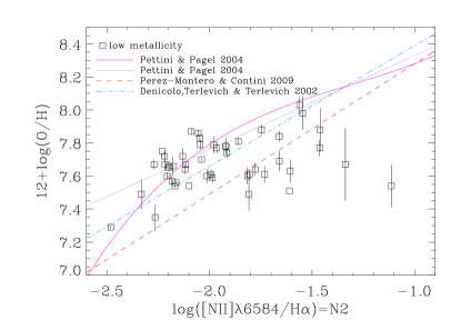
Figure 1.— Oxygen abundance versus N2 for the XMP galaxy sample. We also include the third-order polynomial calibration of the relationship from PP04 (the solid line), the linear fit calibration from PP04 (the dash triple-dot line), the linear calibration from Pérez-Montero & Contini (2009) (the dashed-line) and the linear calibration from Denicoló et al. (2002) (the dash-dot line).

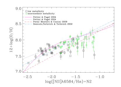
Figure 2.— Oxygen abundance versus N2 for the full sample, i.e., the low metallicity sample (the black squares) plus the control sample (the green diamonds). We also include the third-order polynomial calibration from PP04 (the solid line), the linear fit calibration from PP04 (the dash triple-dot line), the linear calibration from Pérez-Montero & Contini (2009) (the dashed-line) and the linear calibration from Denicoló et al. (2002) (the dash-dot line). The lines represent typical calibrations used in the literature to derive O/H from N2.

4. Metallicity and N2 index

The oxygen nebular metallicity computed for the metal-poor sample is compared with N2 in Fig. 1. The first important result is that, most of the galaxies have metallicities one tenth or less of the solar value. Therefore, the oxygen abundance obtained using the direct method confirms that most galaxies selected as low-metallicity galaxies in Morales-Luis et al. (2011) are, indeed, XMPs.

In addition, the observed oxygen abundance presents a tendency to be constant with N2 for the metal-poor galaxies, i.e., metallicities have similar values for a broad range of [Nii]$\lambda 6583$/H$\alpha$ (Fig. 1). This is discouraging if one tries to use N2 as proxy for metallicity at low metallicity. As we argue below, N2-based metallicity estimates by Pettini & Pagel (2004, PP04) calibrate the N2 index versus O/H relationship in the range $\rm 7\leq 12+log(O/H)\leq 8.7$ (see Fig. 1). The data set used by PP04 presents a discontinuity in metallicity in the region of XMP galaxies. Figure 2 shows our metal-poor galaxy sample together with the control sample. There is no jump in the low metallicity range. Then, we conclude that the apparent discontinuity in PP04 is due to the small number of data points they had available. The present sample makes use of a more recent and larger database and, the oxygen abundance versus N2 shows a continuous trend even in the low metallicity range.

The scatter of the relationship $\rm\log(O/H)$ vs N2 is very large (Fig. 2). This scatter is also present in other samples like the one used by Pettini & Pagel (2004) and the more recent sample analyzed by Berg et al. (2012). We initially attempted to calibrate the N2 index in the low metallicity range, but we gave up due to the scatter of the observed points. However, N2 can be safely used to set an upper limit to the true metallicity in the low metallicity range. The third-order polynomial calibration from PP04 suffices for this objective (see the fit inserted in Fig. 2), namely,

$$\rm 12+log(O/H)\lesssim 9.37+2.03\cdot N2+1.26\cdot N2^{2}+0.32\cdot N2^{3},$$ (5)

when $\rm-2.5\leq N2\leq-1$. Equation 5 grants that a XMP galaxy according to N2 is a truly XMP galaxy.

5. Origin of the scatter in the metallicity versus N2 relationship

5.1. Photoionization models

In order to understand the source of scatter in Figs. 1 and 2, we developed a set of photoionization models using CLOUDY (v.10; Ferland et al. 1998), covering the physical condition expected for the observed objects.

The photoionization models assume a spherically symmetric Hii region, with the ionized emitting gas taken to have a constant density of 50 $\rm cm^{-3}$. We also tried models with constant gas pressure, but they do not significantly modify the emission line ratios with respect to constant density models, and so this assumption does not bias the conclusions of the modeling. The models have plane-parallel geometry. The gas is ionized by a coeval cluster of massive stars, with the spectral energy distribution (SED) obtained using Starburst99 synthetic stellar atmospheres (Leitherer et al. 1999). The age of the cluster is 1 Myr. We use an initial mass function (IMF) with exponents 1.3 and 2.3 at low and high masses, respectively. Boundaries for the IMF are 0.1 and 100 $\rm M_{\odot}$, and the exponent changes at 0.5 $\rm M_{\odot}$. Models use Padova AGB stellar tracks with metallicities Z=0.004 and Z=0.0004, the latter being the lowest available metallicity. Assuming solar composition (Asplund et al. 2009), Z=0.0004 $\equiv$ 12+log(O/H)=7.16 and Z=0.004 $\equiv$ 12+log(O/H)=8.16, which corresponds to the range of oxygen abundance found in our targets.

Figure 3.— log(N/O) versus 12+log(O/H) for the metal-poor galaxy sample using N2S2 from Pérez-Montero & Contini (2009). Error bars are calculated as is explained in Sec. 3.

The available metallicities are too coarse for the intended modeling. Therefore, for intermediate metallicity, we interpolate the two extreme spectra, one with $\rm Z_{1}=0.0004$ and the other with $\rm Z_{2}=0.004$. If

$$\rm Z=w_{1}\cdot Z_{1}+w_{2}\cdot Z_{2},$$ (6)

then the spectrum corresponding to metallicity Z, $\rm S_{Z}$, is

$$\rm S_{Z}=w_{1}\cdot S_{Z_{1}}+w_{2}\cdot S_{Z_{2}},$$ (7)

with $0<\rm w_{1},w_{2}<1$ and, $\rm w_{1}+w_{2}=1$.

It is also assumed that the gas has the same metallicity as the ionizing stars. The other ionic abundances are set in solar proportions (Asplund et al. 2009), except in the case of nitrogen, where we explore different values of N/O. Our galaxies are expected to have $\log(\rm N/O)\approx-1.6$ (Henry et al. 2000). To measure N/O one would ideally like to have [Oii]$\lambda$3727, but, as it is explained in Sec. 2, the line is often outside the observed spectral range. In this case we use N2S2 index to obtain an approximate value of N/O (Pérez-Montero & Contini 2009). Fig. 3 shows the result for our sample. From the figure we see that the metal-poor galaxies have typically $\rm-1.6\leq\log(N/O)\leq-1.4$. Taking into account this fact, we compute two sets of models with $\log(\rm N/O)=-1.6$ and $\rm-1.4$. Each one is built for a number of ionization parameters $\rm\log U=-3,-2.9,-2.7,-2.5,-2.4,-2.2,-2$ and for a number of oxygen abundances $12+\log(\rm O/H)=7.16,7.26,7.36,7.46.7.56,7.66,7.76,7.86,7.96,8.06,8.16$. The range of $\rm\log U$ corresponds to the ionization degree shown by the type of object studied here (e.g., Pérez-Montero & Díaz 2005). All in all, we have 154 photoionization models which allow us to predict N2 of a function of 12+log(O/H) under a large number of circumstances.

5.2. Scatter in $\rm O/H$ vs $\rm N2$

When looking for a metallicity indicator based on bright emission lines such as N2, one would ideally like to find combinations of lines whose fluxes depend only on chemical abundances. This is difficult because the emission line fluxes are controlled by other physical parameters as well. In the case of N2, the ionization parameter (U), i.e., ratio between the number of ionizing photons and density of hydrogen atoms, is the parameter cause most of the intrinsic variations (Denicoló et al. 2002).

In order to understand and identify the relationship between the scatter observed in Fig. 1 and the ionization parameter, we employ the photoionization models described in Sec. 5.1. [Oiii]/H$\beta$=[Oiii]$\rm(\lambda 4959+\lambda 5007)/H\beta$ weakly depends on metallicity in a non-trivial way, although it is mainly sensitive to the ionization parameter at sub-solar metallicity (e.g., Baldwin et al. 1981; Kewley et al. 2001; Levesque et al. 2010). We use the observed [Oiii]/H$\beta$ together with the models to estimate U in individual galaxies. Metallicity and N/O are known. Thereby, we plot [Oiii]/H$\beta$ versus N2 for the models and the galaxies, and we assign to each galaxy the nearest value of U. The results are shown in Fig. 4, which contains oxygen abundance versus N2 with different colors representing different ionization parameters. This plot is quite revealing, because it indicates that the scatter observed in Fig. 1 can be explained by the galaxies having different degree of ionization. As Fig. 4 shows, given an oxygen abundance, N2 decreases with increasing ionization parameter.

The degree of ionization of a galaxy changes with its evolutionary state (e.g., Levesque et al. 2010). The observed equivalent width of H$\beta$ (EW(H$\beta$)) indicates the age of the ionizing cluster (e.g., Leitherer et al. 1999), although it also depends on the underlying stellar component of the galaxies that provides most of the photons in continuum wavelengths. Pérez-Montero et al. (2010) showed that the underlying population contribution is less than 10% in a sample of Hii galaxies similar to our targets. Therefore, we can use $\rm EW(H\beta)$ as a qualitative estimate of the evolutionary state of our XMP sample. We computed EW(H$\beta$) for our galaxies, and the maximum of the distribution is at EW(H$\beta$)$\simeq$100Å. Galaxies in two different age ranges are shown in Fig. 5; the red filled circles correspond to EW(H$\beta$)$<$100Å whereas the galaxies with EW(H$\beta$)$\geq$100Å are shown as black filled circles. Lower EW(H$\beta$)s correspond to younger galaxies. Comparing Fig. 4 and 5, we can see that the galaxies with low ionization parameter are the most evolved ones. These results indicate that part of the dispersion showed in Fig. 1 is related to the evolutionary state of the galaxies through the ionization parameter U.

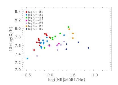
Figure 4.— Oxygen abundance versus N2 for the metal-poor galaxy sample. Each color is associated with one value of $\rm\log U$ as coded in the inset. There is a clear trend for smaller N2 to have lower U. The relationship is not one-to-one, though.

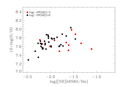
Figure 5.— Oxygen abundance versus N2 for the metal-poor galaxy sample. Red filled circles represent galaxies with EW(H$\beta$)$<$100Å, whereas black filled circles stand for galaxies with EW(H$\beta$)$\geq$100Å.

The dependence of the scatter in Fig. 1 on N/O was also explored. Since N2 uses N line to measure O abundance, ti most depend on N/O. As one can hinted at differences in Fig. 6, another source of scatter seems to be in the N/O ratio. The figure separates galaxies with log (N/O)$\leq$-1.5 (red filled circles) and galaxies with log (N/O)$>$-1.5 (blue filled circles). Contrarily to what is expected for low-metallicity galaxies evolving as a closedbox system (e.g., Edmunds & Pagel 1978; Alloin et al. 1979), N/O is not constant.

Figure 3 shows N/O for our metal-poor galaxies. The vast majority have log (N/O)$\approx$-1.6, which is the value expected for metal-poor galaxies. This plateau is though to begin at $\rm log(O/H)\lesssim 7.7$ (e.g., Berg et al. 2012), and the actual value of $\rm log(N/O)$ may depend on the type of galaxy (e.g., van Zee & Haynes 2006; Nicholls et al. 2014). There are galaxies with an excess of N/O in Fig. 3. Those are the ones with low metallicity but large N2 in Fig. 5 Possible reasons for this excess could be, extra production of primary nitrogen, coming from low-metallicity intermediate-mass stars (e.g., Mollá et al. 2006; Gavilán et al. 2006) or Wolf-Rayet stars (Pérez-Montero et al. 2011, 2013), or a combination of inflows of metal-poor gas and outflows of enriched gas (Amorín et al. 2010; Sánchez Almeida et al. 2014; Nicholls et al. 2014). Nitrogen enhancements in similar galaxies have also been reported by Lagos et al. (2009); Monreal-Ibero et al. (2010); López-Sánchez et al. (2011); Amorín et al. (2012); James et al. (2013); Kehrig et al. (2013).

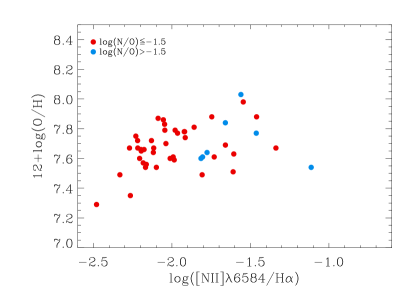
Figure 6.— Oxygen abundance versus N2 for the metal-poor galaxy sample. Red filled circles stand for galaxies log(N/O)$\leq$-1.5, whereas blue filled circles represent galaxies with log(N/O)$>$-1.5.

6. Summary and Final Remarks

Our initial aim was improving the calibration used in the literature to infer oxygen abundance from N2 for low-metallicity galaxies. In particular, we compare N2 and metallicity determined using the direct method in the set of XMP galaxies worked out by Morales-Luis et al. (2011). The first result is that the oxygen abundances obtained using the direct method confirm that galaxies classified as low-metallicity galaxies in Morales-Luis et al. (2011) are, indeed, metal-poor. The second result is more discouraging though. The observed oxygen abundance presents a tendency to be constant with N2 making it difficult to work out any calibration at low metallicity. Instead, we argue that the calibration O/H vs N2 by PP04 can be used at low metallicity to set an upper limit to the true metallicity (see Eq. 5).

O/H vs N2 presents a very large scatter (see Fig. 1). CLOUDY photoionization models allowed us to understand the scatter. We found that N2 decreases with the ionization parameter for a given oxygen abundance. Considering that the degree of ionization is related to the evolutionary state of the starburst ionizing the medium, we analyze the state of evolution using the equivalent width of H$\beta$. This analysis indicates that part of the dispersion observed is indeed due to the evolutionary state of the galaxies. In addition, we found that part of the scatter is also due to an excess of N/O in some of the metal-poor galaxies. An excess could be due to an extra production of primary nitrogen galaxies, or other processes including inflows of metal-poor gas (Sec. 5.2).

In short, we find the commonly used metallicity estimate based on N2 to be uncertain at low-metallicities. Fortunately, it is possible to use the N2 calibration to set an upper limit to the abundance in metal-poor galaxies.

References

- Aller (1984) Aller, L. H., ed. 1984, Astrophysics and Space Science Library, Vol. 112, Physics of thermal gaseous nebulae
- Alloin et al. (1979) Alloin, D., Collin-Souffrin, S., Joly, M., & Vigroux, L. 1979, A&A, 78, 200
- Amorín et al. (2012) Amorín, R., Pérez-Montero, E., Vílchez, J. M., & Papaderos, P. 2012, ApJ, 749, 185
- Amorín et al. (2010) Amorín, R. O., Pérez-Montero, E., & Vílchez, J. M. 2010, ApJ, 715, L128
- Andrews & Martini (2013) Andrews, B. H. & Martini, P. 2013, ApJ, 765, 140
- Asplund et al. (2009) Asplund, M., Grevesse, N., Sauval, A. J., & Scott, P. 2009, ARA&A, 47, 481
- Baldwin et al. (1981) Baldwin, J. A., Phillips, M. M., & Terlevich, R. 1981, PASP, 93, 5
- Berg et al. (2012) Berg, D. A., Skillman, E. D., Marble, A. R., et al. 2012, ApJ, 754, 98
- Castellanos et al. (2002) Castellanos, M., Díaz, A. I., & Terlevich, E. 2002, MNRAS, 337, 540
- Cresci et al. (2010) Cresci, G., Mannucci, F., Maiolino, R., et al. 2010, Nature, 467, 811
- De Robertis et al. (1987) De Robertis, M. M., Dufour, R. J., & Hunt, R. W. 1987, JRASC, 81, 195
- Denicoló et al. (2002) Denicoló, G., Terlevich, R., & Terlevich, E. 2002, MNRAS, 330, 69
- Edmunds & Pagel (1978) Edmunds, M. G. & Pagel, B. E. J. 1978, MNRAS, 185, 77P
- Erb (2008) Erb, D. K. 2008, ApJ, 674, 151
- Ferland et al. (1998) Ferland, G. J., Korista, K. T., Verner, D. A., et al. 1998, PASP, 110, 761
- Fisher et al. (2014) Fisher, D. B., Bolatto, A. D., Herrera-Camus, R., et al. 2014, Nature, 505, 186
- Gavilán et al. (2006) Gavilán, M., Mollá, M., & Buell, J. F. 2006, A&A, 450, 509
- Gonzalez-Delgado et al. (1994) Gonzalez-Delgado, R. M., Perez, E., Tenorio-Tagle, G., et al. 1994, ApJ, 437, 239
- Hägele et al. (2008) Hägele, G. F., Díaz, Á. I., Terlevich, E., et al. 2008, MNRAS, 383, 209
- Henry et al. (2000) Henry, R. B. C., Edmunds, M. G., & Köppen, J. 2000, ApJ, 541, 660
- Izotov et al. (2006) Izotov, Y. I., Stasińska, G., Meynet, G., Guseva, N. G., & Thuan, T. X. 2006, A&A, 448, 955
- James et al. (2013) James, B. L., Tsamis, Y. G., Barlow, M. J., Walsh, J. R., & Westmoquette, M. S. 2013, MNRAS, 428, 86
- Kehrig et al. (2013) Kehrig, C., Pérez-Montero, E., Vílchez, J. M., et al. 2013, MNRAS, 432, 2731
- Kewley et al. (2001) Kewley, L. J., Dopita, M. A., Sutherland, R. S., Heisler, C. A., & Trevena, J. 2001, ApJ, 556, 121
- Kniazev et al. (2004) Kniazev, A. Y., Pustilnik, S. A., Grebel, E. K., Lee, H., & Pramskij, A. G. 2004, ApJS, 153, 429
- Kunth & Östlin (2000) Kunth, D. & Östlin, G. 2000, A&A Rev., 10, 1
- Lagos et al. (2009) Lagos, P., Telles, E., Muñoz-Tuñón, C., et al. 2009, AJ, 137, 5068
- Leitherer et al. (1999) Leitherer, C., Schaerer, D., Goldader, J. D., et al. 1999, ApJS, 123, 3
- Levesque et al. (2010) Levesque, E. M., Kewley, L. J., & Larson, K. L. 2010, AJ, 139, 712
- López-Sánchez et al. (2012) López-Sánchez, Á. R., Koribalski, B. S., van Eymeren, J., et al. 2012, MNRAS, 419, 1051
- López-Sánchez et al. (2011) López-Sánchez, Á. R., Mesa-Delgado, A., López-Martín, L., & Esteban, C. 2011, MNRAS, 411, 2076
- Mannucci et al. (2011) Mannucci, F., Salvaterra, R., & Campisi, M. A. 2011, MNRAS, 414, 1263
- Marino et al. (2013) Marino, R. A., Rosales-Ortega, F. F., Sánchez, S. F., et al. 2013, A&A, 559, A114
- Miller & Mathews (1972) Miller, J. S. & Mathews, W. G. 1972, ApJ, 172, 593
- Mollá et al. (2006) Mollá, M., Vílchez, J. M., Gavilán, M., & Díaz, A. I. 2006, MNRAS, 372, 1069
- Monreal-Ibero et al. (2010) Monreal-Ibero, A., Vílchez, J. M., Walsh, J. R., & Muñoz-Tuñón, C. 2010, A&A, 517, A27
- Morales-Luis et al. (2011) Morales-Luis, A. B., Sánchez Almeida, J., Aguerri, J. A. L., & Muñoz-Tuñón, C. 2011, ApJ, 743, 77
- Nagao et al. (2006) Nagao, T., Maiolino, R., & Marconi, A. 2006, A&A, 459, 85
- Nicholls et al. (2014) Nicholls, D. C., Dopita, M. A., Sutherland, R. S., et al. 2014, ApJ, 786, 155
- Pagel et al. (1979) Pagel, B. E. J., Edmunds, M. G., Blackwell, D. E., Chun, M. S., & Smith, G. 1979, MNRAS, 189, 95
- Pagel et al. (1992) Pagel, B. E. J., Simonson, E. A., Terlevich, R. J., & Edmunds, M. G. 1992, MNRAS, 255, 325
- Peimbert & Peimbert (2010) Peimbert, A. & Peimbert, M. 2010, ApJ, 724, 791
- Pérez-Montero & Contini (2009) Pérez-Montero, E. & Contini, T. 2009, MNRAS, 398, 949
- Pérez-Montero & Díaz (2003) Pérez-Montero, E. & Díaz, A. I. 2003, MNRAS, 346, 105
- Pérez-Montero & Díaz (2005) Pérez-Montero, E. & Díaz, A. I. 2005, MNRAS, 361, 1063
- Pérez-Montero et al. (2010) Pérez-Montero, E., García-Benito, R., Hägele, G. F., & Díaz, Á. I. 2010, MNRAS, 404, 2037
- Pérez-Montero et al. (2013) Pérez-Montero, E., Kehrig, C., Brinchmann, J., et al. 2013, Advances in Astronomy, 2013
- Pérez-Montero et al. (2011) Pérez-Montero, E., Vílchez, J. M., Cedrés, B., et al. 2011, A&A, 532, A141
- Pettini & Pagel (2004) Pettini, M. & Pagel, B. E. J. 2004, MNRAS, 348, L59
- Queyrel et al. (2012) Queyrel, J., Contini, T., Kissler-Patig, M., et al. 2012, A&A, 539, A93
- Queyrel et al. (2009) Queyrel, J., Contini, T., Pérez-Montero, E., et al. 2009, A&A, 506, 681
- Sánchez Almeida et al. (2014) Sánchez Almeida, J., Morales-Luis, A. B., Muñoz-Tuñón, C., et al. 2014, ApJ, 783, 45
- Stasińska (2004) Stasińska, G. 2004, in Cosmochemistry. The melting pot of the elements, ed. C. Esteban, R. García López, A. Herrero, & F. Sánchez, 115–170
- Stasińska et al. (2012) Stasińska, G., Prantzos, N., Meynet, G., et al. 2012, in EAS Publications Series, Vol. 54, EAS Publications Series, ed. G. Stasińska, N. Prantzos, G. Meynet, S. Simón-Díaz, C. Chiappini, M. Dessauges-Zavadsky, C. Charbonnel, H.-G. Ludwig, C. Mendoza, N. Grevesse, M. Arnould, B. Barbuy, Y. Lebreton, A. Decourchelle, V. Hill, P. Ferrando, G. Hébrard, F. Durret, M. Katsuma, & C. J. Zeippen, 3–63
- Storchi-Bergmann et al. (1994) Storchi-Bergmann, T., Calzetti, D., & Kinney, A. L. 1994, ApJ, 429, 572
- Troncoso et al. (2014) Troncoso, P., Maiolino, R., Sommariva, V., et al. 2014, A&A, 563, A58
- van Zee & Haynes (2006) van Zee, L. & Haynes, M. P. 2006, ApJ, 636, 214