The Next Generation Virgo Cluster Survey. XV. The photometric redshift estimation for background sources

Abstract

The Next Generation Virgo Cluster Survey is an optical imaging survey covering 104 deg² centered on the Virgo cluster. Currently, the complete survey area has been observed in the $u^{*}giz$-bands and one third in the $r$-band. We present the photometric redshift estimation for the NGVS background sources. After a dedicated data reduction, we perform accurate photometry, with special attention to precise color measurements through point spread function-homogenization. We then estimate the photometric redshifts with the Le Phare and BPZ codes. We add a new prior which extends to $i_{AB}=12.5$ mag. When using the $u^{*}griz$-bands, our photometric redshifts for $15.5\leq i\lesssim 23$ mag or $z_{\rm phot}\lesssim 1$ galaxies have a bias $|\Delta z|<0.02$, less than 5% outliers, and a scatter $\sigma_{\rm outl.rej.}$ and an individual error on $z_{\rm phot}$ that increase with magnitude (from 0.02 to 0.05 and from 0.03 to 0.10, respectively). When using the $u^{*}giz$-bands over the same magnitude and redshift range, the lack of the $r$-band increases the uncertainties in the $0.3\lesssim z_{\rm phot}\lesssim 0.8$ range ($-0.05<\Delta z<-0.02$, $\sigma_{outl.rej}\sim 0.06$, 10-15% outliers, and $z_{\rm phot.err.}\sim 0.15$). We also present a joint analysis of the photometric redshift accuracy as a function of redshift and magnitude. We assess the quality of our photometric redshifts by comparison to spectroscopic samples and by verifying that the angular auto- and cross-correlation function $w(\theta)$ of the entire NGVS photometric redshift sample across redshift bins is in agreement with the expectations.

1. Introduction

Many fields of astronomy have entered a new era with the advent of large surveys (e.g., the Sloan Digital Sky Survey; SDSS; York et al. 2000), which give access to homogeneous observations for a large number of objects (up to $10^{6}$-$10^{8}$). Such large surveys provide invaluable information for studies of galaxy evolution and cosmology based on homogeneous measurements of a multitude of fundamental galaxy properties. In this context, a crucial quantity is the galaxy redshift.

While spectroscopic redshifts (spec-z’s) are unambiguous measurements, they are observationally too costly for $10^{6}$-$10^{8}$ objects. An alternative method, developed since the early ’60s (e.g., Baum 1962; Koo 1985), is the use of photometric redshifts (photo-z’s), which are estimated from photometry. Although less precise than spec-z’s, photo-z’s allow consistent measurement of redshifts for large numbers of galaxies, including relatively faint ones. The use of photo-z’s for large surveys is widespread today (e.g., Ilbert et al. 2006; Coupon et al. 2009; Ilbert et al. 2009; Bielby et al. 2012; Hildebrandt et al. 2012; Dahlen et al. 2013; Jouvel et al. 2014) and will be essential for future missions (e.g., such as Euclid; Laureijs et al. 2011).

Existing codes to estimate photo-z’s can be broadly classified in two categories: template fitting and empirical estimators. Template fitting codes (e.g., hyperz: Bolzonella et al. 2000; bpz – Bayesian photometric redshift: Benítez 2000; Le Phare – Photometric Analysis for Redshift Estimate: Arnouts et al. 1999, 2002; Ilbert et al. 2006; Eazy – Easy and Accurate Redshifts from Yale: Brammer et al. 2008) use empirical or theoretical galaxy spectra to find through fitting the redshift/template combination that best reproduces the observed colors, whereas empirical estimators (e.g., ANNz – Photometric redshifts using Artificial Neural Networks: Collister & Lahav 2004; Ball et al. 2008; ArborZ: Gerdes et al. 2010) use a representative sample to train machines like neural networks and reproduce the relation between the observed colors/magnitudes and the redshifts. The main limitations to estimate accurate photo-z’s are the wavelength coverage of key spectral features (e.g., the Lyman-break and the 4,000 Å/Balmer break), and the quality and homogeneity of the photometry. Hildebrandt et al. (2010) and Dahlen et al. (2013) have conducted thorough analyzes on the performance of the most popular algorithms. Both studies agree that the majority of the codes provides quantitatively similar results. Dahlen et al. (2013) find that the photo-z’s accuracy depends strongly on the magnitude.

We present in this paper the estimation of photo-z’s for the Next Generation Virgo Cluster Survey (NGVS; Ferrarese et al. 2012) with two template fitting codes: Le Phare and bpz. The NGVS is a comprehensive optical imaging survey of the Virgo cluster, from its core to its virial radius – covering a total area of 104 deg² – in the Canada-France-Hawaii Telescope (CFHT) $u^{*}griz$ bandpasses. The NGVS will serve as the optical reference survey over the Virgo cluster, and will leverage the numerous other surveys targeting Virgo at shorter and longer wavelengths, such as – to cite only the most recent ones: the Galaxy Evolution Explorer (GALEX) survey of Virgo in the ultra-violet (GUViCS; Boselli et al. 2011), the Next Generation Virgo Cluster Survey–Infrared in the near-infrared (NGVS-IR; Muñoz et al. 2014), the Herschel Virgo Cluster Survey in the far-infrared (HeViCS; Davies et al. 2010, 2012), or the Arecibo Legacy Fast ALFA Survey in the radio (ALFALFA; Giovanelli et al. 2005; Kent et al. 2008; Haynes et al. 2011).

The plan of this paper is as follows. Section 2 presents the data and their reduction. Section 3 details how we build the photometric catalogs. Section 4 presents the method to estimate the photo-z’s, Section 5 analyzes their quality, and Section 6 gives a science validation of our photo-z’s. We conclude in Section 7.

In this paper, we adopt $H_{0}=70$ km s^-1 Mpc^-1, $\Omega_{m}=0.30$, and $\Omega_{\Lambda}=0.70$. All magnitudes are in the AB system and corrected for the Galactic foreground extinction using the Schlegel et al. (1998) maps.

2. NGVSLenS data

In this paper, we use a NGVS dataset whose reduction is optimized for background-science (see below): we label this dataset NGVSLenS. We describe in this Section the data acquisition along with their reduction.

2.1. NGVSLenS data

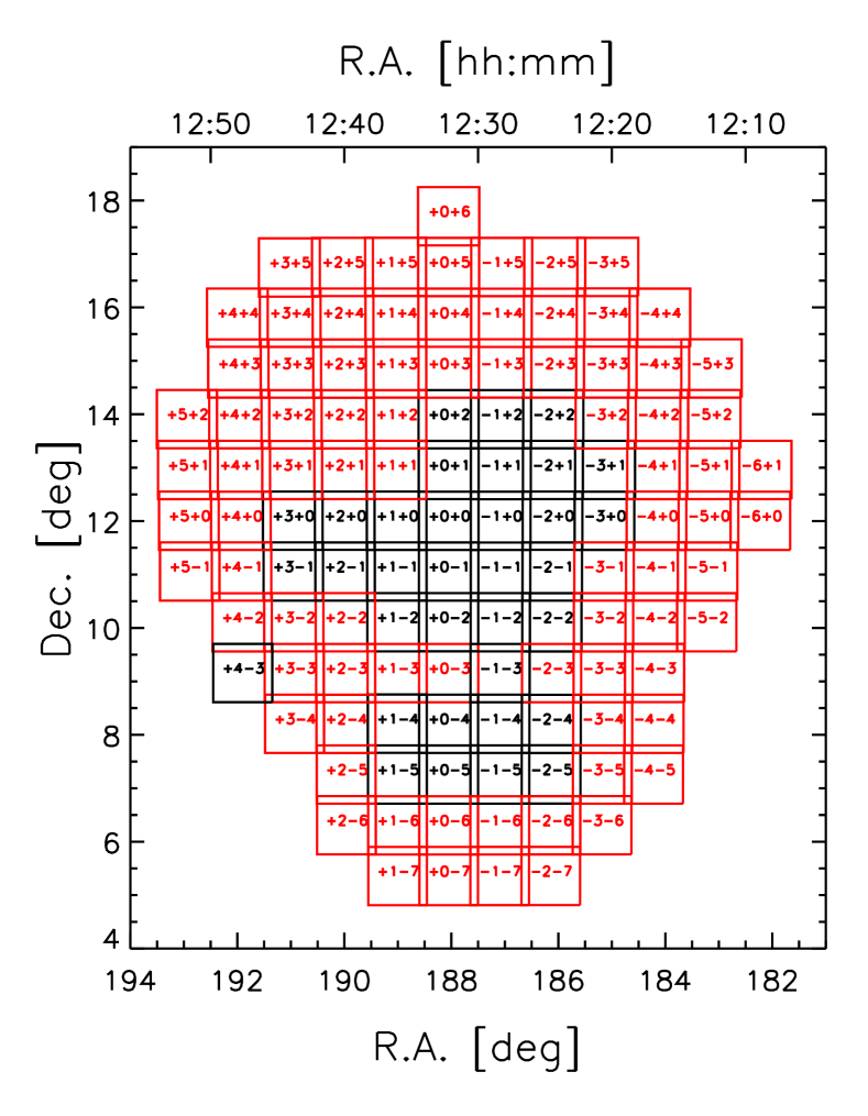
Figure 1.— Layout of the NGVS survey footprint. Pointings in black (red, respectively) have coverage in $u^{*}griz$ ($u^{*}giz$, respectively).

The imaging data used in this article are from the Next Generation Virgo Cluster Survey (NGVS; P.I. L. Ferrarese). The goals of the survey, its implementation and its observations have been described in detail in Ferrarese et al. (2012) and we only briefly repeat details relevant to this article.

The NGVS is a deep, 104 deg² multi-color optical imaging survey of the Virgo cluster. All the data are obtained with the MegaCam instrument (see Boulade et al. 2003) which is mounted on the CFHT. MegaCam is an optical multi-chip camera with a $9\times 4$ CCD array ($2048\times 4096$ pixels in each CCD; $0\hbox{$.\!\!^{\prime\prime}$}187$ pixel scale; $\sim$$1^{\circ}\times 1^{\circ}$ total field-of-view). NGVS observations were carried out with 117 discrete MegaCam pointings around the NGVS central position RA=12^h32^m12^s, Dec=12^d00^m19^s, that includes Virgo’s cD M87. The exact NGVS survey layout is shown in Figure 1. In this article, we follow the NGVS convention to label individual NGVS pointings (see Figure 4 of Ferrarese et al. 2012), which indicate the approximate separation in degrees from the NGVS central position. For instance, pointing “NGVS-1+2” is about one degree west and two degrees north of the NGVS center. We however caution that the data itself are processed with a slightly different convention (e.g., “NGVSm1p2” – read “NGVS minus 1 plus 2” – instead of “NGVS-1+2”).

The complete NGVS area (117 pointings) is covered in four SDSS-like filters: $u^{*}$ (CFHT identification: u.MP9301), $g$ (g.MP9401), $i$ (i.MP9702), and $z$ (z.MP9801). Additionally, 34 pointings also benefit from $r$ (r.MP9601) band coverage (see Figure 1).

Table 1 contains observational details and provides average quality characteristics of the final, co-added NGVS data used in this article. It lists average observing time for the different filters, the mean limiting magnitudes and the mean seeing values with their corresponding standard deviations over all 117 NGVS pointings. The seeing is estimated using the SExtractor (Bertin & Arnouts 1996) parameter FWHM_IMAGE for stellar sources. Our limiting magnitude, $m_{\rm lim}$, is the 5$\sigma$ detection limit in a $2\hbox{$.\!\!^{\prime\prime}$}0$ aperture. The complete NGVS data set was obtained under very good observing conditions. In Figure 2 we show the full seeing distribution for all fields and filters (see also Figure 8 of Ferrarese et al. 2012). We specifically note the superb seeing distribution of the $i$-band: the complete survey was obtained in this filter with an exceptional seeing of $<0\hbox{$.\!\!^{\prime\prime}$}6$.

Table 1Average characteristics of the NGVS co-added data used in this study (see the text for an explanation of the columns).

Filter	expos. time	$m_{\rm lim}^{\dagger}$	seeing
	[ks]	[AB mag]	[′′]
$u^{*}(u.MP9301)$	6.3	$25.60\pm 0.16$	$0.83\pm 0.07$
$g(g.MP9401)$	3.5	$25.73\pm 0.13$	$0.77\pm 0.08$
$r(r.MP9601)$	2.6	$24.68\pm 0.50^{\star}$	$0.74\pm 0.14$
$i(i.MP9702)$	2.3	$24.41\pm 0.13$	$0.52\pm 0.04$
$z(z.MP9801)$	4.6	$23.62\pm 0.16$	$0.70\pm 0.08$

Note. — ^†: $m_{\rm lim}$ is the 5$\sigma$ detection limit in a $2\hbox{$.\!\!^{\prime\prime}$}0$ aperture.

^⋆: for the $r$-band, the minimum and maximum values for $m_{\rm lim}$ are 23.56 and 25.52, respectively.

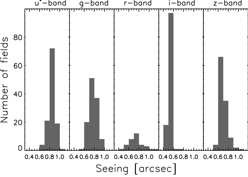
Figure 2.— Seeing distributions for all co-added NGVS fields and filters.

As detailed in Ferrarese et al. (2012), the NGVS data are used for a large variety of science projects. The different applications can be split in three categories: (1) the foreground-science, which will study the sources closer than the Virgo cluster; (2) the Virgo cluster itself; (3) and the background-science, which uses the deep data to study the higher redshift background galaxy populations. As outlined in Ferrarese et al. (2012), the NGVS team performs different data processing and produces a large variety of data products optimized for different science applications. Foreground- and Virgo science, requiring dedicated data processing, will be addressed in other publications by the NGVS collaboration (e.g., Durrell et al. 2014). The current study discusses the estimation of photo-z’s of background sources, which are crucial for the background-science. Future work will include the detection of high-redshift galaxy cluster candidates (Licitra et al., in preparation), and strong and weak lensing studies (e.g., Gavazzi et al., in preparation). Photo-z studies of faint background sources require high-quality, deep and carefully photometrically calibrated multi-color observations. In the following we provide information on the preparation of the necessary data products.

2.2. NGVSLenS data reduction

To process the NGVS data for background-science applications, we use the algorithms and processing pipelines (theli) developed within the CFHTLS-Archive Research Survey (CARS; see Erben et al. 2009) and the Canada-France-Hawaii-Telescope Lensing Survey (CFHTLenS; see Heymans et al. 2012; Hildebrandt et al. 2012; Erben et al. 2013, and http://cfhtlens.org). Both surveys originated from the Wide component of the Canada-France-Hawaii-Telescope Legacy Survey (CFHTLS; Gwyn 2012) which was also obtained with MegaCam. In addition, the survey characteristics and the observing strategies of CFHTLS and NGVS are very similar. This allowed for a direct transfer of our CFHTLS expertise to NGVS. In the following we only give a very short description of our procedures to arrive at the final co-added images for NGVS. All algorithms and prescriptions are described in detail in Erben et al. (2013). The interested reader should consult this article and the references therein. Below, we also give a more detailed analysis of the quality from our photometric calibration which is crucial for the quality of photometric redshift estimates.

Our NGVS data processing consisted of the following steps:

1. Data sample:
   We start our data analysis with the Elixir preprocessed NGVS data available at the Canadian Astronomical Data Centre (CADC). For the current study we used NGVS observations obtained from 01/03/2008 until 12/06/2013. The data were obtained under several CFHT programs (P.I. L. Ferrarese: 08AC16, 09AP03, 09AP04, 09BP03, 09BP04, 10AP03, 10BP03, 11AP03, 11BP03, 12AP03, 12BP03, 13AC02, 13AP03; P.I. Simona Mei: 08AF20; P.I. Jean-Charles Cuillandre: 10AD99, 12AD99 and P.I. Ying-Tung Chen: 10AT06). From the initial set we reject all short exposed NGVS images. To be able to study bright cores of Virgo galaxies, the NGVS obtained, besides the primary science data, numerous short exposures in all pointings and filters (see Section 3.4 of Ferrarese et al. 2012). Because these exposures would not contribute an appreciable fraction to the total exposure time in each filter, we did not consider them further. We also do not use images whose observing conditions were marked as unfavourable by CFHT.

2. Single exposure processing:
   The Elixir preprocessing includes a complete removal of the instrumental signature from raw data (see also Magnier & Cuillandre 2004). In addition, each exposure comes with all necessary photometric calibration information. Therefore, we only need to perform the following processing steps on single exposures: (1) we identify and mark individual exposure chips that should not be considered any further. This mainly concerns chips which are completely dominated by saturated pixels from a bright star. (2) We create sky-subtracted versions of the images. In the context of NGVS we create a so-called local sky-background subtraction optimal for the study of faint background galaxies (see also Figure 11 of Ferrarese et al. 2012). In addition, we create a weight image for each science chip. It gives information on the relative noise properties of individual pixels and assigns a weight of zero to defective pixels (such as cosmic rays, hot and cold pixels, areas of satellite tracks). (3) We use SExtractor to extract high $S/N$ sources from the science image and weight information. These source catalogs are used to astrometrically and photometrically calibrate the data in the next processing step. In addition we perform an analysis of the PSF anisotropy and use this information to reject images showing high stellar ellipticities. Highly elongated point sources are a good indication of tracking issues or other severe problems during an exposure.

3. Astrometric and Photometric calibration:
   We use the scamp software (see Bertin 2006) to astrometrically calibrate the NGVS survey. We use the Two Micron All Sky Survey (2MASS; Skrutskie et al. 2006) as astrometric reference and calibrate separately each filter from the NGVS patch (i.e., all fields) with scamp. Once an astrometric solution is established we use overlap sources from individual exposures to establish an internal, relative photometric solution for all exposures. We reject all exposures with an absorption of more than 0.2 magnitudes and rerun scamp on the remaining images. With the relative photometric solution and the Elixir zeropoint information we estimate a patch-wide photometric zeropoint for each filter.

4. Image co-addition and mask creation:
   The next step of our image processing co-adds the sky-subtracted exposures belonging to a pointing/filter combination with the swarp program (see Bertin et al. 2002). The stacking is performed with a statistically optimally weighted mean which takes into account sky-background noise, weight maps and the scamp relative photometric zeropoint information. As a final step we use the automask tool (see Dietrich et al. 2007) to create image masks for all pointings. These masks flag bright, saturated stars and areas which would influence the analysis of faint background sources. For the NGVS, a reliable masking of bright Virgo members is particularly important for our purposes. The 117 generated masks have been visually checked (A.R.). In a typical NGVS pointing we loose about 20%-30% of the area because of masking, as can be seen in Figure 3, where we display those masks for a section of a field. In the figure we note that several algorithms and template masks are used to mask different artifacts, e.g., bright stars, short asteroid trails or large-scale bright objects. The artifacts we consider and the way we treat them is described in more detail in Erben et al. (2009).

5. Photometric calibration tied to the SDSS:
   The final step is specific to the NGVS, i.e., it has not been implemented in the released CFHTLenS. Taking advantage of accurate internal photometric stability of the SDSS, and of its full coverage of the NGVS field, we tie our photometric calibration to the SDSS. We retrieve clean stars from the SDSS-DR10 (Ahn et al. 2014) and convert their Petrosian magnitude to the MegaCam photometric system using Equation (4) of Ferrarese et al. (2012). For each field and each filter available, we then measure the MAG_AUTO with SExtractor and correct for the offset between the two catalogs by taking the median value for a subset of bright non-saturated stars ($\sim$500 per field). The typical uncertainty in this calibration step is of 0.05 mag in the $griz$-bands and of 0.10 mag in the $u$-band. We note that the theli photometry is homogeneous over the NGVS field, with a field-to-field standard deviation of $\sim$0.03 mag, as found in Erben et al. (2013).

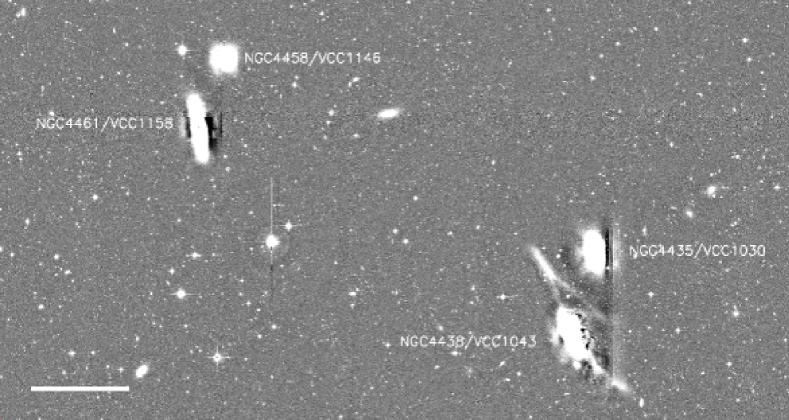
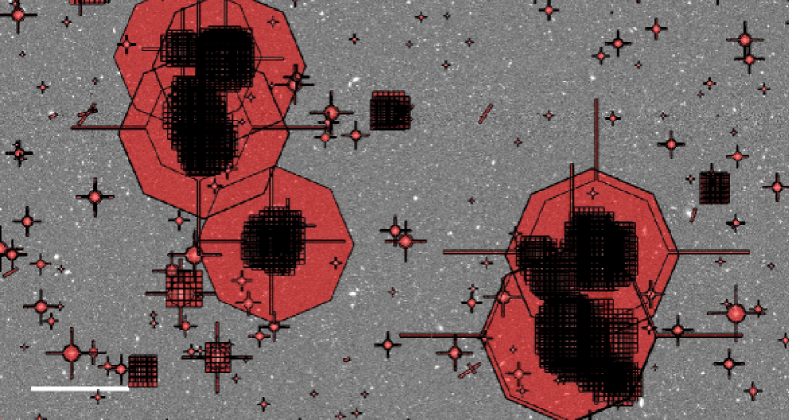
Figure 3.— Image mask of a $40\hbox{$.\!\!^{\prime}$}\times 25\hbox{$.\!\!^{\prime}$}$ section of the NGVS-1+1 pointing. Our automatic masking reliably picks up bright stars and Virgo galaxies that would influence photometric analyzes of faint background galaxies through their light halos (which are an artifact of the local background subtraction). Different mask shapes correspond to different artifacts (see text). We identify the prominent Virgo galaxies in this field. The ruler (white bar on the bottom-left side) is $5\hbox{$.\!\!^{\prime}$}$ wide.

3. Photometric catalogs

For simplicity, we hereafter are referring to NGVSLenS when referring to NGVS or the NGVSLenS dataset, and similarly to CFHTLenS with CFHTLS or the CFHTLenS dataset.

In this Section we describe the procedure to build the photometric catalogs when the five $u^{*}griz$-bands are available (the procedure is similar when only the four $u^{*}giz$-bands are available). As studied in detailed in Hildebrandt et al. (2012), a requirement to estimate precise photo-z’s is accurate photometry, in particular high precision color measurements. To do so, we implement the following procedure (global mode of Hildebrandt et al. 2012): the $i$-band, which has the best seeing ($0.52\arcsec\pm 0.04\arcsec$), is used to detect objects and estimate their total magnitude; then, for each field, all images are first homogenized to the same PSF and then used to estimate accurate colors.

3.1. Global PSF homogenization

The photometric catalogs are constructed as described in Hildebrandt et al. (2012), which also describe the global PSF homogenization that is necessary to measure unbiased colors. According to the Hildebrandt et al. (2012) analysis, done on the CFHTLenS data having properties similar to the NGVSLenS data ones (see Section 5 and Appendix B), the quality of the photo-z’s obtained assuming a constant PSF across each field (global mode) provides satisfactory results, even when compared to that obtained when accounting for the PSF variations across each field (local mode). For this analysis, we hence consider that it is satisfactory to make the approximation that the PSF is constant over each field (1 deg²) and can be described by a single Gaussian with width $\sigma_{\rm PSF}$.

For each field, we identify the band which has the largest seeing ($\sigma_{\rm PSF,worst}$) and we bring the other four images to the same seeing by convolving them with a two-dimensional Gaussian filter. For instance if the $X$-band image has a PSF width $\sigma_{\rm PSF,X}$, we convolve it with a Gaussian filter of width $\sqrt{\sigma_{\rm PSF,worst}^{2}-\sigma_{\textrm{PSF},X}^{2}}$. The 117 values values of $\sigma_{\rm PSF,worst}$ have a mean value of $0.85\pm 0.07$, and the band with $\sigma_{\rm PSF,worst}$ is the $u^{*}$- ($g$-, $r$-, $i$-, and $z$-, respectively) band in 58 (45, 7, 0, and 7, respectively) fields.

3.2. Photometry method

Multicolor catalogs in the $u^{*}griz$ bands are extracted from a set of these PSF homogenized images using SExtractor in dual-image mode, using the un-convolved $i$-band image as the detection image. One SExtractor run is performed on the un-convolved $i$-band image for detection, structural measurements, and estimation of the total $i$-band magnitudes (SExtractor MAG_AUTO). Five SExtractor runs (dual-image mode, with the un-convolved $i$-band image as the detection image) are then performed with the PSF-matched $u^{*}griz$ images to measure accurate colors. Indeed, the obtained isophotal magnitudes MAG_ISO are measured on the same physical apertures, as we are using the same pixels (dual-mode) of PSF-matched images. From this procedure, we obtain accurate measurements for the colors and the $i$-band total magnitude; estimation of the total magnitude in the $u^{*}grz$ bands can be obtained with (Hildebrandt et al. 2012):

$$X_{\rm tot}=i_{\rm tot}+(X-i),\;\textnormal{with}\;X\in\{u^{*},g,r,z\},$$ (1)

where $X_{\rm tot}$ and $i_{\rm tot}$ are the total magnitudes in the $X$ and $i$ bands respectively, and $(X-i)$ is the corresponding color index. Note that we do not use the estimations of the total magnitude in the $u^{*}grz$ bands. Also, we caution that these estimations will only be valid if the galaxies do not present strong color gradients.

3.3. Photometric errors

In this study, we pay special attention to the photometric error estimation. Noise correlation introduced by image resampling during the reduction artificially decreases the pixel-to-pixel rms variations $\sigma_{1}$, which leads to an underestimation of the flux errors estimated by SExtractor (e.g. Casertano et al. 2000). This effect is known and the flux error underestimation factor for the CFHT/MegaCam optical bands is of the order of 1.5 (e.g., Ilbert et al. 2006; Coupon et al. 2009; Raichoor & Andreon 2012). However, it can be much larger on convolved images and the flux error underestimation factor can be of the order of 5, as shown by our data analysis (see Figure 4). This phenomenon can be more pronounced in the presence of fringing (Ferrarese et al. 2012). We choose the following method to estimate the true background fluctuations, $\sigma_{\rm bkg}$: regardless of whether the measurement is performed on a convolved or un-convolved image, we estimate $\sigma_{\rm bkg}$ in the un-convolved image, as it is not affected by the convolution process.

For each of our 502 un-convolved images, we estimate $\sigma_{\rm bkg}$ by placing 2,000 random apertures of a given size, which do not overlap with any detected objects (e.g. Labbé et al. 2003; Gawiser et al. 2006). We use circular apertures of area $n_{\rm pix}$ centered at integer pixels and describe them by the linear size of the aperture defined as $N=\sqrt{n_{\rm pix}}$, and fit a Gaussian to the histogram of aperture fluxes to yield $\sigma_{\rm bkg}(N)$, the background fluctuation for a given aperture $N$. We apply this method for $0\arcsec<N<3\arcsec$. Then we fit the obtained $\sigma_{\rm bkg}(N)$ curve as a function of $N$ following Labbé et al. (2003) formalism:

$$\sigma_{\rm bkg}(N)=\sigma_{1}\times(aN+bN^{2}).$$ (2)

$\sigma_{1}=\sigma(1)$ is the pixel-to-pixel rms variations, measured through 1 pixel apertures for each un-convolved image for a given band and a given field. We present in Table 2 the median of the 502 fitted values for $\sigma_{1}$, $a$, and $b$.

Table 2Median values of the image noise parameters fitted with Eq.(2).

Filter	$\sigma_{1}$	$a$	$b$
	[count.s-1]
$u$	$0.008\pm 0.001$	$0.995\pm 0.037$	$0.046\pm 0.005$
$g$	$0.020\pm 0.002$	$1.029\pm 0.038$	$0.046\pm 0.007$
$r$	$0.036\pm 0.022$	$1.054\pm 0.047$	$0.041\pm 0.012$
$y$	$0.040\pm 0.005$	$1.025\pm 0.039$	$0.044\pm 0.007$
$z$	$0.030\pm 0.004$	$0.865\pm 0.059$	$0.110\pm 0.028$

Using error propagation and Poissonian uncertainties, the magnitude uncertainty $\Delta m$ for an object with a measured flux $F$ (in ADU.s^-1) and a pixel area $n_{\rm pix}$ is obtained by accounting for the background noise and the Poissonian noise intrinsic to the object:

$$\Delta m=\frac{2.5}{ln10}\times\frac{1}{w}\times\frac{\sqrt{F/g+[\sigma_{\rm bkg}(\sqrt{n_{\rm pix}})]^{2}}}{F},$$ (3)

where $g$ is the gain and $w$ is the square root of the number of single frames that contribute to the considered pixels divided by the number of single frames used to build the un-convolved image (which gives an estimation of the weight on the considered pixels; cf. Erben et al. 2013). We use the SExtractor outputs for the flux $F$ and the pixel area $n_{\rm pix}$ estimations.

We illustrate in Figure 4 how our estimated photometric uncertainties compare with those of SExtractor for the NGVS+0+0 field. When the images are not convolved ($z$-band for this field), we recover the usual SExtractor underestimation of $\sim$1.5 because of pixel correlation. However, we see that the underestimation is much greater when SExtractor is run on a convolved image, and that this underestimation is a function of the convolution kernel and of the object’s magnitude (and size). When plotting the individual objects (bottom panels), we remark that stars have a different behavior, because of their small $n_{\rm pix}$, compared to galaxies of similar magnitude.

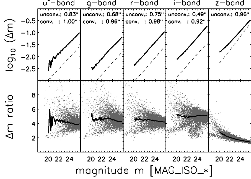
Figure 4.— Re-estimated magnitude error ($\Delta m$) properties for the NGVS+0+0 field. The continuous and dashed lines show the median values for $20\leq m\leq 26$ mag. Top panel: we show $\Delta m$ as a function of magnitude $m$; our re-estimated errors are shown as continuous lines while SExtractor errors are denoted by dashed lines. We report for each band the seeing before and after convolution (for the NGVS+0+0 field, the $z$-band image is the one with the worst seeing, hence it is not convolved). Bottom panel: we show the ratio of our $\Delta m$ to SExtractor’s $\Delta m$ as a function of magnitude $m$; points illustrate the individual distribution of objects (for clarity, we plot only 1 out of 5 points). SExtractor errors are on average underestimated by a factor of $\sim$4-5 on convolved images and of $\sim$2 on un-convolved images.

4. Photometric redshifts estimation

With the photometric catalogs described in the previous section in hand, we are able to estimate the photo-z’s. We describe in this section the procedure used to estimate them. In Table 3, we summarize the setup parameters used in this analysis.

Table 3Photo-z setup parameters summary.

Parameter	Comment
Template set	El, Sbc, Scd, Im, SB2, SB3 (Capak et al. 2004)
Prior	Appendix A (Le Phare prior for $i>20$ mag, extended down to $i=12.5$ mag)
$E(B-V)$ reddening	Le Phare: $0\leq E(B-V)\leq 0.25$; BPZ: none
Reddening law	Le Phare: Prevot et al. (1984); BPZ: none
Minimum photometric error	$rgiz$-band: 0.05 mag; $u$-band: 0.10 mag

4.1. Code: Le Phare and BPZ

In the present study, we use two template-based codes to estimate photo-z’s: Le Phare (Arnouts et al. 1999, 2002; Ilbert et al. 2006) and bpz (Benítez 2000; Benítez et al. 2004; Coe et al. 2006). In addition to having been widely used and tested, Hildebrandt et al. (2010) and Dahlen et al. (2013) have shown that these two codes provide satisfactory results.

4.2. Templates

For both codes, we use the recalibrated template set of Capak et al. (2004), which is built from the four Coleman et al. (1980) observed galaxy spectra (El, Sbc, Scd, Im), with two additional observed starburst templates from Kinney et al. (1996). We note that, when running Le Phare and bpz, those six templates are linearly interpolated into $\sim$60 templates, so to have a better sampling of the color space.

A requirement of our template set is its ability to reproduce the observed colors. In Figure 5, we display the observed colors for our spectroscopic sample ($\sim$83,000 galaxies; described in Section 5.1), along with the colors predicted by the templates. Our templates cover in a satisfactory way the observed colors. We note that galaxies having a $u-r$ color redder than the models are a minority: for instance, less than 3% of galaxies with $0.4<z_{\rm spec}<0.9$ have $u-r>5$ mag.

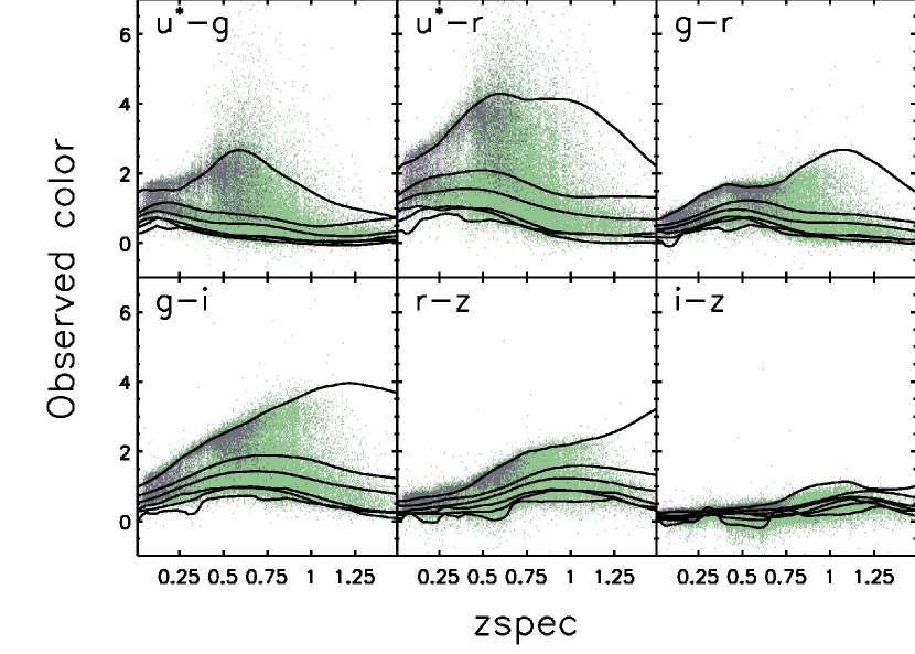
Figure 5.— Observed colors as a function of $z_{\rm spec}$: magenta and green dots show our NGVSLenS and CFHTLenS spectroscopic samples, respectively (both described in Section5.1); black lines represent the colors predicted by our adopted template set. Our template set satisfactorily reproduces the observed colors.

Le Phare offers the possibility to include galaxy internal reddening, $E(B-V)$ as a free parameter during the fit. When running Le Phare for spectral types later than Sbc, we let $E(B-V)$ as a free parameter ($0\leq E(B-V)\leq 0.25$) using the Small Magellanic Cloud (SMC) extinction law (Prevot et al. 1984) (see Coupon et al. 2009). We have tested that our results of Section 5 are independent of the use of an other extinction law (Large Magellanic Cloud (LMC), Fitzpatrick 1986) or a larger range of possible reddening ($0\leq E(B-V)\leq 0.5$).

4.3. Fitting procedure and new prior

Overall, both codes run in a similar way using a Bayesian approach. This approach, and more precisely the use of a prior, allows the estimate of robust photo-z’s; its advantage over the maximum-likelihood method is described in detail in Benítez (2000). Briefly, in the maximum-likelihood method, a priori assumptions are implicitly made on the choice of the explored parameter space. The Bayesian approach, with the use of a prior, implements a priori knowledge in a more systematic and detailed way. Regarding the photo-z estimation, thanks to the existence of large, intensive spectroscopic surveys coupled with imaging (e.g., SDSS; zCOSMOS: Lilly et al. 2007; DEEP2: Cooper et al. 2008; VVDS: Le Fèvre et al. 2013) we have some precise and statistically robust knowledge about the relationship between spec-z, magnitude, and spectral type. This a priori knowledge is used to favor more physical solutions and brings essential constraints when there are few bandpasses to estimate the photo-z’s, as it is the case in our work.

We now succinctly present the Bayesian approach (please refer to Benítez 2000, for a detailed presentation). For a given galaxy with an observed magnitude $m_{0}$ in a reference band ($i$-band here) and observed colors $C$, the posterior $p(z|m_{0},C)$, i.e., the probability for this galaxy to be at redshift $z$ given the observed data, can be expressed as a sum of probabilities over the basis formed by the different spectral distribution types, $T$, belonging to our template set (see Section 4.2 and Table 3):

$$p(z|m_{0},C)=\sum_{T}p(z,T|m_{0},C),$$ (4)

where $p(z,T|m_{0},C)$ is the probability of the galaxy redshift being $z$ and the galaxy spectral template type being $T$. According to Bayes’ theorem, $p(z,T|m_{0},C)$ is proportional to the product of the likelihood $p(C|T,z)$ of observing those colors for a galaxy of spectral template type $T$ at redshift $z$ and of the prior $p(z,T|m_{0})$, which translates the a priori probability for a galaxy of magnitude $m_{0}$ to be at redshift $z$ and have a spectral template type $T$:

$$p(z,T|m_{0},C)\propto p(C|T,z)\times p(z,T|m_{0}).$$ (5)

To account for zeropoint uncertainty (see Section 2.2), we add in quadrature an uncertainty of 0.05 mag in the $griz$-bands and of 0.10 mag in the $u$-band. Those account for the typical uncertainties in our photometric calibration explained in Section 2.2. Both codes provide the redshift posterior distribution. We take as the photo-z estimate the median of this posterior distribution. We choose to use the median of the p(z) because it improves the redshift estimation in the most difficult cases in which the algorithm cannot define a clear peak of the distribution (see also the Dahlen et al. 2013 analysis when comparing results from different photo-z algorithms). This corresponds to the Z_ML output of Le Phare; bpz does not provide this output: we compute it based on the output posterior. Regarding the photo-z uncertainties, we use the boundary of the interval including 68% of the redshift probability distribution function. Le Phare outputs those as Z_ML68_LOW and Z_ML68_HIGH; bpz provides only 95% uncertainty on $z_{\rm phot}$: for each object, we compute, based on the output posterior, the 68% confidence interval as defined in Le Phare.

4.3.1 Introduction of a new prior

Le Phare and bpz were designed for high redshift studies: both codes use similar priors for $i>20$ mag galaxies, built with observed data. However, the priors used for $i<20$ mag galaxies are not calibrated on observed data and, as a consequence, do not provide satisfying constraints. A direct outcome is low-quality photo-z’s for $z_{\rm spec}\lesssim 0.2$ objects, for which the photo-z’s have either a large scatter with Le Phare (e.g., see Figure 11 of the CFHTLS/Wide T0007 paper) or are biased towards high values with bpz (e.g., see Figure 4 of Erben et al. 2009). As a result of the large area covered by the NGVSLenS, $i<20$ mag galaxies represent a non-negligible fraction of our sample: Hildebrandt et al. (2012) already noticed this issue with the CFHTLenS data – the bpz prior biasing the posterior against low photo-z’s – and implemented an ad hoc solution. We tackle this issue in a more systematic way by extending the prior to bright objects. We use the SDSS Galaxy Main Sample spectroscopic survey (York et al. 2000; Strauss et al. 2002; Ahn et al. 2014) to establish the prior for $13<i\leq 17$ mag galaxies, and extrapolate the prior for $17<i<20$ mag galaxies. The construction of this extended prior is detailed in Appendix A.

4.3.2 No photometric re-calibration

When using the template fitting method, it is common to add some photometric offsets during the fitting (e.g., Brodwin et al. 2006; Ilbert et al. 2006; Hildebrandt et al. 2010; Dahlen et al. 2013) because they can improve the accuracy of the estimated photo-z’s. They may correct for various effects, such as imprecise photometric calibration, mismatch between the used templates and spectral energy distributions of observed galaxies, imprecise filter throughputs, or different properties of source images when using multi-color catalogs. These offsets are calculated with an iterative process comparing the colors predicted from the templates with the colors measured for a spectroscopic subsample.

We have tested the computation of such offsets (using the bright objects of our spectroscopic sample described in Section 5.1). We find small offsets ($<0.03$ mag in absolute value) and hence do not use them in the present study. Our approach is in agreement with the analysis of Hildebrandt et al. (2012), who concluded that using PSF-matched photometry decreases the offset amplitude.

5. Photometric redshift accuracy

We present in this Section an analysis of our photo-z’s to quantify their accuracy.

As detailed below, our spectroscopic sample over the NGVSLenS field is rather shallow ($z\lesssim 0.8$) and highly biased at $z\gtrsim 0.3$. In order to assess the quality of our photometric redshifts up to $z<1.5$, we use the CFHTLenS data, which are covered by deep and intensive spectroscopic surveys.

Those CFHTLenS data have been imaged with the same telescope, instrument, filters (except for the $i$-band filter which was replaced), have similar depth, and have been reduced with the same theli pipeline. Starting from the CFHTLenS theli coadded-images, we re-estimate for the CFHTLenS the photometry and photo-z’s, with the theli pipeline including our modifications described in the previous sections (including the photometric calibration tied to the SDSS; see (v) of Section 2.2). We confirm a posteriori the close similarity of the CFHTLenS and NGVSLenS datasets in Appendix B.

We can thus compare our photo-z’s with two complementary spectroscopic samples, over the NGVSLenS and the CFHTLenS fields, as described in the next section.

In this analysis, we exclude very low redshift ($z\leq 0.01$) objects, mainly Virgo objects, as those are either spectroscopically confirmed (Virgo galaxies) or have redshifts difficult to constrain with optical data only (Virgo globular clusters – GCs – and Ultra-compact dwarf galaxies – UCDs). Muñoz et al. (2014) show that near-infrared data are crucial to diagnose those populations. Those objects, along with Galactic stars, are excluded either using the spec-z for the spectroscopic samples, either using the criteria presented in Appendix C for the photometric samples. We remark that our pipeline computes a photo-z for those objects, but we do not analyze it here.

In Section 5.1, we present the samples that we use to analyze our photo-z’s. We quantify, as a function of magnitude or redshift, the accuracy of our photo-z’s when they are estimated with the $u^{*}griz$-bands (Sections 5.2 and 5.3) or with the $u^{*}giz$-bands (Section 5.4). Section 5.5 presents a joint analysis of photo-z dependence on magnitude and redshift.

5.1. Samples definition

In this section, we present and define the samples used to analyze the accuracy of our photo-z’s. We first present the two spectroscopic samples covering the NGVSLenS and the CFHTLenS. We then present the photometric samples covering the NGVSLenS. The properties of those samples are summarized in Table 5.1.

Table 4Properties of the samples used in Section 5.

Survey	Number of galaxies	Area	Band coverage	$\langle z_{\rm spec}\rangle^{\dagger}$	$\langle i\rangle^{\dagger}$	Reference
	[$10^{3}$]	[deg2]			[mag]
Spectroscopic sample over the NGVSLenS field ($0.01\leq z_{\rm spec}<1.5$)
SDSS/GalMS	9.2	104	$u^{*}griz/u^{*}giz$	$0.11\pm 0.05$	$16.8\pm 1.1$	(1)
SDSS/notGalMS	14.3	104	$u^{*}griz/u^{*}giz$	$0.48\pm 0.13$	$19.3\pm 0.8$	(2)
AAT	1.4	$\sim$30	$u^{*}griz/u^{*}giz$	$0.15\pm 0.09$	$18.2\pm 0.6$	(3)
MMT	1.1	$\sim$4	$u^{*}griz$	$0.19\pm 0.10$	$18.7\pm 0.8$	(4)
Keck	0.1	-	$u^{*}griz/u^{*}giz$	$0.72\pm 0.37$	$23.2\pm 1.2$	(5)
Compiled	26.1	104	$u^{*}griz/u^{*}giz$	0.32$\pm$0.21	18.3$\pm$1.5	-
Spectroscopic sample over the CFHTLenS field ($0.01\leq z_{\rm spec}<1.5$)
SDSS/GalMS	0.8	$\sim$24	$u^{*}griz$	$0.11\pm 0.05$	$16.6\pm 0.6$	(1)
SDSS/notGalMS	5.6	$\sim$42	$u^{*}griz$	$0.41\pm 0.21$	$19.0\pm 1.6$	(2)
VVDS/F22	4.0	$\sim$3	$u^{*}griz$	$0.52\pm 0.23$	$21.4\pm 0.9$	(6)
VVDS/F02	5.0	$<1$	$u^{*}griz$	$0.69\pm 0.30$	$22.7\pm 1.2$	(6)
DEEP2/EGS	12.1	$<1$	$u^{*}griz$	$0.71\pm 0.32$	$22.5\pm 1.2$	(7)
VIPERS	29.6	$\sim$17	$u^{*}griz$	$0.68\pm 0.16$	$21.7\pm 0.8$	(8)
Compiled	57.2	42	$u^{*}griz$	0.65$\pm$0.25	21.6$\pm$1.5	-
Photometric samples over the NGVSLenS field
NGVSLenS/phot23	576.7	$\sim$30	$u^{*}griz$	-	$21.9\pm 1.0$	This paper
NGVSLenS/phot24	1,263.5	$\sim$30	$u^{*}griz$	-	$22.8\pm 1.1$	This paper

Note. — ^†: mean and standard deviation.

References. — (1): Strauss et al. (2002); (2): Eisenstein et al. (2001); Dawson et al. (2013); (3): Zhang et al. (submitted); Zhang et al. (in preparation); (4): Peng et al. (in preparation); (5): Guhathakurta et al. (in preparation); (6): Le Fèvre et al. (2005, 2013) (7): Davis et al. (2003); Newman et al. (2013) (8): Guzzo et al. (2013).

5.1.1 Spectroscopic sample over the NGVSLenS

The NGVSLenS field is covered by several spectroscopic surveys having different target selections. The entire NGVSLenS field is covered by the SDSS, providing $\sim$23,500 galaxy spec-z’s: $\sim$40% come from the Galaxy Main Sample, which is magnitude limited ($r\leq 17.77$; Strauss et al. 2002) and have $\langle z_{\rm spec}\rangle=0.11\pm 0.05$; the remaining $\sim$60% come from different target selection functions, mainly targeting luminous red galaxies (LRGs; Eisenstein et al. 2001; Dawson et al. 2013), have $\langle z_{\rm spec}\rangle=0.48\pm 0.13$, and represent by selection the most luminous galaxies at each redshift (e.g., see Figure 5 and bottom panel of Figure 6).

Other spectroscopic programs targeting candidate globular clusters or UCDs (MMT, P.I. E. Peng; Peng et al., in preparation; AAT, P.I.: P. Côté: Zhang et al., submitted; Zhang et al., in preparation) provide us with $\sim$2,500 spec-z’s ($\langle z_{\rm spec}\rangle=0.16\pm 0.12$). We also gathered $\sim$90 spec-z’s from the Virgo Dwarf Globular Cluster Survey taken with the Keck telescope (Keck, P.I.: P. Guhathakurta: Guhathakurta et al., in preparation): those are faint ($i=23.2\pm 1.2$ mag) emission lines galaxies that were either purposely targeted (e.g., missclassified as GC, dwarf elliptical) or are serendipitous sources that happened to land on the ”blank sky” portions of the slits. Because of its faintness, this subsample is very different from the rest of our NGVSLenS spectroscopic subsamples and provides a unique opportunity to probe – even sparsely – our photo-z’s up to $z_{\rm spec}\sim 1.5.$ for $21<i<24.5$ mag.

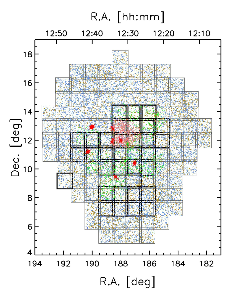
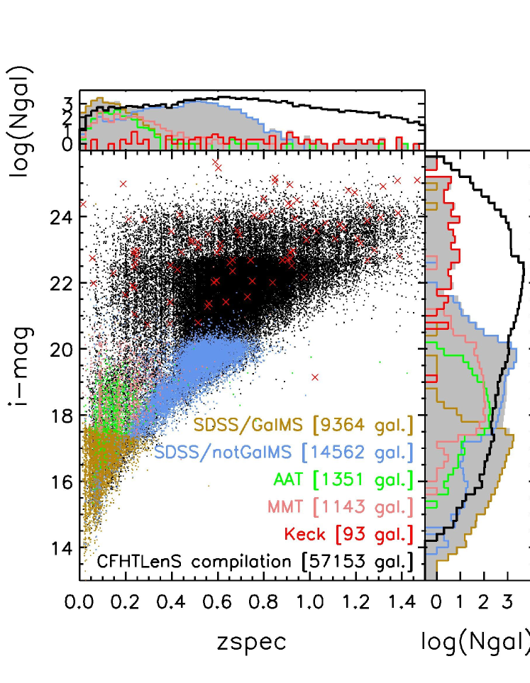
Figure 6.— Spectroscopic samples properties. Spec-z’s from the SDSS/Galaxy Main Sample (SDSS/other programs, AAT, MMT, Keck, respectively) survey are in gold points (blue points, green points, coral points, red crosses, respectively) symbols. The black points are the CFHTLenS spectroscopic sample (SDSS; VVDS F02/F22; DEEP2/EGS; VIPERS W1/W4). Left panel: we show the spatial distribution of the NGVSLenS spectroscopic sample; the fields covered by the $u^{*}griz$ bands have thick black outlines. Right panel: we show $i$-band magnitude as a function of $z_{\rm spec}$; the filled grey histograms represent the whole NGVSLenS spectroscopic sample.

We display in Figure 6 the spatial distribution (top panel) and $i$-band magnitude vs. $z_{\rm spec}$ distribution (bottom panel) of our spec-z compilation. Our spec-z compilation over the NGVSLenS is very heterogeneous and rather shallow in redshift ($\sim$50% with $z_{\rm spec}\lesssim 0.3$). At low redshift ($z_{\rm spec}\lesssim 0.3$), it covers a wide range of colors and galaxy types; however at higher redshifts ($z_{\rm spec}\gtrsim 0.3$), it is severely biased towards LRGs.

5.1.2 Spectroscopic sample over the CFHTLenS

To complement this spectroscopic sample, we use the public CFHTLenS data (Erben et al. 2013) covering three intensive and deep spectroscopic surveys: the DEEP2 Galaxy Redshift Survey over the Extended Groth Strip (DEEP2/EGS; Davis et al. 2003; Newman et al. 2013), the VIMOS Public Extragalactic Redshift Survey (VIPERS; Guzzo et al. 2013), and the F02 and F22 fields of the VIMOS VLT Deep Survey (VVDS; Le Fèvre et al. 2005, 2013). The DEEP2/EGS survey is a magnitude limited survey ($R\leq 24.1$ mag, $\sim 12,000$ galaxies), as is the VVDS ($17.5\leq i\leq 24$ mag for the F02 field, $\sim$5,000 galaxies; $i\leq 22.5$ mag for the F22 field, $\sim$4,000 galaxies), whereas the VIPERS ($\sim$30,000 galaxies) is color pre-selected and mainly targets objects in the range $0.5\lesssim z_{\rm spec}\lesssim 1.2$ down to $i\sim 22.5$ mag. For these three surveys, we select only galaxies having a secure redshift (flag $=\{3,4\}$ for the DEEP2/EGS and VVDS; $3\leq\textnormal{flag}<5$ for the VIPERS). Furthermore, the CFHTLenS fields covering these three deep spectroscopic surveys are also covered by the SDSS, which provides additional spec-z’s ($\sim$6,400 galaxies, mostly obtained from surveys other that the Galaxy Main Sample). In Figure 6, we present our CFHTLenS spectroscopic sample as black points. It includes $\sim$57,000 spec-z’s and spreads over $\sim$42 deg², which mitigates the field-to-field variations in exposure times.

5.1.3 Photometric sample over the NGVSLenS

To see how the properties of our spectroscopic samples compare to the NGVSLenS photometric data – and to which extent they are representative thereof – we define two photometric samples as follows. We select objects: (1) lying in the 34 NGVSLenS fields having $u^{*}griz$-bands coverage (we exclude the overlap regions), (2) with valid photometry in those five bands, (3) not classified as star or GC using the criteria described in Appendix C.

We define NGVSLenS/phot23 (NGVSLenS/phot24, respectively) as the corresponding NGVSLenS photometric sample, when further applying a $i<23$ mag ($i<24$ mag, respectively) cut, which comprises $5.8\times 10^{5}$ ($12.6\times 10^{5}$, respectively) objects.

In Figure 7, we show how our combined spectroscopic sample (over the NGVSLenS and the CFHTLenS) overlaps with the color-color space of the NGVSLenS data (NGVSLenS/phot24 sample). The colored dots represent our spectroscopic sample and the contours are the 68% and 95% loci of the observed NGVSLenS photometric objects. We remark that the ”blue” sides (i.e., towards the bottom-left side) of the 95% contours which are not well covered by our spectroscopic sample are mainly populated by $23<i<24$ mag objects; in other words, our spectroscopic sample spans with high coverage the color-color space for $i<23$ mag objects, and satisfactorily covers the $23<i<24$ mag objects (the regions within the 68% contours are well populated by our spectroscopic sample).

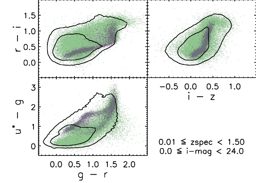
Figure 7.— Coverage of the color-color space by our spectroscopic samples. Magenta and green dots show our NGVSLenS and CFHTLenS spectroscopic samples, respectively. Contours represent the 68% and 95% loci of our NGVSLenS/phot24 photometric sample. Our spectroscopic samples satisfactorily cover the colors of the photometric sample.

5.2. Comparison with spec-z’s

We analyze in this section how our estimated photo-z’s compare with our spectroscopic sample. We use the full spectroscopic sample (NGVSLenS and CFHTLenS) in the redshift range $0.01\leq z_{\rm spec}<1.5$, without any selection in magnitude. For each object in our spectroscopic sample, we calculate $\Delta z=\frac{z_{\rm phot}-z_{\rm spec}}{1+z_{\rm spec}}$ and classify it as an outlier if $|\Delta z|>0.15$. For each considered sample, we report bias: the median value of $\Delta z$; outl.: the percentage of outliers; and $\sigma_{\rm outl.rej.}$: the standard deviation of $\Delta z$ when outliers have been excluded. These quantities are used to facilitate comparison with other works; as mentioned in Hildebrandt et al. (2012), the outlier definition is arbitrary.

Figure 8.— Photo-z’s with $u^{*}griz$ bands with Le Phare (left panel, red) and bpz (right panel, blue). Dark thick symbols represent the NGVSLenS spectroscopic sample (low redshift); light thin symbols represent the CFHTLenS spectroscopic sample (high redshift). We highlight with black crosses the NGVSLenS Keck subsample.

We present in Figure 8 how our photo-z’s compare with spec-z’s for our two spectroscopic samples and for both codes, Le Phare (left panel, in red) and bpz (right panel, in blue). The NGVSLenS objects (low redshift) are in thick dark symbols and the CFHTLenS objects (high redshift) are in thin light symbols.

At first sight, we see that both codes provide satisfactory photo-z’s over the range $0.1\lesssim z_{\rm spec}\lesssim 1$ and that the overall behavior of our spectroscopic samples over the NGVSLenS and the CFHTLenS fields is consistent in the overlap regions. We notice that, although statistically small, the NGVSLenS Keck subsample has photo-z’s in broad agreement with the other NGVSLenS subsamples and with the CFHTLenS spectroscopic sample, strengthening our choice of using the CFHTLenS data at high redshift.

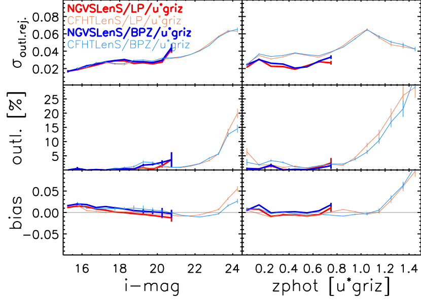
Figure 9.— Statistics for photo-z’s (estimated with $u^{*}griz$ bands) as a function of magnitude (left panel) and redshift (right panel). Photo-z’s estimated with Le Phare are in red and those estimated with bpz are in blue. Dark thick lines represent the NGVSLenS spectroscopic sample (low redshift); light thin lines represent the CFHTLenS spectroscopic sample (high redshift). We report quantities only for the bins where we have more than 50 galaxies. Error bars are calculated assuming a Poissonian distribution. Our photo-z’s estimated with the $u^{*}griz$-bands are more accurate for $i\lesssim 23$ mag or $z_{\rm phot}\lesssim 1$.

We show in Figure 9 a quantitative analysis of how the three quantities bias, $\sigma_{\rm outl.rej.}$, and outl. depend on the measured magnitude and the estimated photo-z.

First, we observe that the two codes (bpz and Le Phare) and the two datasets (NGVSLenS and CFHTLenS) provide consistent behavior over our tested ranges in magnitude or photo-z. This observation a posteriori validates our assumption, namely that the NGVSLenS and CFHTLenS data have very similar properties. However, when looking at the $\sigma_{\rm outl.rej.}$ as a function of photo-z, there is a clear difference between the NGVSLenS and CFHTLenS samples, which arises from the nature of the two spectroscopic samples in a given range. In the $0.3\lesssim z_{\rm phot}\lesssim 0.6$ range, the NGVSLenS sample has a significantly smaller $\sigma_{\rm outl.rej.}$. This is a direct consequence being of our NGVSLenS spectroscopic sample in this redshift range is highly biased towards LRGs. These galaxies have on average brighter magnitudes and smaller photometric errors (e.g., better defined 4,000 Å  break than the average galaxy), thus making the photo-z estimation easier. For instance, the typical value of the $i$-band magnitude at redshift $\sim$0.5 is 19.5 mag for our NGVSLenS spectroscopic sample versus 21.5 mag for our CFHTLenS spectroscopic sample (see right panel of Figure 6): a direct consequence is that the prior for those LRGs is significantly more peaked and at lower redshifts, thus constraining more the posterior. Indeed, as illustrated in Figure 10, the [0.11,0.65] redshift interval includes 95% of the prior for an elliptical galaxy with $i=19.5$ mag, whereas for an elliptical galaxy with $i=21.5$ mag the corresponding redshift interval is [0.14,1.00].

Another trend that illustrates this point is the outlier rate at $z_{\rm phot}\lesssim 0.2$: the CFHTLenS sample has 3-5% outliers against $<$1% for the NGVSLenS sample. Again, this can be explained by the characteristic $i$-band magnitude in this redshift range: when considering objects with $z_{\rm phot}<0.2$, only 5% of the NGVSLenS sample has $i>20$ mag against 27% for the CFHTLenS sample. The fainter galaxies of the CFHTLenS will have a much broader prior, hence the photo-z will be less constrained.

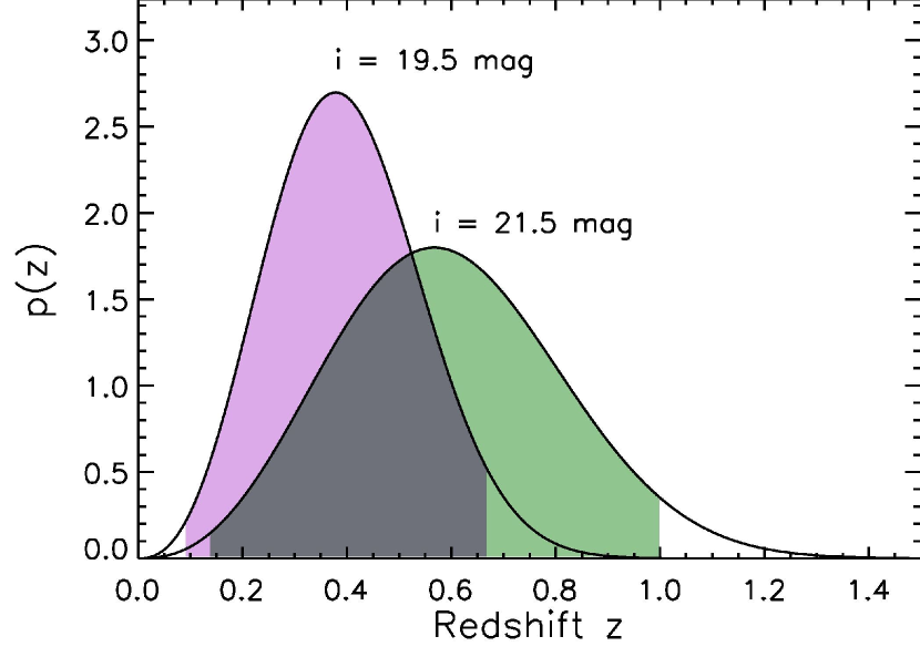
Figure 10.— Example of the prior for an elliptical template for two magnitudes representative of our spectroscopic samples at a redshift of $z\sim 0.5$: $i=19.5$ mag (in magenta, representative of our NGVSLenS spectroscopic sample) and $i=21.5$ mag (in green, representative of our CFHTLenS spectroscopic sample). The shaded areas enclose 95% of the prior. As a consequence, brighter galaxies will have on average sharper posteriors.

The quality of our photo-z’s decreases with increasing magnitude or redshift. For instance, with both codes, the $bias$ becomes significant ($>0.02$) for faint ($i\gtrsim 23$ mag) or high-z ($z\gtrsim 1.2$) objects, and the $\sigma_{\rm outl.rej.}$ goes from $\sim$0.02 for bright/low-z objects to $\sim$0.06 for faint/high-z objects. For $z_{\rm phot}\gtrsim 1.2$, our optical data do not bracket the 4,000 Å  break, and the photo-z’s are less reliable.

The quality of our photo-z for $i\gtrsim 17.5$ mag is consistent with that from the CFHTLenS data computed with Le Phare (Ilbert et al. 2006; Coupon et al. 2009) or with bpz (Hildebrandt et al. 2012; Erben et al. 2013). However, we obtain more robust photo-z’s down to at least $i\simeq 15.5$ mag because of the new prior that we introduce for the brightest galaxies.

5.3. Individual photo-z uncertainty $z_{\rm phot,err.}$

In this section we discuss the individual photo-z uncertainty estimation, which we label $z_{\rm phot,err.}$. For Le Phare, we use Z_ML68_LOW and Z_ML68_HIGH, which represent for each galaxy the boundary of the interval including 68% of the redshift probability distribution function; bpz provides only 95% uncertainty on $z_{\rm phot}$: for each object, we compute, based on the output posterior, the 68% confidence interval as defined in Le Phare.

In the top panels of Figure 11, we present the percentage of objects having $z_{\rm spec}$ within $z_{\rm phot}\pm z_{\rm phot,err.}$, for our spectroscopic sample and as a function of measured magnitude or photo-z. On average, this percentage is close to $68\%$, which means that our estimated individual $z_{\rm phot,err.}$ are realistic.

We see a departure from this behavior for the NGVSLenS sample at $i\gtrsim 20$ mag and at $z_{\rm phot}\gtrsim 0.5$: this is again due to the fact that our NGVSLenS spectroscopic sample in this magnitude/redshift range is highly biased towards LRGs. Indeed, as those objects are bright with a clear 4,000 Å  break, the estimated individual $z_{\rm phot,err.}$ is small, hence the $z_{\rm spec}$ can be outside of the $z_{\rm phot}\pm z_{\rm phot,err.}$ interval. This means that the uncertainties obtained for the photometric redshift are underestimated for LRGs: for this population, setting a minimal value of 0.04 for $z_{\rm phot,err.}$ allows to recover realistic errors.

In the lower panels of Figure 11 we present how the median value of $z_{\rm phot,err.}$ varies as a function of the measured magnitude and $z_{\rm phot}$. The median value of $z_{\rm phot,err.}$ depends strongly on magnitude. The grey area shows the region including the 68% of our NGVSLenS/phot24 sample photometric sample. For the spectroscopic sample, the median value of $z_{\rm phot,err.}$ is comparable to the scatter $\sigma_{\rm outl.,rej.}\times(1+z_{\rm spec})$ for $i<23$ mag or $z_{\rm phot}<1$ (i.e., when the factor $(1+z_{\rm spec})$ is taken into account). Our spectroscopic sample is representative of the overall behavior of all photometric objects, even if the spectroscopic sample has lower median uncertainties as a function of redshift, because the majority of the photometric sample includes objects fainter than the spectroscopic sample ($i>22$ mag).

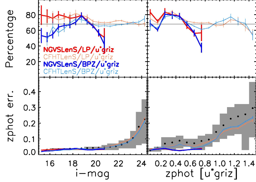
Figure 11.— Properties of, $z_{\rm phot,err.}$, the individual error estimation on the photo-z (estimated with $u^{*}griz$ bands) as a function of magnitude (left panel) and redshift (right panel). Photo-z’s estimated with Le Phare are in red and those estimated with bpz are in blue. Dark thick lines represent the NGVSLenS spectroscopic sample (low redshift); light thin lines represent the CFHTLenS spectroscopic sample (high redshift). Error bars are calculated assuming a Poissonian distribution. Top panels: percentage of objects having $z_{\rm spec}$ within $z_{\rm phot}\pm z_{\rm phot,err.}$. The fact that these percentages are close to $68\%$, as expected from the $z_{\rm phot,err.}$ uncertainty estimation, means that our estimated $z_{\rm phot,err.}$ are realistic. Bottom panels: median value of $z_{\rm phot,err.}$ (the continuous red and blue line are for Le Phare and bpz, respectively); for each bin along the x-axis, the black dots represent the median value of $z_{\rm phot,err.}$ for photometric objects in our NGVSLenS/phot24 sample and the grey shaded areas represent the regions enclosing $68\%$ of their distribution. Our spectroscopic sample is representative of the photometric sample.

5.4. Photo-z’s without the $r$-band

As mentioned in Section 2, a majority (83/117 fields) of the NGVSLenS field has not been imaged yet with the $r$-band. In this Section, we present the quality of our photo-z’s when the $r$-band is not available. To estimate it, we re-calculated the photo-z’s using only the $u^{*}giz$-bandpasses for the 34 NGVSLenS fields having $r$-band coverage, and for the CFHTLenS fields, thus using our full spectroscopic sample ($\sim$83,000 galaxies).

Figs. 12 and 13 summarize the properties of the photo-z’s for our spectroscopic sample when the $r$-band is missing. We also present in Figure 14 the comparison of the statistics for the photo-z’s estimated with or without the $r$-band for our CFHTLenS spectroscopic sample. In our CFHTLenS spectroscopic sample, our photo-z’s are more scattered in the $0.3\lesssim z_{\rm spec}\lesssim 0.8$ range, where the $r$-band filter is essential to constrain the 4,000 Å  break. This effect is less pronounced for our NGVSLenS spectroscopic sample because, as discussed in Section 5.2 (see also Figure 10), our NGVSLenS spectroscopic sample is highly biased towards LRGs (i.e., thus not representative of the general galaxy population) in this redshift range: the prior – more peaked and at lower redshift than for average galaxies at similar redshift – helps to obtain fewer false values for the posterior. When we compare the statistics, (e.g., Figure 13 with Figure 9), when the $r$-band is missing the outliers rate increases significantly in the $0.3\lesssim z_{\rm phot}\lesssim 0.8$ range and peaks at $\sim$10-15%. We remark that the overall behavior of the two codes is similar.

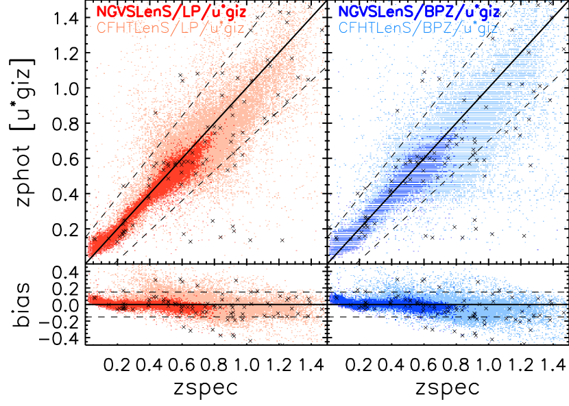
Figure 12.— Photo-z’s with $u^{*}giz$ bands with Le Phare (left panel, red) and bpz (right panel, blue). Dark thick symbols represent the NGVSLenS spectroscopic sample (low redshift); light thin symbols represent the CFHTLenS spectroscopic sample (high redshift). We highlight with black crosses the NGVSLenS Keck subsample.

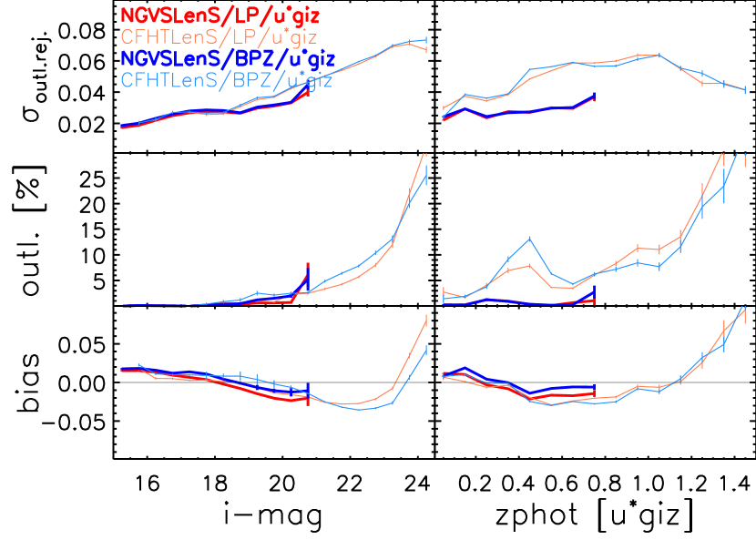
Figure 13.— Statistics for photo-z’s (estimated with $u^{*}giz$ bands) as a function of magnitude (left panel) and redshift (right panel). Photo-z’s estimated with Le Phare are in red and those estimated with bpz are in blue. Dark thick lines represent the NGVSLenS spectroscopic sample (low redshift); light thin lines represent the CFHTLenS spectroscopic sample (high redshift). We report quantities only for the bins where we have more than 50 galaxies. Error bars are calculated assuming a Poissonian distribution. When the $r$-band is missing the quality of our photo-z’s decreases for the three plotted quantities in the $0.3\lesssim z_{\rm phot}\lesssim 0.8$ range and in the $i\gtrsim 21$ mag range (bias, outl., and $\sigma_{\rm outl.rej.}$ can increase of more than 100%).

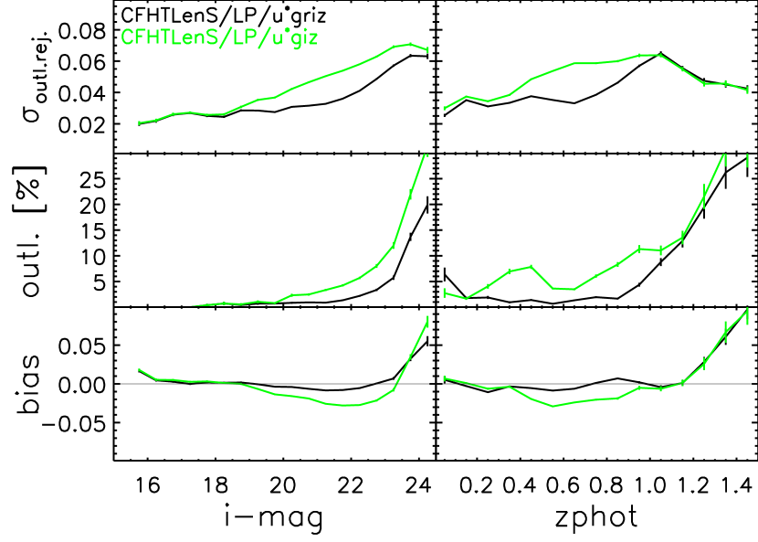
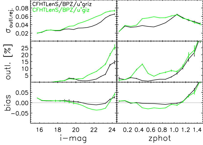
Figure 14.— Statistics for photo-z’s estimated with Le Phare (left) and with bpz (right), as a function of magnitude and redshift, for our CFHTLenS spectroscopic sample. Photo-z’s estimated with the $u^{*}griz$ bands are in black and those estimated with the $u^{*}giz$ bands are in green. We report quantities only for the bins where we have more than 50 galaxies. Error bars are calculated assuming a Poissonian distribution. When the $r$-band is missing the quality of our photo-z’s decreases for the three plotted quantities in the $0.3\lesssim z_{\rm phot}\lesssim 0.8$ range and in the $i\gtrsim 21$ mag range (bias, outl., and $\sigma_{\rm outl.rej.}$ can increase of more than 100%).

The observation that the photo-z quality decreases in the $0.3\lesssim z_{\rm spec}\lesssim 0.8$ range is supported only by our CFHTLenS spectroscopic sample. Using the results of Section 5.2, we can assume that our photo-z’s estimated with five bands $u^{*}griz$ are unbiased down to $i<23$ mag. Under this assumption, we can use our NGVSLenS/phot23 sample (see Section 5.1 and Table 5.1), i.e., the whole NGVSLenS photometric sample with $i<23$ mag and covered by the five bands, to probe how photometric redshifts change if the $r$-band is missing.

Figure 15 compares the photo-z’s estimated with $u^{*}giz$ bands versus those estimated with the $u^{*}griz$ bands, for the two codes and by magnitude bins. We consider here objects from our NGVSLenS/phot23 photometric sample, thus $5.8\times 10^{5}$ objects. It confirms the result obtained with the CFHTLenS spectroscopic sample, which is that a significant number of objects with $0.3\lesssim z_{\rm phot}\lesssim 0.8$ are outliers.

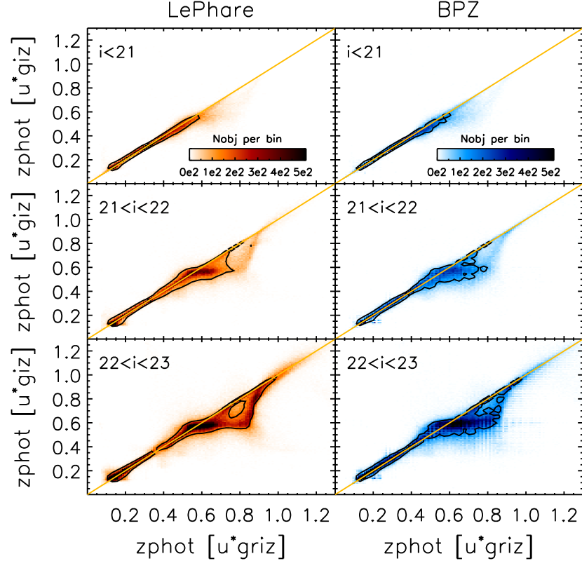
Figure 15.— Photo-z’s with $u^{*}giz$ bands vs. photo-z’s with $u^{*}griz$ bands for our NGVSLenS/phot23 photometric sample, by magnitude bins. Left column: photo-z’s estimated with Le Phare; right column: photo-z’s estimated with bpz. We represent the density of objects per 0.01$\times$0.01 bin in $z_{\rm phot}$. Black contours represent the loci enclosing 68% of the distribution. The analysis with a large NGVSLenS photometric sample confirms the one done with the CFHTLenS spectroscopic sample.

Under the same assumption – our photo-z’s estimated with the $u^{*}griz$ bands are globally unbiased down to $i<23$ mag – we can produce a plot similar to Figure 13, but using our NGVSLenS/phot23 photometric sample, as above. In Figure 16, we present the statistics for our photo-z’s estimated with the $u^{*}giz$ bands, using the photo-z’s estimated with the $u^{*}griz$ bands as a proxy of $z_{\rm spec}$. Most of the features of Figure 13 are rather accurately reproduced with this sample of $5.8\times 10^{5}$ photometric objects. These statistics are dominated by faint galaxies, and less biased by the LRGs, and are consistent with statistics obtained with the CFHTLenS spectroscopic sample.

Figure 16 strengthens the results shown in Figure 13, as the statistics are closely reproduced by using a sample of $5.8\times 10^{5}$ photometric objects.

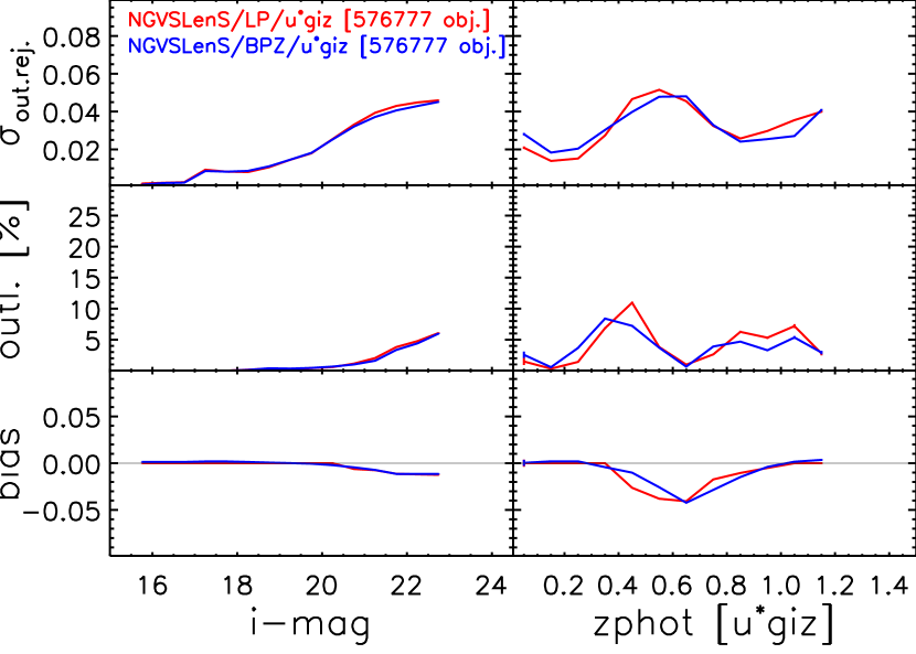
Figure 16.— Statistics for photo-z’s (estimated with $u^{*}giz$ bands) in our NGVSLenS/phot23 photometric sample ($>$$5\times 10^{5}$ objects), as a function of magnitude (left panel) and redshift (right panel). Photo-z’s estimated with Le Phare are in red and those estimated with bpz are in blue. Figure similar to Figure 13, but the spectrospic sample has been replaced by a NGVSLenS photometric sample ($5.8\times 10^{5}$ objects) and the spec-z’s have been replaced by the photo-z’s estimated with the $u^{*}griz$ bands. Error bars, calculated assuming a Poissonian distribution, are not visible because of the large size of the sample. The analysis with a large NGVSLenS photometric sample confirms the one done with the CFHTLenS spectroscopic sample.

5.5. Joint analysis of photo-z dependence on magnitude and redshift

The above analysis shows that the photo-z’s statistics can be biased by the properties of the spectroscopic sample chosen as reference. Indeed, the galaxies selected as targets for spectroscopic samples might have properties that are not characteristic of the entire photometric sample. In particular, spectroscopic samples are dominated by brighter galaxies that represent a small percentage of the entire photometric samples, at a given redshift. This means that fainter galaxies, which statistically dominate the photometric sample, will not be correctly represented in the spectroscopic sample. In our case, we do have spectroscopic samples that cover the fainter magnitudes (see Figure 6, bottom panel), however at a given redshift they include significantly fewer galaxies than those that cover the bright end, which dominate our statistics shown in previous sections.

Moreover, as shown in Figure 6, our spectroscopic samples cover different ranges in redshift and magnitude and, when binning only in magnitude or in redshift, we are mixing galaxies that have very different properties.

For those reasons, we here separate different magnitude bins at a given redshift, and perform a joint analysis in enough small bins of redshift and magnitude, in which we can select galaxies with similar properties.

In Figure 17 and in Table 5, we present a joint analysis in redshift and magnitude on the entire NGVSLenS and CFHTLenS spectroscopic samples ($\sim$83,000 galaxies). We have already discussed that Le Phare and bpz provide photo-z’s with similar properties and, for simplicity, we present only Le Phare photo-z’s for this analysis. When using bpz, our results do not change.

This analysis clarifies what has been observed in the previous sections and refines the conclusions. In a given redshift bin, the quality of the photo-z’s depends on magnitude, with fainter galaxies having more uncertain photo-z’s estimates. Bright galaxies with $i<21$ mag have accurate photo-z’s, independent of redshift. Their bias and scatter are low ($|bias|<0.02$ and $\sigma_{\rm outl.rej.}<0.04$) and they have a small number of outliers ($<6\%$). This also true when the photo-z’s are estimated without the $r$-band for $i<20$ mag. For fainter galaxies ($i>21$ mag), it results in a steeper decline in the accuracy of the photo-z estimate as a function of magnitude in the $0.3\lesssim z_{\rm phot}\lesssim 0.8$. As previously explained, this depends on tighter priors on the brightest galaxies, and on the predominance of galaxies with more defined 4,000 Å  breaks at the higher end of the luminosity function.

At fixed magnitude, photo-z estimates at higher redshift are often more accurate, just because we are probing galaxies with higher absolute luminosity, e.g. intrinsically brighter galaxies at higher redshift, that will have more defined 4,000 Å  breaks. When the optical bandpasses no longer bracket the 4,000 Å  break ($z\gtrsim 1.2$), this is no longer true and the photo-z’s become more uncertain even for bright red sequence galaxies.

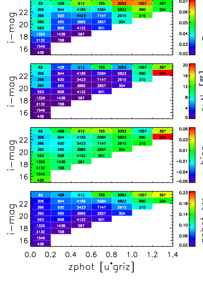
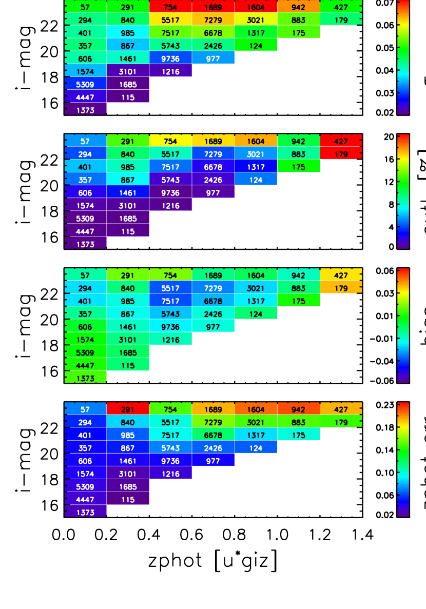
Figure 17.— Joint analysis of our photo-z’s estimated with Le Phare and the $u^{*}griz$-bands (left panel) and the $u^{*}giz$-bands (right panel). From top to bottom, we display $\sigma_{\rm outl.rej.}$, outl., bias, and the median value of $z_{\rm phot,err.}$. We use here our full spectroscopic sample (NGVSLenS and CFHTLenS; $\sim$83,000 galaxies). The statistics are presented by binning it both in magnitude and photo-z. We only display the bins where we have more than 50 galaxies and, for those bins, we report the number of galaxies used to compute the statistics.

Table 5Photo-z (estimated with Le Phare) properties for our compiled spectroscopic sample (NGVSLenS and CFHTLenS).

Binning				$u^{*}griz$-bands						$u^{*}giz$-bands
$i^{\rm min}$	$i^{\rm max}$	$z_{\rm phot}^{\rm min}$	$z_{\rm phot}^{\rm max}$	bias	$\sigma_{\rm outl.rej.}$	outl.	$z_{\rm phot,err.}$	Ngal	zSurvey†	bias	$\sigma_{\rm outl.rej.}$	outl.	$z_{\rm phot,err.}$	Ngal	zSurvey†
[mag]	[mag]					[%]						[%]
15.0	16.0	0.0	0.2	0.01	0.02	0	0.03	438	A	0.02	0.02	0	0.03	1373	A
16.0	17.0	0.0	0.2	0.01	0.02	0	0.03	1549	A	0.01	0.02	0	0.03	4447	A
16.0	17.0	0.2	0.4	$\cdots$	$\cdots$	$\cdots$	$\cdots$	$\cdots$	$\cdots$	0.00	0.02	0	0.02	115	A
17.0	18.0	0.0	0.2	0.01	0.03	0	0.04	2132	A	0.01	0.03	0	0.04	5309	A
17.0	18.0	0.2	0.4	0.00	0.02	0	0.03	708	D	0.00	0.02	0	0.02	1685	D
18.0	19.0	0.0	0.2	0.00	0.03	0	0.04	1326	B	0.01	0.03	1	0.04	1574	B
18.0	19.0	0.2	0.4	0.00	0.02	1	0.03	1438	D	-0.01	0.02	0	0.03	3101	D
18.0	19.0	0.4	0.6	0.00	0.02	0	0.03	587	D	-0.01	0.02	0	0.04	1216	D
19.0	20.0	0.0	0.2	0.00	0.04	2	0.04	593	C	0.00	0.04	2	0.04	606	C
19.0	20.0	0.2	0.4	-0.01	0.03	1	0.05	808	D	-0.01	0.04	3	0.04	1461	D
19.0	20.0	0.4	0.6	0.00	0.02	0	0.03	4122	D	-0.02	0.03	0	0.05	9736	D
19.0	20.0	0.6	0.8	0.00	0.03	2	0.04	901	D	-0.01	0.03	1	0.05	977	D
20.0	21.0	0.0	0.2	-0.01	0.04	6	0.04	360	E	-0.01	0.04	5	0.05	357	E
20.0	21.0	0.2	0.4	-0.02	0.03	2	0.05	695	H	-0.02	0.04	7	0.05	867	H
20.0	21.0	0.4	0.6	-0.01	0.03	0	0.04	3885	F	-0.02	0.04	1	0.07	5743	F
20.0	21.0	0.6	0.8	0.00	0.03	1	0.04	2857	F	-0.01	0.04	1	0.07	2426	F
20.0	21.0	0.8	1.0	0.01	0.04	1	0.06	304	F	0.00	0.05	5	0.07	124	F
21.0	22.0	0.0	0.2	-0.02	0.04	6	0.04	396	H	-0.02	0.04	6	0.05	401	E
21.0	22.0	0.2	0.4	-0.02	0.03	2	0.06	920	E	-0.01	0.04	8	0.07	985	H
21.0	22.0	0.4	0.6	-0.01	0.03	1	0.06	5423	F	-0.04	0.05	5	0.10	7517	F
21.0	22.0	0.6	0.8	-0.01	0.03	1	0.05	7147	F	-0.02	0.05	2	0.12	6678	F
21.0	22.0	0.8	1.0	0.00	0.04	1	0.07	2915	F	-0.02	0.05	3	0.09	1317	F
21.0	22.0	1.0	1.2	0.01	0.05	8	0.10	215	F	0.01	0.05	11	0.10	175	F
22.0	23.0	0.0	0.2	-0.02	0.04	7	0.05	306	H	-0.02	0.04	4	0.05	294	H
22.0	23.0	0.2	0.4	-0.01	0.04	1	0.07	844	H	0.00	0.04	10	0.09	840	H
22.0	23.0	0.4	0.6	-0.01	0.04	1	0.07	4185	F	-0.03	0.06	8	0.10	5517	F
22.0	23.0	0.6	0.8	0.00	0.04	2	0.08	5584	F	-0.03	0.06	4	0.16	7279	F
22.0	23.0	0.8	1.0	0.01	0.05	1	0.09	5823	F	-0.02	0.06	5	0.15	3021	F
22.0	23.0	1.0	1.2	0.00	0.05	9	0.12	990	F	0.00	0.05	9	0.15	883	F
22.0	23.0	1.2	1.4	0.06	0.05	32	0.14	204	F	0.04	0.04	31	0.15	179	F
23.0	24.0	0.0	0.2	-0.01	0.04	8	0.07	62	H	-0.01	0.05	5	0.07	57	H
23.0	24.0	0.2	0.4	0.00	0.04	4	0.08	428	G	0.02	0.05	13	0.64	291	H
23.0	24.0	0.4	0.6	0.02	0.05	6	0.09	912	H	0.02	0.07	16	0.15	754	H
23.0	24.0	0.6	0.8	0.02	0.05	10	0.15	765	H	0.00	0.07	16	0.20	1689	H
23.0	24.0	0.8	1.0	0.02	0.06	6	0.12	2093	H	0.00	0.07	17	0.21	1604	H
23.0	24.0	1.0	1.2	-0.01	0.06	10	0.17	1057	H	-0.01	0.06	10	0.22	942	H
23.0	24.0	1.2	1.4	0.03	0.05	14	0.18	397	H	0.04	0.05	20	0.20	427	H

Note. — We report quantities only for the bins where we have more than 50 galaxies.

^†: Spectroscopic survey from which the majority of the galaxies in the considered bin originates: A:SDSS/Galaxy Main Sample, B:E.Peng/AAT, C:E.Peng/Hectospec, D:SDSS/other programs, E:VVDS/F22, F:VIPERS, G:VVDS/F02, H:DEEP2/EGS.

6. Angular correlation function

A complementary way to test the photo-z accuracy using the whole NGVSLenS sample, is to calculate the galaxy angular correlation function, ($w(\theta)$; e.g., Newman 2008; Hildebrandt et al. 2009a; McQuinn & White 2013), in different redshift bins. The advantage of this approach is that we probe the photo-z directly on the NGVSLenS data, and do not have to make assumption about the spectroscopic samples we are using. This permits an estimation of the level of contamination between photometric redshift bins. As a result of galaxy clustering, the angular correlation in a given redshift bin (auto-correlation) should be positive on small scales when compared to a random distribution of points; on large scales, the angular auto-correlation should tend to zero. When looking at two redshift bins, the angular correlation (cross-correlation) should be zero if the redshift bins are well separated, since the galaxies are physically separated by large distances; if the considered redshift bins are close to each other and have sizes close to the typical photo-z uncertainty, this produces a non-zero cross correlation. We refer to Erben et al. (2009) for a detailed presentation of the angular correlation function formalism.

We apply the pairwise analysis using the publicly available athena tree code on our NGVSLenS data in redshift bins defined by the following limits: $z_{cut}=0.1;0.2;0.3;0.4;0.5;0.6;0.7;0.8;0.9;1.0;1.2$. Note that we neglect the effects of magnification (Scranton et al. 2005; Hildebrandt et al. 2009b). We do not consider the range $0\leq z<0.1$, as it contains too few objects (few thousands) to estimate robust statistics. We only consider objects having $i<23$ mag, not classified as star or GC (see Appendix C). To exclude galaxies with unreliable $z_{\rm phot}$, we exclude galaxies with $z_{\rm phot,err.}>0.25$ (according to Figure 11, the 3$\sigma$ upper limit of $z_{\rm phot,err.}$ at $i=23$ mag is 0.25). Also excluding all masked areas and field edges (to prevent duplicates when merging the fields), we end up with $4\times 10^{5}$ objects when using photo-z’s derived from $u^{*}griz$ bands, and $1.1\times 10^{6}$ objects with just $u^{*}giz$ filters. To compare with a random distribution, we generate random catalogs, having uniformly distributed positions with the same geometry as our NGVSLenS data (imaged areas and masks). Because our chosen bin widths are at worse about twice as large than our photo-z scatter ($\sigma_{\rm outl.rej.}\lesssim 0.06$), we expect a low-level cross-correlation signal in neighboring redshift bins, and a $w(\theta)$ compatible with zero for bins distant in redshift.

Figure 18 shows $w(\theta)$ for the photo-z’s estimated with the $u^{*}griz$ bands and Le Phare. The figure – hence the conclusions – is similar if we use bpz or if we use the $u^{*}giz$ bands. This figure is consistent with the expected behavior, which is a positive signal for auto-correlation (diagonal panels, in blue) and a signal consistent with zero for cross-correlation (red panels), except for adjacent redshift windows (second panel of each line, rightward of the blue panels) and for the second off-diagonal panels at small scales (third panel of each line). A signal consistent with zero for cross-correlation in distant redshift bins confirms that our levels of contamination are minimal, as found in our previous analysis with spectroscopic samples.

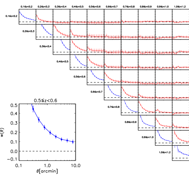
Figure 18.— Angular correlation for objects with $0.1<z_{\rm phot}\leq 1.2$, $i<23$ mag, $z_{\rm phot,err.}\leq 0.25$, not classified as star or GC, and covered by the $u^{*}rgiz$ bands, split by redshift bins. Photo-z’s have been estimated with Le Phare. The bottom left panel is a zoom-in to the corresponding panel of the matrix plot. The absence of positive angular correlation in distant redshift bins is consistent with independent photometric redshift measurements.

7. Conclusions

We present an analysis of the determination of the photo-z catalog for the NGVS survey. This survey images 104 deg² around the Virgo cluster with the $u^{*}giz$-bands, amongst which 34 pointings have $r$-band coverage. To obtain good quality matched photometry, we used an upgraded version of the theli pipeline developed for the analysis of the CFHTLenS data, which have properties very similar to our data. The theli pipeline products are the co-added astrometrically and photometrically calibrated images for all the NGVSLenS pointings in each filter, the photometric catalogs, and the photo-z catalogs.

We uniformly calibrated the photometry using the SDSS, which covers the full NGVSLenS. We built photometric catalogs from the multi–wavelength images convolved to the same seeing on each field. This PSF homogenization allows an accurate measurement of colors, which is fundamental to obtain precise photo-z’s. We paid particular attention to the magnitude uncertainty estimation, accounting for the convolution process. We estimate the photo-z’s with two template fitting codes, Le Phare and bpz. We extended the prior of those codes to bright objects (seven magnitudes brighter), thus being able to accurately estimate photo-z’s over a large range of magnitudes.

To assess the quality of our photo-z catalog, we used a large spectroscopic sample ($\sim$83,000 galaxies) in the $0.01\leq z_{\rm spec}<1.5$ and $15.5\leq i\leq 24.5$ mag ranges. We presented a detailed analysis of our photo-z’s as a function of the measured magnitude, redshift, and the number of bandpasses used for their estimation ($u^{*}griz$ or $u^{*}giz$).

Our analysis concluded that both codes perform very similarly. When using the $u^{*}griz$ bands, we obtain accurate photo-z’s for $i\lesssim 23$ mag or $z_{\rm phot}\lesssim 1$: the bias is reasonable ($|bias|<0.02$), the scatter $\sigma_{outl.rej}$ increases with the magnitude (from 0.02 to 0.05 for $i$ in [15.5,23]), and the outliers represent less than 5% of the sample. For photo-z’s estimated without the $r$-band (i.e., with the $u^{*}giz$ bands), the accuracy decreases slightly. The lack of $r$-band results in more pronounced uncertainties in the $0.3\lesssim z_{\rm phot}\lesssim 0.8$ range, where it samples the 4,000 Å  break. In this redshift range, we have $-0.05<bias<-0.02$, $\sigma_{outl.rej}\sim 0.06$ and an outlier rate that peaks at 10-15%. The quality of photo-z’s estimated with the $u^{*}giz$ bands also decreases at $i>21$ mag. However, we remark that the brightest galaxies, e.g. the LRGs which constitute the main part of our NGVSLenS spectroscopic sample at $0.3<z_{\rm spec}<0.8$, have photo-z’s of almost similar quality than when the $r$-band is used (but a slightly higher bias). This is because of the different typical magnitudes of the LRGs with respect of the average galaxy in a given redshift bin: these galaxies have tighter priors because they are the brightest at a given redshift, and have a well defined 4,000 Å  break. Our results are visualized and interpreted in a joint analysis in magnitude and redshift bins.

Finally, we presented an analysis of the angular correlation function $w(\theta)$, to internally assess the quality of our photo-z’s using the whole NGVSLenS sample with $i\leq 24$ mag and $0.1\leq z_{\rm phot}\leq 2$. We obtain results that are consistent with expectations, i.e., a positive signal for auto-correlation (decreasing with increasing angle) and a signal consistent with zero for cross-correlation when considering redshift bins with a redshift separation greater than 0.1.

The NGVSLenS catalogs will be public on June, 1st 2015 on the NGVS website. Before that date, please contact us if you would like to use them .

Appendix A Prior extension to bright objects

Le Phare and BPZ were designed for high redshift studies. Both codes use similar priors for $i>20$ mag galaxies (calibrated with $\sim$1,300 galaxies for BPZ and with $\sim$6,500 galaxies for Le Phare), and for $i<20$ mag a prior that is not calibrated on observed data. As a result of the large area covered by the NGVSLenS, $i<20$ mag galaxies represent a non-negligible fraction of our sample. We thus build a new prior calibrated for bright and faint objects. Our estimated parameters are displayed in Table 6.

Table 6Prior used in this article.

Spectral	$i_{ref}$	$\alpha_{t}$	$z_{0t}$	$k_{mt}$	$f_{t}$	$k_{t}$
template type $T$
$i_{AB}\leq 12.5$
$p(z)\propto 1$ if $z<0.1$, $p(z)=0$ else
$12.5<i_{AB}\leq 17$
Ell	12.5	2.46	0	0.027	0.86	0.062
Spi	12.5	2.07	0	0.021	0.14	-0.108
Irr	12.5	1.89	0	0.015	…	…
$17<i_{AB}\leq 20$
Ell	17.0	2.46	0.121	0.103	0.65	0.257
Spi	17.0	1.94	0.095	0.098	0.23	-0.014
Irr	17.0	1.95	0.069	0.077	…	…
$20<i_{AB}$
Ell	20.0	2.46	0.431	0.091	0.30	0.40
Spi	20.0	1.81	0.390	0.100	0.35	0.30
Irr	20.0	2.00	0.300	0.150	…	…

According to the formalism introduced in Benítez (2000) and using our template set (see Section 4.2 and Table 3), for a galaxy with an $i$-band magnitude $i_{AB}$, the a priori probability of having a redshift $z$ and a spectral template type $T$ is:

$$p(z,T|i_{AB})=p(T|i_{AB})\times p(z|T,i_{AB}).$$ (A1)

$p(T|i_{AB})$ is the probability for a galaxy of magnitude $i_{AB}$ to have a spectral template type $T$ and is parametrized as:

$$p(T|i_{AB})\propto f_{t}\times\textnormal{exp}\left(-k_{t}\times\left[i_{AB}-i_{ref}\right]\right).$$ (A2)

$p(z|T,i_{AB})$ is the probability for a galaxy of magnitude $i_{AB}$ and spectral template type $T$ to have a redshift $z$ and is parametrized as:

$$p(z|T,i_{AB})\propto z^{\alpha_{t}}\times\textnormal{exp}\left(-\left[\frac{z}{z_{0t}+k_{mt}\times(i_{AB}-i_{ref})}\right]^{\alpha_{t}}\right).\\$$ (A3)

$i_{ref}$ is a reference magnitude.

For galaxies with $i>20$ mag, we use the Le Phare prior, calibrated on the robust VVDS spectroscopic sample. For galaxies with $12.5<i\leq 17$ mag, we calibrate our prior with the SDSS spectroscopic Galaxy Main Sample (York et al. 2000; Strauss et al. 2002), using the DR10 release (Ahn et al. 2014). We select objects with class$=$GALAXY and use cModelMag_i as $i$-band total magnitude and ModelMag quantities to compute colors (we correct for extinction). This sample is complete down to $r\leq 17.77$ mag, thus complete down to $i\sim 17$ mag (in fact, most of the galaxies with $r\leq 17.77$ mag have $z\lesssim 0.4$, and for $z\lesssim 0.4$ the color $(r-i)\lesssim 0.8$; see Figure 5). For consistency with standard prior already implemented in BPZ and Le Phare, we follow the formalism of Benítez (2000) and define three broad spectral classes: Ellipticals (Ell template), Spirals (Sbc, Scd templates), and Irregulars (Im, SB2, SB3 templates). We associate each galaxy from the SDSS spectroscopic Galaxy Main Sample to one of those broad spectral classes, by using the best-fit template (from the photometric redshift code) when fixing the redshift at $z_{\rm spec}$. We thus have $\sim$320,000 galaxies with $12.5<i<17$ mag and classified into three broad spectral classes. We then fit with a least-square fitting method (IDL MPFIT package, Markwardt 2009) the fraction of each spectral type as a function of the magnitude with equation A2 and we obtain the $k_{t}$ parameter, and the redshift distribution of each spectral type T in each magnitude bin with equation A3 and obtain the $\alpha_{t}$, $z_{0t}$, $k_{mt}$ parameters. For $17<i\leq 20$ mag galaxies, we extrapolate the parameter values to match those fitted at $i_{AB}=17$ mag and $i_{AB}=20$ mag. For $\alpha_{t}$, we take the mean value of those estimated at $i_{AB}=17$ mag and $i_{AB}=20$ mag, and we set the other parameters so that the quantities $z_{0t}+k_{mt}\times(i_{AB}-i_{ref})$ and $f_{t}\times\textnormal{exp}(i_{AB}-i_{ref})$ are continuous. For $i\leq 12.5$ mag galaxies, we set a square prior, $p(z)$ being non-null for $z<0.1$ and null for $z\geq 0.1$.

To illustrate how our new prior improves the photo-z accuracy, we display in the right panel of Figure 19 the statistics for the photo-z estimated with $u^{*}griz$-bands and using Le Phare and BPZ original priors. When comparing with the Figure 9, we see that our new prior, for $i<20$ mag galaxies, improves significantly the bias and, to a lesser extent, the scatter and the percentage of outliers; as a consequence, it also improves the photo-z accuracy at $z_{\rm{phot}}<0.4$.

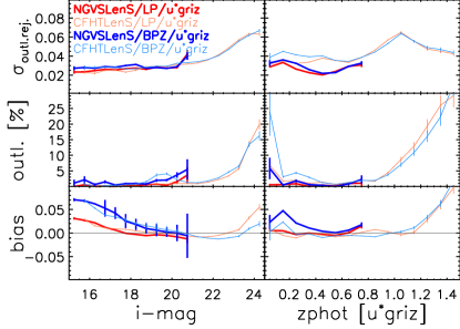
Figure 19.— Statistics for photo-z’s (estimated with $u^{*}griz$ bands) as a function of magnitude (left panel) and redshift (right panel), when using Le Phare and BPZ original priors. Symbols are similar to those in Figure 9. At $i<20$ mag, the bias is larger than when using our re-computed prior in Figure 9.

Appendix B Similarity of the NGVSLenS and CFHTLenS datasets

In Section 5, we assume that the CFHTLenS dataset – re-reduced with our changes in the theli pipeline – has similar properties as our NGVSLenS datasets. This is justified by the fact that both datasets have been obtained with the same telescope, instrument, and filterset, have by construction similar depth, and have been reduced with the same pipeline.

In this Section, we illustrate, a posteriori the similarity of the datasets resulting from these two surveys. We display in Figure 20 our estimated uncertainties in magnitude as a function of magnitude for both datasets. Each point represents the median value of the magnitude error for a given magnitude bin in each field. The crosses and error bars represent the global values for each survey (median and standard deviation of those individual – i.e., for each field – data).

We observe that two datasets have indeed very similar depths for all bands. The NGVSLenS has slightly better photometry in the $u^{*}$- and $z$-bands. We note the large standard deviations for the $r$-band for the NGVSLenS, that is due to the continuation of the NGVSLenS program for some fields with smaller exposure times (see Section 4.4 of Ferrarese et al. 2012).

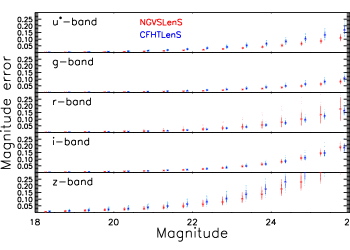
Figure 20.— Magnitude uncertainty as a function of magnitude for the NGVSLenS (red) and the CFHTLenS (blue) data, and for the $u^{*}griz$ bands. Each point represent the median values for a given field (i.e., 1 deg²). The crosses and error bars represent the global values for each survey (median and standard deviation of those individual – i.e., for each field – data). CFHTLenS data are offset by 0.1 mag along the x-axis to increase readability. Both datasets have very similar depths for all bands.

Appendix C Stars and Globular clusters removal

In the Figures using photometric samples, we exclude objects that are most probably stars or GCs. We describe in this Appendix the criteria we use to exclude those objects. For more detailed NGVS studies of stars and GCs, please refer to Lokhorst et al. (in preparation) and Durrell et al. (2014), respectively.

C.1. Stars removal

To separate stars from galaxies we follow a simple approach. We classify an object as a star if it satisfies: $\texttt{CLASS\_STAR}>0.95$ and $i<21.5$ mag, where CLASS_STAR is a SExtractor output quantifying the star/galaxy classification. To assess the efficiency of our classification, we have in hand $\sim$6,900 CFHTLenS spectroscopically identified stars ($i=20.7\pm 1.4$ mag; using the DEEP2/EGS, VVDS, and VIPERS) and $\sim$3,000 NGVSLenS spectroscopic stars ($i=18.9\pm 1.5$ mag; using the SDSS), and our galaxy spectroscopic samples (NGVSLenS and CFHTLenS; $\sim$83,000 galaxies with $0.01\leq z_{\rm spec}<1.5$).

We present in Figure 21 the percentage of stars correctly classified as stars (upper panel) and the percentage of galaxies misclassified as stars (bottom panel) when using our criteria. We correctly classify $>85\%$ of the stars with $i<21.5$ mag and misclassify as stars $<5\%$ of our galaxies. Note that, at $i=22$ mag, we expect galaxies to be about 10 times more numerous than stars (see Figure 3 of Lilly et al. 2007, for the COSMOS field, which lies at a Galactic latitude lower than the NGVSLenS), and even more at fainter magnitudes. Therefore, for $i>21.5$ mag objects, the number of stars should be marginal when compared to the number of galaxies and should not affect the statistics. The performance of our star/galaxy classification is thus satisfactory for our needs.

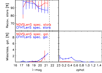
Figure 21.— Star/galaxy separation efficiency as a function of the $i$-band magnitude (left panel) or $z_{\rm phot}$ (right panel). The upper panel represent the percentage of stars correctly classified as stars; the lower panels represent the percentage of galaxies wrongly classified as stars. Please see text for description of the samples. The vertical dashed lines show the faint limit ($i=21.5$ mag) we use to assign the star classification. We report quantities only for the bins where we have more than 50 objects. Error bars are calculated assuming a Poissonian distribution.

C.2. Globular clusters removal

A special feature – and the main goal – of the NGVS is its full coverage of the Virgo cluster: a direct consequence is a massive detection of Globular Clusters (GCs). While this provides a unique sample for Virgo science, these GCs may contaminate background-science samples: in fact, as they are relatively small, red, and faint objects, they can easily be mistaken for higher redshift objects.

We provide here the criteria we used to exclude GCs from our (photometric) samples in this study. The requirements, depending on the galaxy populations under study, is a trade-off between maximizing the number of GCs removed and minimizing the number of background sources removed. For this paper, as we are not studying a special galaxy population, we aim at removing a significant portion of the GCs while accepting the loss of a marginal number of background sources.

To test our method, we use our spectroscopic samples (NGVSLenS and CFHTLenS) with $0.01\leq z_{\rm spec}<1.5$ ($\sim$83,000 galaxies) for background sources, and a sample of $\sim$750 confirmed GCs around M87 (Hanes et al. 2001; Strader et al. 2011). As detailed in Section 5.1, our spectroscopic sample, being composite, fairly covers the different galaxy populations up to $z_{\rm spec}<1.5$. After several tests, the following criteria gave the best results (according to our requirements): for removing GCs: (1) $\texttt{CLASS\_STAR}>0.05$, (2) $18.0<\texttt{MU\_MAX}<21.5$, (3) $1.5<u-z<3.0$, (4) $z_{\rm phot}<0.2$.

Applying these criteria results in the removal of 94% of the GCs and $0.2\%$ of our spectroscopic sample (the vast majority of misclassified galaxies have $z_{\rm spec}<0.25$). We note that these results do not depend on whether the photo-z’s are estimated with Le Phare or bpz, or with the use of $u^{*}griz$ or $u^{*}giz$ bands. Our criteria to remove GCs also remove some stars (e.g., it removes 6% of our CFHTLenS spectroscopic stars), and vice-versa. Although we are not able to properly separate stars and GCs, we are able to efficiently remove the vast majority of stars and GCs with a marginal loss of galaxies.

References

- Ahn et al. (2014) Ahn, C. P., Alexandroff, R., Allende Prieto, C., et al. 2014, ApJS, 211, 17
- Arnouts et al. (1999) Arnouts, S., Cristiani, S., Moscardini, L., et al. 1999, MNRAS, 310, 540
- Arnouts et al. (2002) Arnouts, S., Moscardini, L., Vanzella, E., et al. 2002, MNRAS, 329, 355
- Ball et al. (2008) Ball, N. M., Brunner, R. J., Myers, A. D., et al. 2008, ApJ, 683, 12
- Baum (1962) Baum, W. A. 1962, in IAU Symposium, Vol. 15, Problems of Extra-Galactic Research, ed. G. C. McVittie, 390
- Benítez (2000) Benítez, N. 2000, ApJ, 536, 571
- Benítez et al. (2004) Benítez, N., Ford, H., Bouwens, R., et al. 2004, ApJS, 150, 1
- Bertin (2006) Bertin, E. 2006, in Astronomical Society of the Pacific Conference Series, Vol. 351, Astronomical Data Analysis Software and Systems XV, ed. C. Gabriel, C. Arviset, D. Ponz, & S. Enrique, 112
- Bertin & Arnouts (1996) Bertin, E. & Arnouts, S. 1996, A&AS, 117, 393
- Bertin et al. (2002) Bertin, E., Mellier, Y., Radovich, M., et al. 2002, in Astronomical Society of the Pacific Conference Series, Vol. 281, Astronomical Data Analysis Software and Systems XI, ed. D. A. Bohlender, D. Durand, & T. H. Handley, 228
- Bielby et al. (2012) Bielby, R., Hudelot, P., McCracken, H. J., et al. 2012, A&A, 545, A23
- Bolzonella et al. (2000) Bolzonella, M., Miralles, J., & Pelló, R. 2000, A&A, 363, 476
- Boselli et al. (2011) Boselli, A., Boissier, S., Heinis, S., et al. 2011, A&A, 528, A107
- Boulade et al. (2003) Boulade, O., Charlot, X., Abbon, P., et al. 2003, in Society of Photo-Optical Instrumentation Engineers (SPIE) Conference Series, Vol. 4841, Instrument Design and Performance for Optical/Infrared Ground-based Telescopes, ed. M. Iye & A. F. M. Moorwood, 72–81
- Brammer et al. (2008) Brammer, G. B., van Dokkum, P. G., & Coppi, P. 2008, ApJ, 686, 1503
- Brodwin et al. (2006) Brodwin, M., Brown, M. J. I., Ashby, M. L. N., et al. 2006, ApJ, 651, 791
- Capak et al. (2004) Capak, P., Cowie, L. L., Hu, E. M., et al. 2004, AJ, 127, 180
- Casertano et al. (2000) Casertano, S., de Mello, D., Dickinson, M., et al. 2000, AJ, 120, 2747
- Coe et al. (2006) Coe, D., Benítez, N., Sánchez, S. F., et al. 2006, AJ, 132, 926
- Coleman et al. (1980) Coleman, G. D., Wu, C.-C., & Weedman, D. W. 1980, ApJS, 43, 393
- Collister & Lahav (2004) Collister, A. A. & Lahav, O. 2004, PASP, 116, 345
- Cooper et al. (2008) Cooper, M. C., Newman, J. A., Weiner, B. J., et al. 2008, MNRAS, 383, 1058
- Coupon et al. (2009) Coupon, J., Ilbert, O., Kilbinger, M., et al. 2009, A&A, 500, 981
- Dahlen et al. (2013) Dahlen, T., Mobasher, B., Faber, S. M., et al. 2013, ApJ, 775, 93
- Davies et al. (2010) Davies, J. I., Baes, M., Bendo, G. J., et al. 2010, A&A, 518, L48
- Davies et al. (2012) Davies, J. I., Bianchi, S., Cortese, L., et al. 2012, MNRAS, 419, 3505
- Davis et al. (2003) Davis, M., Faber, S. M., Newman, J. A., et al. 2003, Proc.SPIE Int.Soc.Opt.Eng., 4834, 161
- Dawson et al. (2013) Dawson, K. S., Schlegel, D. J., Ahn, C. P., et al. 2013, AJ, 145, 10
- Dietrich et al. (2007) Dietrich, J. P., Erben, T., Lamer, G., et al. 2007, A&A, 470, 821
- Durrell et al. (2014) Durrell, P. R., Côté, P., Peng, E. W., et al. 2014, ArXiv e-prints
- Eisenstein et al. (2001) Eisenstein, D. J., Annis, J., Gunn, J. E., et al. 2001, AJ, 122, 2267
- Erben et al. (2009) Erben, T., Hildebrandt, H., Lerchster, M., et al. 2009, A&A, 493, 1197
- Erben et al. (2013) Erben, T., Hildebrandt, H., Miller, L., et al. 2013, MNRAS
- Ferrarese et al. (2012) Ferrarese, L., Côté, P., Cuillandre, J.-C., et al. 2012, ApJS, 200, 4
- Fitzpatrick (1986) Fitzpatrick, E. L. 1986, AJ, 92, 1068
- Gawiser et al. (2006) Gawiser, E., van Dokkum, P. G., Herrera, D., et al. 2006, ApJS, 162, 1
- Gerdes et al. (2010) Gerdes, D. W., Sypniewski, A. J., McKay, T. A., et al. 2010, ApJ, 715, 823
- Giovanelli et al. (2005) Giovanelli, R., Haynes, M. P., Kent, B. R., et al. 2005, AJ, 130, 2598
- Guzzo et al. (2013) Guzzo, L., Scodeggio, M., Garilli, B., et al. 2013
- Gwyn (2012) Gwyn, S. D. J. 2012, AJ, 143, 38
- Hanes et al. (2001) Hanes, D. A., Côté, P., Bridges, T. J., et al. 2001, ApJ, 559, 812
- Haynes et al. (2011) Haynes, M. P., Giovanelli, R., Martin, A. M., et al. 2011, AJ, 142, 170
- Heymans et al. (2012) Heymans, C., Van Waerbeke, L., Miller, L., et al. 2012, MNRAS, 427, 146
- Hildebrandt et al. (2010) Hildebrandt, H., Arnouts, S., Capak, P., et al. 2010, A&A, 523, A31
- Hildebrandt et al. (2012) Hildebrandt, H., Erben, T., Kuijken, K., et al. 2012, MNRAS, 421, 2355
- Hildebrandt et al. (2009a) Hildebrandt, H., Pielorz, J., Erben, T., et al. 2009a, A&A, 498, 725
- Hildebrandt et al. (2009b) Hildebrandt, H., van Waerbeke, L., & Erben, T. 2009b, A&A, 507, 683
- Ilbert et al. (2006) Ilbert, O., Arnouts, S., McCracken, H. J., et al. 2006, A&A, 457, 841
- Ilbert et al. (2009) Ilbert, O., Capak, P., Salvato, M., et al. 2009, ApJ, 690, 1236
- Jouvel et al. (2014) Jouvel, S., Host, O., Lahav, O., et al. 2014, A&A, 562, A86
- Kent et al. (2008) Kent, B. R., Giovanelli, R., Haynes, M. P., et al. 2008, AJ, 136, 713
- Kinney et al. (1996) Kinney, A. L., Calzetti, D., Bohlin, R. C., et al. 1996, ApJ, 467, 38
- Koo (1985) Koo, D. C. 1985, AJ, 90, 418
- Labbé et al. (2003) Labbé, I., Franx, M., Rudnick, G., et al. 2003, AJ, 125, 1107
- Laureijs et al. (2011) Laureijs, R., Amiaux, J., Arduini, S., et al. 2011, ArXiv e-prints
- Le Fèvre et al. (2013) Le Fèvre, O., Cassata, P., Cucciati, O., et al. 2013, A&A, 559, A14
- Le Fèvre et al. (2005) Le Fèvre, O., Vettolani, G., Garilli, B., et al. 2005, A&A, 439, 845
- Lilly et al. (2007) Lilly, S. J., Le Fèvre, O., Renzini, A., et al. 2007, ApJS, 172, 70
- Magnier & Cuillandre (2004) Magnier, E. A. & Cuillandre, J.-C. 2004, PASP, 116, 449
- Markwardt (2009) Markwardt, C. B. 2009, in Astronomical Society of the Pacific Conference Series, Vol. 411, Astronomical Data Analysis Software and Systems XVIII, ed. D. A. Bohlender, D. Durand, & P. Dowler, 251
- McQuinn & White (2013) McQuinn, M. & White, M. 2013, MNRAS, 433, 2857
- Muñoz et al. (2014) Muñoz, R. P., Puzia, T. H., Lançon, A., et al. 2014, ApJS, 210, 4
- Newman (2008) Newman, J. A. 2008, ApJ, 684, 88
- Newman et al. (2013) Newman, J. A., Cooper, M. C., Davis, M., et al. 2013, ApJS, 208, 5
- Prevot et al. (1984) Prevot, M. L., Lequeux, J., Prevot, L., Maurice, E., & Rocca-Volmerange, B. 1984, A&A, 132, 389
- Raichoor & Andreon (2012) Raichoor, A. & Andreon, S. 2012, A&A, 537, A88
- Schlegel et al. (1998) Schlegel, D. J., Finkbeiner, D. P., & Davis, M. 1998, ApJ, 500, 525
- Scranton et al. (2005) Scranton, R., Ménard, B., Richards, G. T., et al. 2005, ApJ, 633, 589
- Skrutskie et al. (2006) Skrutskie, M. F., Cutri, R. M., Stiening, R., et al. 2006, AJ, 131, 1163
- Strader et al. (2011) Strader, J., Romanowsky, A. J., Brodie, J. P., et al. 2011, ApJS, 197, 33
- Strauss et al. (2002) Strauss, M. A., Weinberg, D. H., Lupton, R. H., et al. 2002, AJ, 124, 1810
- York et al. (2000) York, D. G., Adelman, J., Anderson, Jr., J. E., et al. 2000, AJ, 120, 1579