The extended ROSAT-ESO Flux-Limited X-ray Galaxy Cluster Survey (REFLEX II)
V. Exploring a local underdensity in the Southern Sky

Several claims have been made that we are located in a locally underdense region of the Universe based on observations of supernovae and galaxy density distributions. Two recent studies of K-band galaxy surveys have, in particular, provided new support for a local underdensity in the galaxy distribution out to distances of 200 - 300 Mpc. If confirmed, such large local underdensities would have important implications on the interpretation of local measurements of cosmological parameters. Galaxy clusters have been shown to be ideal probes to trace the large-scale structure of the Universe. In this paper we study the local density distribution in the southern sky with the X-ray detected galaxy clusters from the REFLEX II cluster survey. From the normalized comoving number density of clusters we find an average underdensity of $\sim 30-40\%$ in the redshift range out to $z\sim 0.04$ ($\sim 170$ Mpc) in the southern extragalactic sky with a significance larger than 3.4$\sigma$. On larger scales from 300 Mpc to over 1 Gpc the density distribution appears remarkably homogeneous. The local underdensity seems to be dominated by the South Galactic Cap region. A comparison of the cluster distribution with that of galaxies in the K-band from a recent study shows that galaxies and clusters trace each other very closely in density. In the South Galactic Cap region both surveys find a local underdensity in the redshift range $z=0$ to $0.05$ and no significant underdensity in the North Galactic Cap at southern latitudes. Cosmological models that attempt to interpret the cosmic acceleration deduced from supernova type Ia observations by a large local void without the need for reacceleration, require that we are located close to the center of a roughly spherical void with a minimal size of $\sim 300$ Mpc. In contrast our results show that the local underdensity is not isotropic and limited to a size significantly smaller than 300 Mpc radius.

1 Introduction

Measurements of global cosmological parameters are generally evaluated in the context of a homogeneous, isotropic cosmological model. This assumption is well supported on large scales by observations of the cosmic microwave background by the WMAP (Hinshaw et al. 2013) and PLANCK (PLANCK Collaboration XVI and XXIII, 2013) satellites, leaving little room for deviations from this model, with some unexplained anomalies at the less than $3\sigma$ level. But even in the frame of a homogeneous Universe on very large scales, another question remains for observational constraints of cosmological parameters: is the point from which we observe our Universe representative or peculiar? This is particularly important for measurements of cosmological parameters carried out in the local Universe, for example, the Hubble constant. This problem was recognized early e.g. by Turner et al. (1992) pointing out that a locally underdense Universe would yield a Hubble constant larger than the cosmic mean.

With observational evidence from supernovae (SN) for a accelerating universe (Perlmutter et al. 1999, Schmidt et al. 1998), models with local voids were considered as an alternative explanation to the supernovae data without Dark Energy or a cosmological constant (e.g. Célérier 2000, Tomita, 2000, 2001, Alexander et al. 2009, February et al. 2010 and references therein). Alexander et al. (2009), for example, obtain a minimum size for such a void of about $200h^{-1}$ Mpc with a mean mass density deficiency of $\sim 40\%$ to explain the SN and CMB data in an Einstein-de Sitter universe. Moss et al. (2011) critically discuss the viability of these void models, pointing out the difficulties in reproducing all observational data including Baryonic Acoustic Oscillations and cluster abundances. More recently Marra et al. (2013) explored how much the tension between the Hubble parameter determined by Riess et al. (2011) with local SN observations of 73.8 ($\pm 2.4$) km s^-1 Mpc^-1 and the value of 67.3 ($\pm 1.2$) km s^-1 Mpc^-1 from PLANCK (Planck Collaboration XVI 2013) can be reconciled by a local void model, rejecting a void model as not very likely.

Zehavi et al. (1998) and more recently Jha et al. (2007) found an indication for a local underdensity in the data of supernovae type Ia inside a radius of about 300 $h^{-1}$ Mpc yielding a $\sim 6.5\%$ higher value for the Hubble constant inside a radius of about 70 $h^{-1}$ Mpc compared to the region outside. In contrast, Hudson et al. (2004) find a local flow excess, $\Delta H/H$, of only 2.3 ($\pm 1.9$)% with 98 SN and Conley et al. (2007) show for the same data as used in Jha et al. (2007) that the presence of the local underdensity depends on how the SN colors are modelled. With a sample of 76 galaxy clusters with Tully-Fisher distances for galaxies, Giovanelli et al. (1999) characterise the local Hubble flow out to 200 $h^{-1}$ Mpc and find a surprisingly smooth Hubble flow in the distance range 50 - 200 $h^{-1}$ Mpc with variations smaller than 1 $\pm 2$%.

Evidence for local voids with sizes of $\sim 200h^{-1}$ Mpc has also been claimed from studies of galaxy counts and galaxy redshift surveys, for example by Huang et al. (1997), Frith et al. (2003, 2006), and Busswell et al. (2004). Two more recent survey results by Keenan et al. (2013) and Whitbourn & Shanks (2014) have renewed the interest in these studies. The first study examines the K-band galaxy luminosity function from the UKIDSS Large Area and 2MASS Surveys with spectroscopy from SDSS, 2dFGRS, GAMA (Galaxy And Mass Assembly, Driver et al. 2011), and 6dFGRS finding a density deficit of $\sim 30-50\%$ inside a radius of about $300h^{-1}$ Mpc (at redshifts $\leq 0.07$). Whitbourn & Shanks (2014) study the galaxy density distribution in three larger regions in the South Galactic Cap (SGC), the southern part of the North Galactic Cap (NGC), and the northern part of the NGC using 2MASS K-band magnitudes in connection with 6dFRGS, GAMA, and SDSS spectroscopic data including $\sim 250000$ galaxies out to $z=0.1$. They find a large underdense region with a deficit of about 40% inside a radius of $150h^{-1}$ Mpc in the SGC, no deficit in the southern part of the NGC, and a less pronounced underdensity in the NGC north of the equator. These types of underdensities indicated in the galaxy distributions - if extrapolated from the survey regions to the entire celestial sphere - are of about the size of the minimal void models mentioned above. This makes these findings particularly interesting.

Another excellent set of probes for the large-scale structure are galaxy clusters, which constitute statistically well defined density peaks within the large-scale matter distribution (e.g. Bardeen et al. 1986). In this paper we are using the statistically complete sample of galaxy clusters from the REFLEX II galaxy cluster survey in the southern sky. The survey is characterised by a well defined selection function (Böhringer et al. 2013) and we have used it successfully for a statistical assessment of the large-scale structure. In the REFLEX I survey we already detected an indication for a lower cluster density in the southern sky in the redshift range $z=0.02-0.04$ which we attributed to large-scale structure (Schuecker et al. 2001). We also observed an X-ray luminosity function in REFLEX I with a larger amplitude at the low luminosity end for the region in the southern NGC compared to the SGC (Böhringer et al. 2002). The difference was consistent with the expected cosmic variance of the survey regions and we took this result as a hint for a lower local density in the south cap compared to the north cap region. With the extension of the survey, REFLEX II, comprising about twice as many clusters than REFLEX I, we have the best galaxy cluster sample at hand to probe the density distribution in the local Universe.

The paper is organised as follows. In section 2 we outline the properties of the REFLEX II cluster sample and in section 3 we describe the analysis methods. Section 4 provides the results on the cluster density distribution. We compare our results to galaxy surveys in section 5. Section 6 provides a discussion and we close the paper with a summary and conclusions in section 7. For the determination of all parameters that depend on distance we use a flat $\Lambda$CDM cosmology with the parameters $H_{0}=70$ km s^-1 Mpc^-1 and $\Omega_{m}=0.3$. Exceptions are the literature values quoted above with a scaling by $h=H_{0}/100$ km s^-1 Mpc^-1.

2 The REFLEX II Galaxy Cluster Survey

The REFLEX II galaxy cluster survey is based on the X-ray detection of galaxy clusters in the RASS (Trümper 1993, Voges et al. 1999). The region of the survey is the southern sky below equatorial latitude +2.5^o and at galactic latitude $|b_{II}|\geq 20^{o}$. The regions of the Magellanic clouds have been excised. The survey region selection, the source detection, the galaxy cluster sample definition and compilation, and the construction of the survey selection function as well as tests of the completeness of the survey are described in Böhringer et al. (2013). In summary the survey area is $\sim 4.24$ ster. The nominal flux-limit down to which galaxy clusters have been identified in the RASS in this region is $1.8\times 10^{-12}$ erg s^-1 cm^-2 in the 0.1 - 2.4 keV energy band. For the assessment of the large-scale structure in this paper we apply an additional cut on the minimum number of detected source photons of 20 counts. This has the effect that the nominal flux cut quoted above is only reached in about 80% of the survey. In regions with lower exposure and higher interstellar absorption the flux limit is accordingly higher (see Fig. 11 in Böhringer et al. 2013). This effect is modelled and taken into account in the survey selection function.

We have already demonstrated with the REFLEX I survey (Böhringer et al. 2004) that clusters provide a very precise means to obtain a census of the cosmic large-scale matter distribution through e.g. the correlation function (Collins et al. 2000), the power spectrum (Schuecker et al. 2001, 2002, 2003a, 2003b), Minkowski functionals, (Kerscher et al. 2001), and, using REFLEX II, with the study of superclusters (Chon et al. 2013, 2014) and the cluster power spectrum (Balaguera-Antolinez et al. 2011). The fact that clusters follow the large-scale matter distribution in a biased way, that is with an amplified amplitude of the density fluctuations (see e.g. Balaguera-Antolinez et al. 2011, 2012, for measurements of the bias in the REFLEX survey), is a valuable advantage, which makes it easier to detect local density variations.

The flux limit imposed on the survey is for a nominal flux, that has been calculated from the detected photon count rate for a cluster X-ray spectrum characterized by a temperature of 5 keV, a metallicity of 0.3 solar, a redshift of zero, and an interstellar absorption column density given by the 21cm sky survey described by Dickey and Lockmann (1990). This count rate to flux conversion is an appropriate prior to any redshift information and is analogous to an observed object magnitude corrected for galactic extinction in the optical.

After the redshifts have been measured, a new flux is calculated taking the redshifted spectrum and an estimate for the spectral temperature into account. The temperature is estimated by means of the X-ray luminosity - temperature relation from Pratt et al. (2009) determined from the REXCESS cluster sample, which is a sample of clusters drawn from REFLEX I for deeper follow-up observations with XMM-Newton, which is representative of the entire flux-limited survey (Böhringer et al. 2007). The luminosity is determined first from the observed flux by means of the luminosity distance for a given redshift. Using the X-ray luminosity mass relation given in Pratt et al. (2009) we can then use the mass estimate to determine a fiducial radius of the cluster, which is taken to be $r_{500}$ . We then use a beta model for the cluster surface brightness distribution to correct for the possibly missing flux in the region between the detection aperture of the source photons and the radius $r_{500}$. The procedure to determine the flux, the luminosity, the temperature estimate, and $r_{500}$ is done iteratively and described in detail in Böhringer et al. (2013). In that paper we deduced a mean flux uncertainty for the REFLEX II clusters of 20.6%, which is mostly due to the Poisson statistics of the source counts but also contains some systematic errors.

The X-ray source detection and selection is based on the official RASS source catalogue by Voges et al. (1999). We have been using the publicly available final source catalog as well as a preliminary source list that was created while producing the public catalogue. To improve the quality of the source parameters for the mostly extended cluster sources, we have reanalyzed all the X-ray sources with the growth curve analysis method (Böhringer et al. 2000). The flux cut was imposed on the reanalysed data set.

Figure 1: REFLEX II X-ray luminosity function for the redshift range z = 0 - 0.4. We also show the best fitting Schechter function and two bracketing solutions indicating the estimated uncertainties.

The galaxy clusters among the sources have been identified using all available literature, data base information, and finally follow-up observations at ESO La Silla. The source identification scheme is described in detail in Böhringer et al. (2013). The redshifts have been secured mostly by multi-object spectroscopy and the redshift accuracy of the clusters is typically 60 km s^-1 (Guzzo et al. 2009, Chon & Böhringer 2012).

The survey selection function has been determined as a function of the sky position with an angular resolution of one degree and as a function of redshift. The survey selection function takes all the systematics of the RASS exposure distribution, galactic absorption, the fiducial flux, the detection count limit, and all the applied corrections described above into account. The survey selection function is a very important pre-requisite for the precise large-scale structure assessment performed in this paper.

3 Method

Table 1: Best fitting parameters for a Schechter function describing the REFLEX II X-ray luminosity function. For the description of the parameters of the Schechter function see Eq. 1. $L_{X}^{\ast}$ has units of $10^{44}$ erg s^-1 in the 0.1 - 2.4 keV band and $n_{0}$ of $h_{70}^{5}$ Mpc^-3 ($10^{44}$ erg s^-1)^-1.

$$\begin{array}[]{llll}\hline\cr\vskip 3.0pt plus 1.0pt minus 1.0pt\cr\leavevmode\nobreak\ \leavevmode\nobreak\ L_{x}-{\rm range}&\leavevmode\nobreak\ \leavevmode\nobreak\ \leavevmode\nobreak\ \leavevmode\nobreak\ \leavevmode\nobreak\ \leavevmode\nobreak\ \alpha&\leavevmode\nobreak\ \leavevmode\nobreak\ \leavevmode\nobreak\ \leavevmode\nobreak\ \leavevmode\nobreak\ \leavevmode\nobreak\ L_{X}^{\ast}&\leavevmode\nobreak\ \leavevmode\nobreak\ \leavevmode\nobreak\ \leavevmode\nobreak\ \leavevmode\nobreak\ \leavevmode\nobreak\ n_{0}\\ \vskip 3.0pt plus 1.0pt minus 1.0pt\cr\hline\cr\vskip 3.0pt plus 1.0pt minus 1.0pt\cr{\rm best}&1.92&3.95&2.83\cdot 10^{-7}\\ {\rm low}&1.8&3.2&4.4\cdot 10^{-7}\\ {\rm high}&2.0&4.7&2.0\cdot 10^{-7}\\ \vskip 3.0pt plus 1.0pt minus 1.0pt\cr\hline\cr\vskip 3.0pt plus 1.0pt minus 1.0pt\cr\end{array}$$

Since we are dealing with a flux-limited X-ray galaxy cluster sample with additional modulation of the survey selection function across the sky, we cannot directly determine the density distribution of galaxy clusters without taking the selection function into account. We include this correction in our study of the relative density distribution with respect to the mean density in the following way. We determine the predicted distribution of the galaxy clusters in our survey, e.g. as a function of redshift, based on the X-ray luminosity function determined in Böhringer et al. (2014) and the selection function of the REFLEX II survey. The relative density variations are then determined by the ratio of the observed and expected number of galaxy clusters.

For an analytical description of the REFLEX X-ray luminosity function we use a Schechter function of the form

$${n(L_{X})\leavevmode\nobreak\ dL_{X}}\leavevmode\nobreak\ =\leavevmode\nobreak\ n_{0}\leavevmode\nobreak\ \left({L_{X}\over L_{X}^{\ast}}\right)^{-\alpha}exp\left(-{L_{X}\over L_{X}^{\ast}}\right){dL_{X}\over L_{X}^{\ast}}\leavevmode\nobreak\ \leavevmode\nobreak\ \leavevmode\nobreak\ .$$ (1)

The parameters used for the Schechter function are given in Table 1. In addition to the best fitting function we also use two bracketing functions, also given in Table 1, which capture the uncertainty in the fit of the Schechter function parameters. The observed luminosity function and the three Schechter functions are also shown in Fig. 1. In our study in Böhringer et al. (2014) we found no significant evolution of the X-ray luminosity function of the REFLEX II clusters in the redshift interval $z=0$ to $0.4$. Therefore we assume this function to be constant in the volume studied here.

This approach of determining the relative density distribution of the clusters through the ratio of the predicted and observed systems confronts us with an intrinsic problem. In the flux-limited sample, the low luminosity part of the X-ray luminosity function is determined from the cluster population at low redshifts where these clusters can be detected. If we have a large enough locally underdense region in the survey, this will bias the measured X-ray luminosity function low at the low luminosity end. Using such a biased luminosity function we cannot properly assess the underdense region. One way to check for this effect is the use of volume-limited subsamples. We show in Fig. 2 the median lower limit of the X-ray luminosity for cluster detection in REFLEX II with 20 photons as a function of redshift. The maximum redshift out to which a volume-limited sample with a certain minimal X-ray luminosity can be constructed can be read off from this plot. For a lower limit of $L_{x}=10^{42}$ erg s^-1 for example the maximum redshift is $z=0.0156$, for $L_{x}=2\times 10^{43}$ erg s^-1 it is $z=0.068$. We use this information below to check the results of the purely flux-limited approach. We also show the boundaries of six volume-limited subsamples of REFLEX II that are also used below to assess the cluster density distribution.

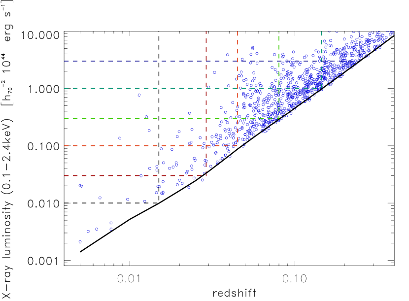
Figure 2: Median lower detection limit for the X-ray luminosity as a function of redshift in the flux-limited REFLEX II survey (black line). The data points show the luminosity and redshift distribution of the individual REFLEX II clusters. We also show the limits of six volume-limited subsamples of the REFLEX II survey used to assess the density distribution in this paper.

4 Results

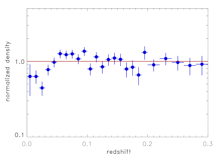
Figure 3: Cluster density distribution as a function of redshift for the REFLEX II galaxy clusters for a minimum luminosity of $10^{42}$ erg s^-1 (0.1 - 2.4 keV). The density distribution has been normalised by the predicted redshift distribution as explained in the text.

In Fig. 3 we show the density ratio distribution of the clusters for the entire REFLEX II cluster sample with $L_{x}\geq 10^{42}$ erg s^-1 out to a redshift of $z=0.3$. It was constructed by dividing the observed number of REFLEX II clusters in different redshift bins by the prediction based on the best fitting Schechter and REFLEX II selection function. 203 clusters are involved in tracing the density at $z\leq 0.06$ and 416 in the region out to $z=0.1$. While the overall cluster distribution is remarkably homogeneous, we note an underdensity of about 30 - 40% at $z\leq 0.04$ followed by an overdensity from $z=0.04$ to $z=0.07$.

To illustrate the point made above, that the determined density ratio distribution depends, to some extent, on the luminosity function adopted, we show in Fig. 4 the density ratio distributions for the three different luminosity functions listed in Table 1. For the X-ray luminosity function that is biased low at the low luminosity end, the underdensity effect weakens, as expected, but the overdensity in the redshift range $z=0.04-0.07$ becomes slightly more pronounced. However, there is still a significant density difference between the low density and higher density regions at low redshifts. For the function with a large bias at the low luminosity end the depth of the local underdensity increases.

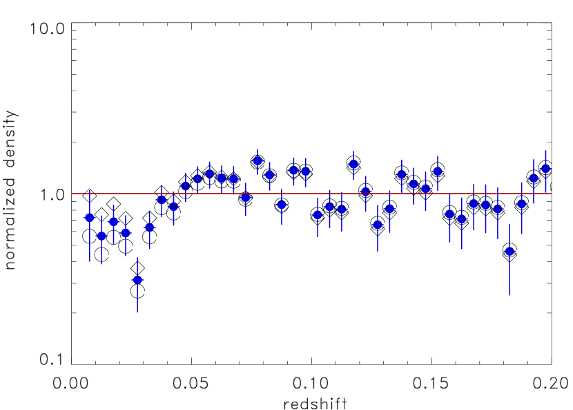
Figure 4: Cluster density distribution as a function of redshift for the REFLEX II galaxy clusters for a minimum luminosity of $10^{42}$ erg s^-1 (0.1 - 2.4 keV). Same as Fig. 3, adding the results for using the bracketing X-ray luminosity functions: low bias (open diamonds) and high bias (open circles).

To further test the robustness of the underdensity, we use a larger value of the lower X-ray luminosity limit of the sample. We show in Fig. 5 the density ratio distribution for a lower luminosity limit of $0.2\times 10^{44}$ erg s^-1 for which the cluster sample is volume-limited up to a redshift of $z=0.068$. We clearly detect the previously identified underdense and overdense regions within the range where the sample is volume-limited.

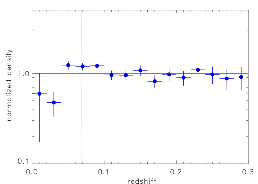
Figure 5: Cluster density distribution as a function of redshift for the REFLEX II galaxy clusters for a minimum luminosity of $0.2\times 10^{44}$ erg s^-1 (0.1 - 2.4 keV). The density distribution has been normalised by the predicted redshift distribution as explained in the text. The vertical dotted line shows the redshift range up to which the sample is essentially volume-limited.

Table 2: Comparison of the ratio of the observed to predicted cumulative number of clusters as a function of the redshift limit for the REFLEX II clusters sample. We also give the statistical uncertainty in brackets. The columns labeled (1) to (3) give the ratio of observed to predicted numbers for the REFLEX II sample for a lower X-ray luminosity limit of $L_{X}=10^{42}$ erg s^-1, for the best fitting, low, and high X-ray luminosity function. The last column, (4), shows the results for the REFLEX II sample with an X-ray luminosity limit of $L_{X}=0.2\times 10^{44}$ erg s^-1.

$$\begin{array}[]{lllll}\hline\cr\vskip 3.0pt plus 1.0pt minus 1.0pt\cr{\rm z\leavevmode\nobreak\ limit}&{\rm(1)}&{\rm(2)}&{\rm(3)}&{\rm(4)}\\ \vskip 3.0pt plus 1.0pt minus 1.0pt\cr\hline\cr\vskip 3.0pt plus 1.0pt minus 1.0pt\cr 0.02&0.63(\pm 0.11)&0.82(\pm 0.15)&0.50(\pm 0.09)&0.59(\pm 0.42)\\ 0.03&0.53(\pm 0.07)&0.67(\pm 0.09)&0.44(\pm 0.06)&0.27(\pm 0.15)\\ 0.04&0.61(\pm 0.07)&0.73(\pm 0.08)&0.52(\pm 0.05)&0.49(\pm 0.14)\\ 0.05&0.71(\pm 0.06)&0.83(\pm 0.07)&0.61(\pm 0.05)&0.76(\pm 0.12)\\ 0.06&0.81(\pm 0.05)&0.93(\pm 0.07)&0.72(\pm 0.05)&1.01(\pm 0.10)\\ 0.07&0.88(\pm 0.06)&0.98(\pm 0.06)&0.78(\pm 0.05)&1.05(\pm 0.09)\\ 0.08&0.93(\pm 0.05)&1.02(\pm 0.06)&0.84(\pm 0.05)&1.10(\pm 0.08)\\ \vskip 3.0pt plus 1.0pt minus 1.0pt\cr\hline\cr\vskip 3.0pt plus 1.0pt minus 1.0pt\cr\end{array}$$

Taking this approach one step further we show in Fig. 6 the density distribution traced by six different volume-limited subsamples obtained from REFLEX II. The luminosity and redshift boundaries for the samples are shown in Fig. 2. The colors of the subsample limits (in the electronic version of the paper) are the same as the colors of the data points in Fig. 6. The relative normalisations of the samples are based on weights determined from an integration of the observed interval of the X-ray luminosity function. These weights are given by

$$W_{i}={\int_{L_{X_{0}}}^{\infty}\phi(L)dL\over\int_{L_{X_{i}}}^{\infty}\phi(L)dL}\leavevmode\nobreak\ \leavevmode\nobreak\ \leavevmode\nobreak\ ,$$ (2)

where $L_{X_{0}}$ is a reference lower limit and $L_{X_{i}}$ is the lower X-ray luminosity limit of the sample. The reasonable agreement of the sample densities in the overlapping redshift regions provides a direct test of the quality of this inter-calibration. The different samples clearly trace the local underdensity and the following overdense region. Given the various tests presented, we can be confident that these density variations are real and not an artifact of the adopted luminosity function.

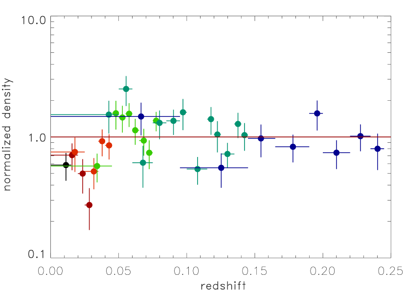
Figure 6: Relative density distribution of the REFLEX II clusters represented by six volume-limited subsamples as a function of redshift. The relative normalisation of the subsamples has been determined from Eq. 1 as explained in the text.

From an inspection of Table 2 we conclude on the following results. In the redshift range $z=0$ to $0.03$ we find an underdensity in the southern cluster distribution of about 40 - 50%. Taking the systematics of the luminosity function uncertainties into account, the statistical errors leave us with a detection confidence limit of $3.7\sigma$ for the $L_{X}\geq 10^{42}$ erg s^-1 sample and a significance larger than $4\sigma$ for the volume-limited sample shown in Fig. 5. For the redshift range $z=0-0.04$ we obtain an underdensity of about 30 - 40% with a significance of $3.4\sigma$ for the flux-limited sample and $3.6\sigma$ for the volume-limited sample.

These results are consistent with our previous findings from REFLEX I for an underdensity in the cluster distribution at $z<0.04$ and an overdensity in the region $z=0.05$ to $0.06$ (Schuecker et al. 2001). At a closer look, the REFLEX I results show no underdensity at $z<0.02$ and the overall deficit is slightly less pronounced. This is partly due to the fact that the low luminosity end of the REFLEX I X-ray luminosity function is less well sampled yielding a slightly smaller negative slope than for REFLEX II. With the new data, the X-ray luminosity function is better established leading to a better assessment of the low redshift density distribution.

To explore where the underdensity is located in the southern sky we study the sky distribution of all clusters at redshift $z\leq 0.06$. To correct for the different depth to which the luminosity function is probed at different redshifts and sky positions, we weight each cluster by the values determined by Eq. 2, where $L_{X_{i}}$ is the X-ray luminosity of the detection limit at the sky and redshift location of the clusters to be weighted. To limit the Poisson noise of the cluster distribution to a value significantly smaller than the actual density variations we smooth the sky distribution with a Gaussian kernel with a $\sigma$ of 10 degrees on the sky.

The resulting large-scale density distribution is shown in Fig. 7. We observe three prominent regions with overdensities by about a factor of two. The region around RA $=200^{o}$ and DEC $=-30^{o}$ is dominated by the Shapley supercluster. The region around RA $=300^{o}$ and DEC $=-55^{o}$ is marked by the supercluster 120 and the region RA $=50-100^{o}$ and DEC $=-55^{o}$ is marked by superclusters 42 and 62 identified in the REFLEX II sample by Chon et al. (2013). These superclusters are all located between $z=0.04$ and 0.065 and thus are mainly responsible for the overdensity in the total REFLEX II sample in this redshift range as found above. In particular the regions in the SGC at low declination and near the South Galactic Pole are mostly underdense.

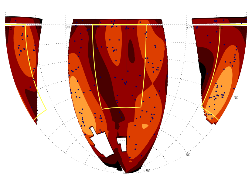
Figure 7: Cluster density distribution of REFLEX II galaxy clusters in the redshift shell z = 0.0 - 0.06 shown in equatorial coordinates. The density distribution was smoothed by a Gaussian kernel with $\sigma=10$ deg., normalised to an integral of 1. The color scale for the density ratio compared to the mean is defined by orange $\geq 2$, light red $=1-2$, brown $=0.5-1$, dark brown $\leq 0.5$. The regions of the Magellanic Clouds are excised from the REFLEX II Survey and the galaxy survey regions of Whitbourn & Shanks (2014) are indicated by yellow solid lines.

5 Comparison to galaxy redshift surveys

We can compare our results in more detail with the findings from galaxy redshift surveys of a local underdensity. We use the galaxy cluster distribution to specifically investigate two of the sky regions studied by Whitbourn & Shanks (2014) in the southern sky by means of the 2MASS photometric and 2MASS and 6dF redhift surveys. The regions are located in the SGC (6dF SGC, 3511 deg²) at RA $=0-50^{o}$ and $330-360^{o}$ ) with DEC $=-40-0^{o}$ as well as at RA $=150-220^{o}$ with DEC $=-50-0^{o}$ in the NGC (6dF NGC, 2578 deg²) . We extract cluster data from exactly the same regions as indicated in Fig. 7. In Figs. 8 and 9 we show the relative redshift distribution of the REFLEX II clusters in these areas. The distribution functions shown are again the ratio of the observed to predicted galaxy clusters for the best fitting X-ray luminosity function. We note the underdensity in the redshift region $z=0$ to $0.05$ (corresponding to $\sim 212$ Mpc) in the SGC region, while the NGC shows no such significant underdensity. The plots also show the density distributions determined by Whitbourn & Shanks (2014) for the 6dF-SGC and 6df-NGC regions as a function of redshift out to $z=0.1$. The correspondence of the galaxy and cluster distributions are suprisingly close. Peaks and troughs are traced by both distribtions in almost the same way.

A comparison of our galaxy cluster distribution with the results of Keenan et al. (2013) is more difficult, since their survey only covers a total area of $\sim 585.4$ deg² with three different subregions of which two overlap with the REFLEX survey. These two regions cover a band with a width of $\pm 2$ degrees around the equator. The region in the SGC stretches roughly from RA of 300 to 80 degrees and the one in the NGC from about RA of 130 to 260 degrees. Since this sky area is much smaller than that of the former study, the cluster number statistics is too poor to precisely trace the density distribution. To improve the statistics at least by some factors, we look at the cluster distribution in a latitude band in the declination range -4^o to +2.5^o. In the entire region in this declination range covered by REFLEX we cannot detect any significant depression in the density distribution at low redshift. If we, however, limit our study to the right ascension region of the SGC given above, we find an underdensity in the redshift range $z=0.0$ to $0.075$ and a peak at $z=0.08$ to $0.1$. This is similar to the observations of Keenan et al. for the SGC. The density peak at $z\sim 0.09$ is connected to the region containing the Sloan Great Wall. For the NGC region we do not observe a low density at low redshift, but an indication for underdense regions at $z=0.04$ to $0.05$ and at $z=0.06$ to $0.08$. Thus there is some similarity of the results. But the comparison is based on small number statistics for the clusters and we cannot expect a precise correspondence.

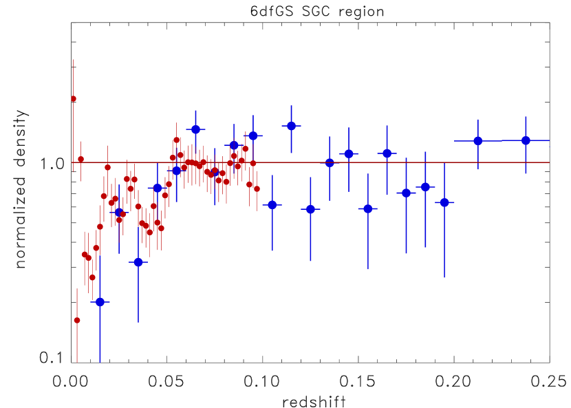
Figure 8: REFLEX II cluster density distribution as a function of redshift for the region RA $=0-50,330-360^{o}$ and DEC $=-40-0^{o}$ in the south galactic cap for a minimum luminosity of $0.2\times 10^{44}$ erg s^-1 (0.1 - 2.4 keV). The density distribution has been corrected by means of the survey selection function and normalised to unity. The region corresponds to region 6dFGS-SGC of Whitbourn & Shanks (2014). We also show the results of their assessment of the galaxy distribution out to $z=0.1$ in this region with small red data points.

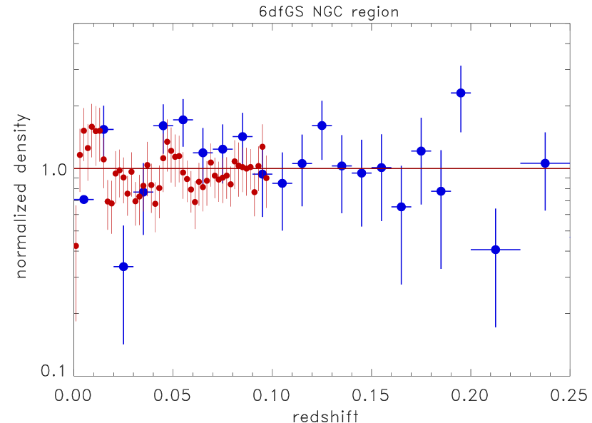
Figure 9: REFLEX II cluster density distribution as a function of redshift for the region RA $=150-220^{o}$ and DEC $=-50-0^{o}$ in the north galactic cap for the same luminosity limit as in Fig. 8. The density distribution has been corrected by means of the survey selection function and normalised to unity. The region corresponds to region 6dFGS-NGC of Whitbourn & Shanks (2014). We also show the results of their assessment of the galaxy distribution out to $z=0.1$ in this region with small red data points.

Table 3: Comparison of the ratio of the observed to predicted cumulative number of clusters as a function of the redshift limit for the REFLEX II clusters in the 6dFGS-SGC and 6dFGS-NGC regions. We also give the statistical uncertainty in brackets.

$$\begin{array}[]{lll}\hline\cr\vskip 3.0pt plus 1.0pt minus 1.0pt\cr{\rm z\leavevmode\nobreak\ limit}&{\rm SGC}&{\rm NGC}\\ \vskip 3.0pt plus 1.0pt minus 1.0pt\cr\hline\cr\vskip 3.0pt plus 1.0pt minus 1.0pt\cr 0.02&0.17(\pm 0.12)&1.41(\pm 0.41)\\ 0.03&0.37(\pm 0.12)&0.86(\pm 0.22)\\ 0.04&0.35(\pm 0.10)&0.83(\pm 0.18)\\ 0.05&0.45(\pm 0.10)&1.02(\pm 0.17)\\ 0.06&0.54(\pm 0.09)&1.15(\pm 0.16)\\ 0.07&0.69(\pm 0.10)&1.16(\pm 0.15)\\ 0.08&0.72(\pm 0.09)&1.17(\pm 0.14)\\ 0.10&0.84(\pm 0.09)&1.18(\pm 0.12)\\ \vskip 3.0pt plus 1.0pt minus 1.0pt\cr\hline\cr\vskip 3.0pt plus 1.0pt minus 1.0pt\cr\end{array}$$

6 Discussion

As discussed in the literature described above, an underdense region may become cosmologically interesting in terms of mimicking the observed accelerated expansion if the underdense region has a minimum size of $\sim 300$ Mpc and if our location is within 10% of the center of the void (e.g. Alexander et al. 2009). A first inspection of the redshift distribution of the REFLEX clusters indicates that the cluster density is on average underdense in the REFLEX region at $z\leq 0.04$ which corresponds to a comoving radius of only $\sim 170$ Mpc. Thus the detected underdensity is significantly smaller than what is required for the above void models. Several tests showed that this underdensity is not an artifact of the X-ray luminosity function used for the analysis. The homogeneity of the density distribution on larger scales, as observed in the redshift range up to $0.3$ confirms that the observed density variations are confined to smaller volumes. This $z\leq 0.3$ survey region corresponds to a maximum distance of 1.19 Gpc and a survey volume of 2.4 Gpc³. In comparison, the size of the volume in which we observe the cluster distribution to be significantly underdense is 0.007 Gpc³. Thus the REFLEX survey shows an almost homogeneous Universe on scales larger than about 300 Mpc. This latter result supports the picture that the REFLEX II survey is large enough to constrain the extent of a local void.

In the next step of our analysis we probed the cluster distribution in more detail, and find that the underdensity in the local southern sky is mostly confined to the regions of the South Galactic Pole and the SGC at low galactic latitudes. The good correspondence of the galaxy and cluster distribution in the latter area and in the NGC region gives further support to the reliability of our measurements. These results also show, however, that we are not located in an isotropic underdense region. Therefore we conclude that the local large-scale structure traced by REFLEX II does not support a local large-scale void conforming to the minimum void models. Most of the works that claim a detection of a local void are dominated by galaxy data preferentially from regions in the SGC near the equator and near the South Galactic Pole (Huang et al. 1997, Frith et al. 2003, 2006, Busswell et al. 2004, Keenan et al. 2013, Whitbourn & Shanks 2014). These regions show local underdensities in our studies while other sky regions are not underdense at low redshifts.

For a more quantitative characterisation of the local underdensity we have to consider that galaxy clusters have a biased distribution with respect to the matter distribution. The biasing factor is a function of cluster mass and in a sample of clusters it depends on the biasing averaged over the mass distribution. For the REFLEX cluster sample the average bias has been modelled as a function of the lower luminosity limit (Balaguera-Antolinez et al. 2011, Chon et al. 2014). For the redshift range $z=0-0.04$ the lower luminosity limit varies from $L_{x}(min)=10^{42}$ erg s^-1 to $L_{x}(min)=6\times 10^{42}$ erg s^-1 and the biasing factor is in the range 2.5 to 3. The theoretical concept of cluster biasing has been verified with REFLEX with uncertainties smaller than the statistical uncertainties in the present study. Thus for an underdensity in the cluster distribution of about $40(\pm 15)\%$ we expect the matter distribution to have a smaller underdensity of about $15(\pm 5)\%$.

Also for a quantitative comparison to the galaxy distribution we have to take this bias into account, since galaxies are hardly biased. Table 3 lists the cumulative cluster density inside various redshifts normalised to the expectations for the 6dF-SGC and 6dF NGC region. We note that for $z\leq 0.04$ the cluster density is lower in the 6dF-SGC area by about $60(\pm 22)\%$ including systematic errors. This corresponds to an unbiased underdensity of about $22(\pm 8)\%$. The underdensity in the galaxy distribution as noted in Fig. 8 is about $40\%$, a bit higher than our prediction, but still in reasonable agreement given the large statistical uncertainties.

7 Summary and Conclusion

With the well understood selection function of the REFLEX II galaxy cluster sample, we can trace the large-scale density distribution over a large region in an unbiased way. Here we focussed on the study of the local density distribution in the southern sky.

We traced the cluster distribution in the extragalactic sky to a redshift of $z\sim 0.3$, corresponding to a comoving distance of $\sim 1.2$ Gpc and a survey volume of 2.4 Gpc³, and find the cluster distribution remarkably homogeneous on large scales. With this result we can establish a large scale mean cluster density, which allows us a precise assessment of more local density variations and to confine their extent well within our survey volume.

For the redshift range $z=0$ to $0.04$ we find the cluster density to be lower than the large-scale average by about 30 - 40% with a significance larger than 3.4 $\sigma$. With the expected bias of the cluster density variations compared to those of the dark matter, we infer an average dark matter underdensity of about $15(\pm 5)\%$ in the southern extragalactic sky. This underdensity translates into a locally larger Hubble constant of about $\sim 3(\pm 1)\%$ assuming $\Lambda$CDM cosmology.

A closer inspection shows that this is not an isotropic underdensity in the southern sky. A special region that contributes most to the observed underdensity is located in the South Galactic Cap within REFLEX II.

A comparison of the density distribution of galaxies and clusters in the South and North Galactic Cap in the southern sky with data coming from Whitbourn & Shanks (2014) and from our REFLEX survey shows that both object populations trace the same density distribution. In both surveys that SGC shows an underdensity at redhifts from $z=0$ to $0.05$ and no local underdensity in the NGC.

Observations of a local underdensity in the galaxy distribution on scales up to 300 Mpc have given rise to intense speculations that the cosmic acceleration deduced from the observations of SN type Ia can be explained by a local void region. Our results show that the local underdensity is significantly smaller than required by minimum void models and a locally underdense region is not observed in all directions in the southern sky.