Coronal Fourier power spectra: implications for coronal seismology and coronal heating

Abstract

The dynamics of regions of the solar corona are investigated using Atmospheric Imaging Assembly (AIA) 171Å and 193Å data. The coronal emission from the quiet Sun, coronal loop footprints, coronal moss, and from above a sunspot is studied. It is shown that the mean Fourier power spectra in these regions can be described by a power-law at lower frequencies that tails to flat spectrum at higher frequencies, plus a Gaussian-shaped contribution that varies depending on the region studied. This Fourier spectral shape is in contrast to the commonly-held assumption that coronal time-series are well described by the sum of a long time-scale background trend plus Gaussian-distributed noise, with some specific locations also showing an oscillatory signal. The implications of this discovery to the field of coronal seismology and the automated detections of oscillations are discussed. The power-law contribution to the shape of the Fourier power spectrum is interpreted as being due to the summation of a distribution of exponentially decaying emission events along the line of sight. This is consistent with the idea that the solar atmosphere is heated everywhere by small energy deposition events.

1. Introduction

Coronal seismology is the study of oscillatory phenomena in the solar corona. First suggested by Uchida (1970), the practice of coronal seismology attempts to locate oscillatory phenomena in the solar corona, identify the wave modes present, and then use theoretical descriptions of those wave modes to infer the physical conditions of the solar corona. The practical application of coronal seismological ideas began in earnest with observations of wave modes described in DeForest & Gurman (1998) and Berghmans & Clette (1999) from data captured by Extreme Ultraviolet Telescope (EIT, Delaboudinière et al., 1995) on board the Solar and Heliospheric Observatory (SOHO, Domingo et al., 1995), and also by (Aschwanden et al., 1999) using data from the Transition Region and Coronal Explorer (TRACE, Handy et al., 1999). Since these initial works, many papers have been published describing oscillatory phenomena in the corona and their interpretation in terms of theoretically known wave modes. The review articles Nakariakov & Verwichte (2005) and De Moortel & Nakariakov (2012) refer to many more articles on both observational and theoretical coronal seismology.

Oscillatory phenomena in the solar corona are relatively rare, both spatially and temporally. Two types of oscillatory motions have received a lot of attention. The first is known as a transverse oscillation, since the loop motion is approximately transverse to the extent of the loop (Nakariakov et al., 1999). These motions appear to be triggered by nearby flaring events, and are identified with the fundamental harmonic of the kink mode of the flux tube that comprises the coronal loop. The second type is known as a longitudinal oscillation, or propagating disturbance (PD). These waves propagate along flux tubes, and have been identified as slow mode magnetohydrodynamic (MHD) magneto-acoustic waves (although alternative interpretations do exist that do not invoke oscillatory phenomena, for example, Pontieu & McIntosh, 2010 and Tian, McIntosh, & Pontieu, 2011).

Other types of oscillatory behavior have been observed. McAteer et al. (2005) demonstrate the presence of oscillatory power with periods in the range of 40-80 seconds using high-cadence H$\alpha$ blue wing observations of a Geostationary Operational Environmental Satellite (GOES) C9.6-class solar flare obtained at Big Bear Solar Observatory using the Rapid Dual Imager (Phillips et al., 2000; Jess et al., 2007). The measured properties of these oscillations are consistent with the existence of flare-induced acoustic waves within the overlying loops. In addition, An$\bar{\mbox{d}}$ić & McAteer (2013) show that the oscillatory power in the lower solar atmosphere of active regions increases in response to flare events at distant solar locations.

The relative scarcity of observations of coronal oscillations has prompted efforts to create automated oscillation detection algorithms. The need for an automated oscillation detection algorithm has been exacerbated by the large and rapidly growing amount of Solar Dynamics Observatory (SDO, Pesnell et al., 2012) Atmospheric Imaging Assembly (AIA, Lemen et al., 2012) data. There have been several attempts at designing such algorithms. De Moortel & McAteer (2004) describe the design of an automated oscillation-detection algorithm based on wavelet analysis. The algorithm finds significant wave packets ranging from single to multiple wave cycles in duration, by a wavelet power/confidence level comparison against the null hypothesis that a given time series is Gaussian-distributed noise. Pixels with significant oscillatory content are grouped manually. Nakariakov & King (2007) take a similar approach, using a thresholded fast Fourier transform to find locations in TRACE data that may support an oscillatory signal. The threshold level is defined as three to four times the average fast Fourier transform (FFT) power; if the maximum FFT power is above this level then the frequency at which that power occurs is assumed to be real. Ireland et al. (2010) assume that an oscillatory signal is present in each location in the datacube and then use a Bayesian-based treatment to calculate the probability that the frequency has a particular value. This algorithm relies on subtracting a background trend from the time-series being tested, and assumes that the noise is Gaussian distributed.

The above algorithms precipitate detections based on the strength of the signal of an oscillation on a pixel by pixel basis, and then group these pixels together using some set of criteria. The automated detection algorithm of Sych & Nakariakov (2008) begins by identifying candidate oscillatory regions as those whose time-series of emission show a high variance (Grechnev, 2003) (under the implicit assumption that the time-series has an approximately constant mean value). Detections are based on wavelet filtering of these regions in all three dimensions of the data cube simultaneously, with the implicit assumption that the noise is Gaussian-distributed. The algorithm of McIntosh et al. (2008) differs from the previous algorithms: it begins by Fourier transforming the entire data cube, and calculating the coherence of neighboring pixels in narrow frequency bands, and filtering the results. The null hypothesis here is that pairs of time series that have low coherence can be rejected as being part of an oscillatory group. This method uses a symmetric filter to estimate the coherence, in that oscillatory power from either side of the central search frequency contributes the same weight to the final result. There is an implicit assumption here that the power on either side of the central search frequency is approximately the same. In this algorithm, the spatial extent of the coherence of the oscillatory signal is the key identifier of a wave process.

All these detections algorithms, and many detections in the literature make either the explicit or implicit assumption that the observed time-series consists of a background trend of some kind and (approximately) Gaussian-distributed noise which must be taken in to account in order to test for the presence of an oscillatiory signal (De Moortel & McAteer, 2004; Nakariakov & King, 2007; Sych & Nakariakov, 2008; Ireland et al., 2010; Calabro et al., 2013). However, two recent papers cast doubt on this assumption. Auchère et al. (2014) integrate emission over small portions of active regions and the quiet Sun as observed in the 195Å passband images from EIT and show that the resulting time-series has an approximate power-law Fourier power spectrum over the frequency range 0.01 - 1 mHz. Gupta (2014) showed power-law power spectra in the intensity at six single points in AIA 171Å coronal plumes extending over the frequency range $0.3\rightarrow 4.0$ mHz.

The aim of this paper is to investigate the nature of the Fourier power spectrum in regions of interest to coronal seismology, to look for evidence that the above assumption is appropriate. The nature of coronal emission has implications for coronal seismology, and may be indicative of the nature of the fundamental energy deposition that keeps the corona hot. Section 2 describes the observations used, while Section 3 describes the method of analysis employed and presents the results. Section 4 discusses the implication of these results for coronal seismology and the heating of the solar atmosphere. Section 5 summarizes the discussion and outlines future work.

2. Observations

AIA observes images of the Sun in multiple wavebands simultaneously and continuously, at high cadence (12 seconds) and at high spatial resolution (0.6 arcseconds per pixel). These data enable detailed comparisons between phenomena observed in multiple wavebands, and are therefore ideal for assessing the frequency content of the solar atmosphere. AIA data was acquired using the Lockheed Martin Solar Astrophysics cutout service at http://lmsal.com/get_aia_data/. Six hours of image data in the time range 2012-09-23 00:00 - 06:00 UT, at the full 12 second cadence, in the 171Å and 193Å wavebands is used. These wavebands were selected because previous studies in similar wavebands (TRACE 171Å and 193Å) show the presence of coronal oscillations. The selected area covers a single $\beta\gamma$ active region, NOAA AR 11575. This area was selected for two reasons. First, it is quiescent in that there were no X-ray flares or other large-scale disturbances (for example, filament eruptions or rearrangments of long bright coronal loops) over the spatial extent of the cutout within the time range (Figure 1). Therefore, any variations in the plasma properties cannot be ascribed to large-scale disturbances. Second, the selected cutout region contains a sunspot, and sunspots are known to be locations over which three minute oscillations have been detected by other instruments (De Moortel et al., 2002).

The data was prepared for analysis using the SolarSoft / IDL routines READ_SDO and AIA_PREP. These procedures convert the downloaded level 1.0 FITS cutout files to level 1.5 FITS files. This involves translating, scaling and rotating the images so they have the same sun-center, image scale with solar north in the same direction. All further processing from this point was performed in the SunPy 0.4 (http://www.sunpy.org) data analysis environment. Images were de-rotated to compensate for solar rotation, based on the center of the field of view of each image. After de-rotation, each image layer was coaligned with a reference layer, defined to be half way through the dataset, in this case at approximately 03:00 UT (Figure 1). This process is required since the solar de-rotation function used does not fully compensate for all the solar rotation. Coalignment was implemented using a template matching technique (Lewis, 1995) implemented by the scikit-image (van der Walt et al., 2014) routine match_template. A rectangular template sub-image with sides one half the size (in pixels) of the reference layer is defined. The coalignment algorithm finds the location of the best match of this template with each layer. The image layer is then shifted (using sub-pixel shifts) according to the location of the best match of the template with the image. This process removes residual bulk motions of the images.

3. Analysis

We wish to analyze the frequency content of these resulting datacubes as a function of spatial location. Four locations were chosen in the data representing four different types of physical locations in the solar atmosphere. These were a quiet Sun region, a region that lies on top of a sunspot, a footpoint region, and a coronal moss region. Figure 1 shows the location of the regions on sample images from the time range considered. These locations, selected by visual inspection, were chosen because they are representative of commonly observed structures in the corona. Further, oscillatory power has been identified previously over sunspots and loop footpoints (De Moortel et al., 2002) and moss structures (De Pontieu et al., 2003). A quiet Sun region is also included for comparison.

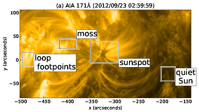
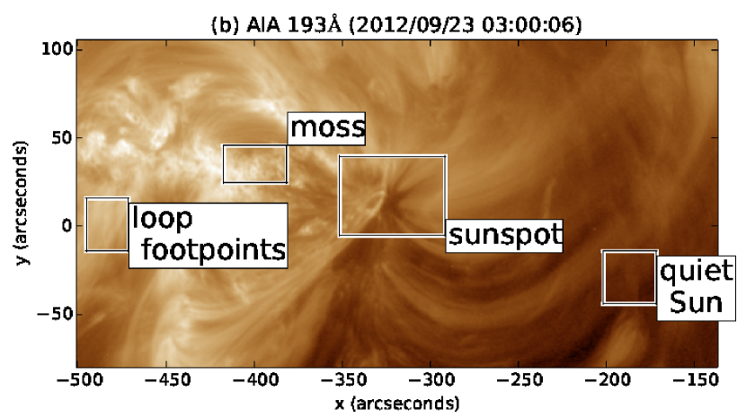
Figure 1.— Locations of the regions analyzed in each of AIA 171Å and 193Å, overlaid on sample images taken halfway through the six hour span used to form the time-series analyzed. The spatial extent of the data is (-501”, -138”) in the x-direction, and (-80”, 107”) in the y-direction, in heliocentric cartesian co-ordinates. The images show NOAA AR 11575 and some surrounding area.

Consider the emission from a single pixel, $I(t)$. The Fourier power spectrum for this emission was calculated as follows. First, the time-series was normalized by calculating $(I(t)-\langle I(t)\rangle)/\langle I(t)\rangle$. Secondly, the normalized time-series was apodized using the Hanning window, reducing ringing effects in the power spectrum. The full 12 second cadence is used, yielding time series of 1800 samples. The full spatial resolution is also retained in order to obtain fine detail on the variation of frequency content as a function of location. Figure 2 show example power spectra, plotted using a log-log scale, from a single location inside each of the regions shown in Figure 1. The shape of the power spectra indicate that the Fourier power approximately follows a power-law at lower frequencies, and flattens out at higher frequencies.

There is evidence that these power-laws extend to much longer frequencies than those considered here, down to approximately 0.01 mHz. Auchère et al. (2014) integrate emission over small portions of active regions and the quiet Sun as observed in the 195Å passband images from EIT and show that the resulting time-series has an approximate power-law Fourier power spectrum over the frequency range 0.01 - 1 mHz.

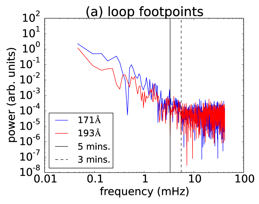
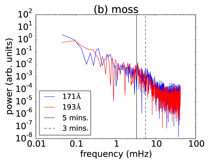
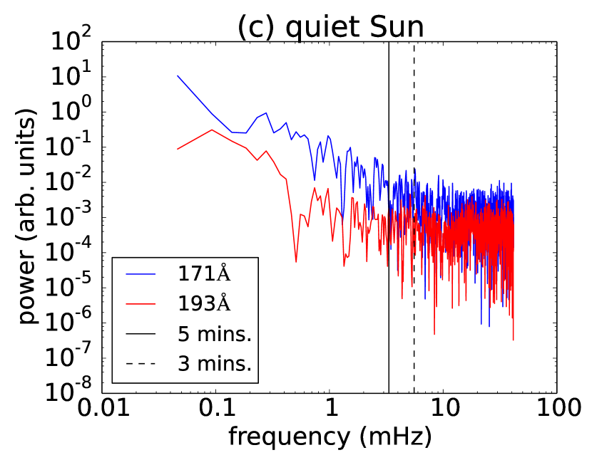
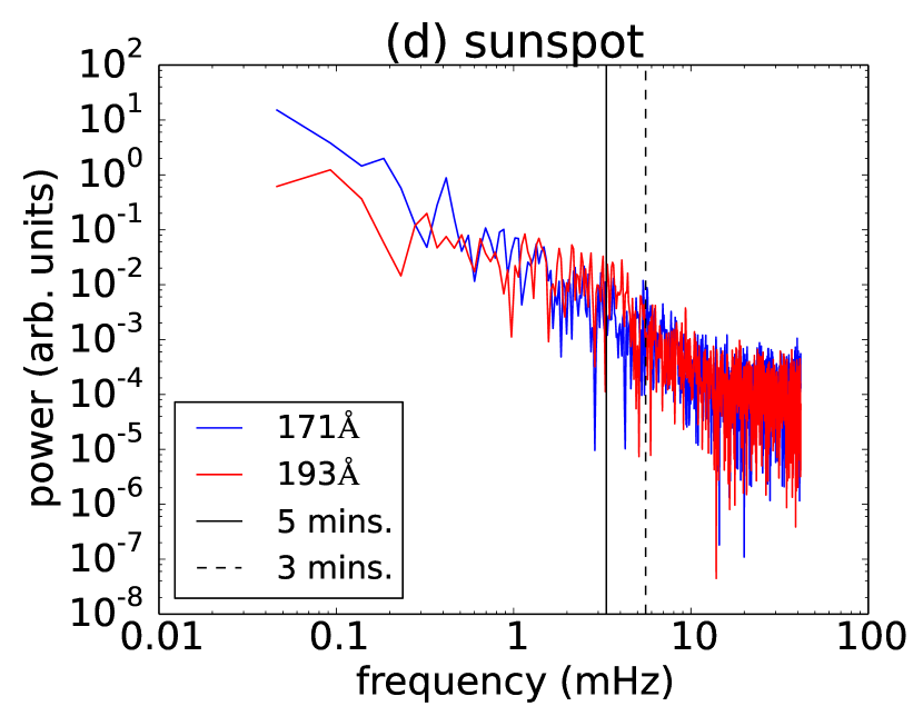
Figure 2.— Log-log plot of the Fourier power of a time-series at the AIA pixel overlying a randomly chosen pixel in each of the regions considered (see Figure 1). The vertical black lines indicate the 3 and 5 minute frequencies.

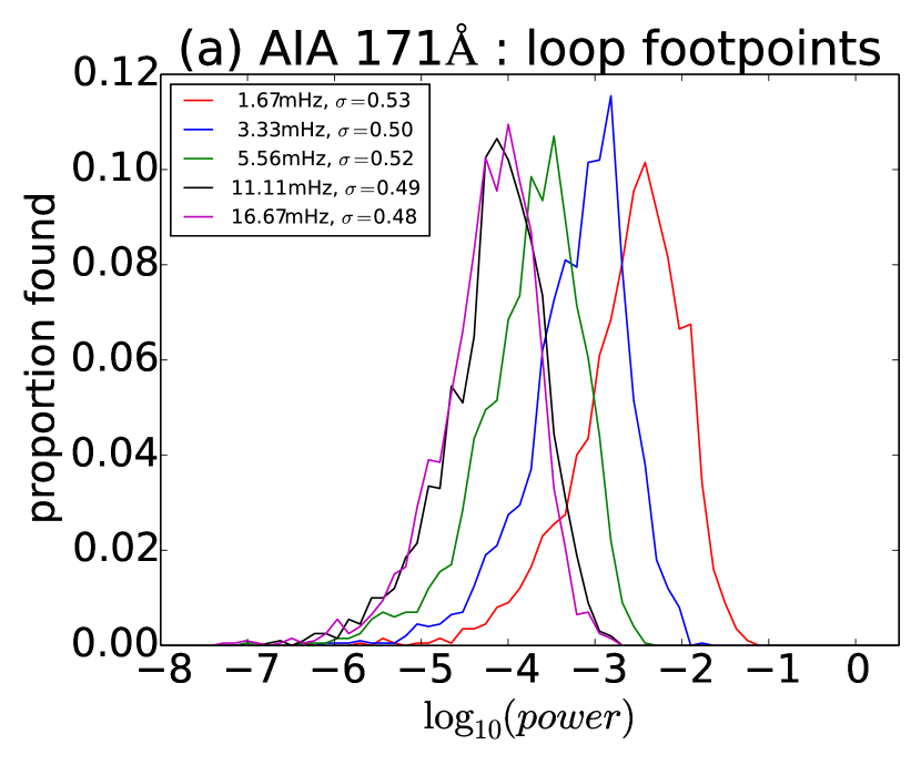
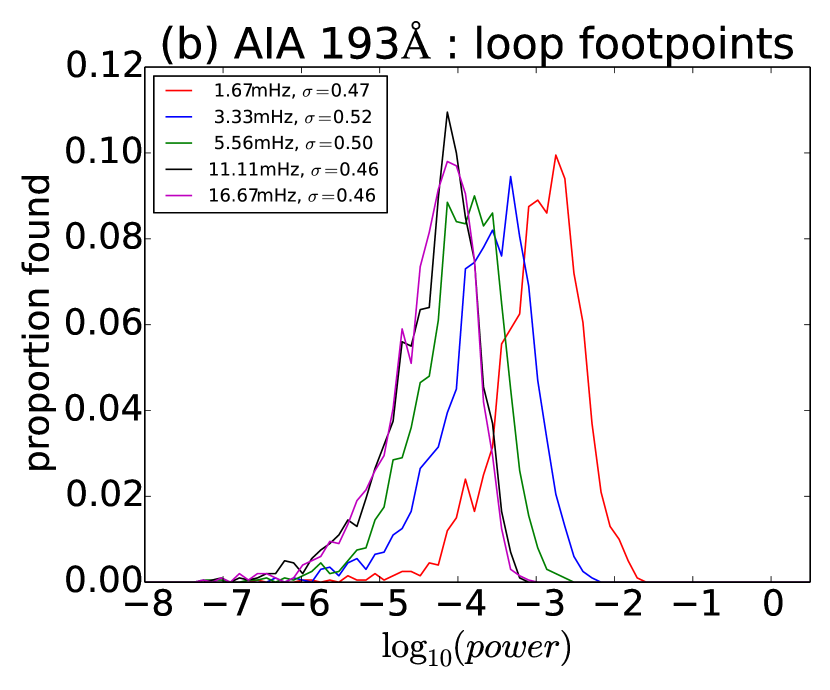
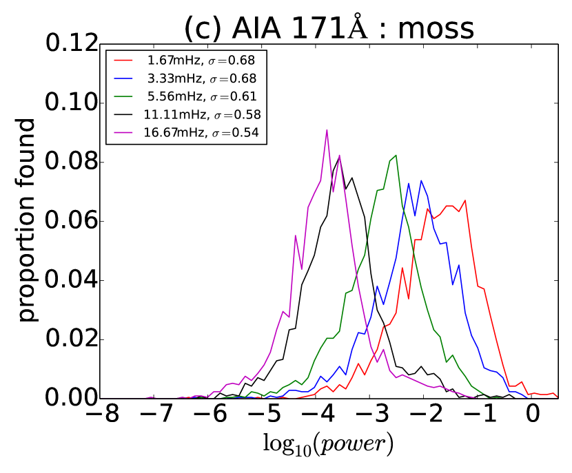
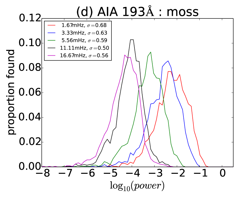
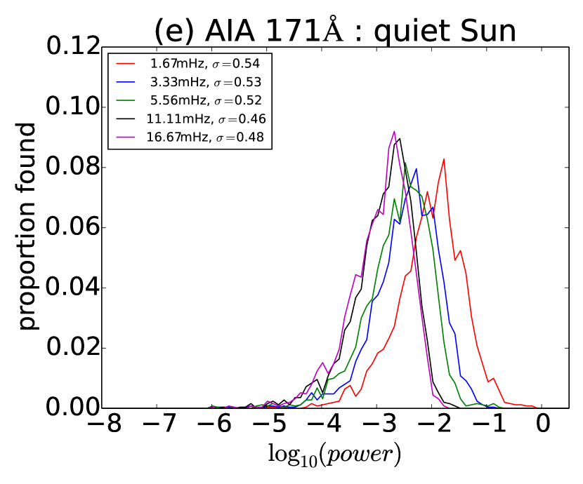
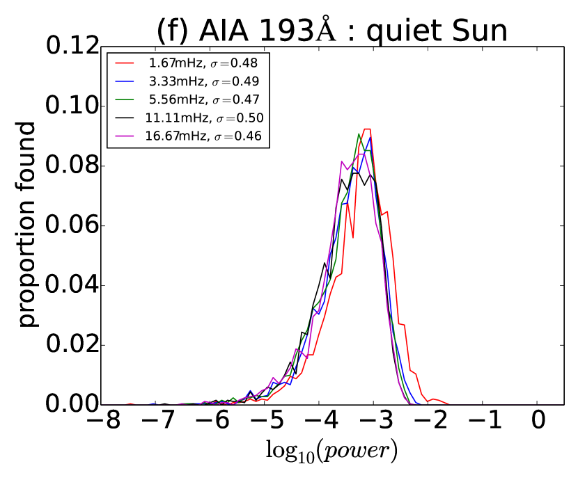
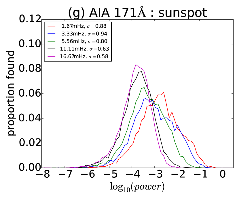
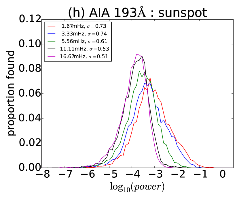
Figure 3.— The proportion of the number of pixels in each image that have a given Fourier power at some sample Fourier frequencies. The left hand column gives results for AIA 171Å, and the right hand column, AIA 193Å. Regions are indicated in each plot title.

Figure 3 shows the probability distribution of the Fourier power of the pixels in each region at five selected frequencies, for all the pixels in each region. These distributions are centrally peaked, show a slightly heavier tail towards lower Fourier powers (negative skew), are slightly broader when compared to a Gaussian distribution, and are all unimodal. These observations guide the choice of how to average the power spectrum over each of the selected region. The nature of these distributions suggest that the arithmetic mean of the Fourier power is biased by the very largest powers. Therefore, the mean value of the logarithm of the Fourier power is a better description of the range of values in the data (this is equivalent to the geometric mean of the Fourier power). The power spectra used below are calculated from the mean value of the logarithm of the Fourier power.

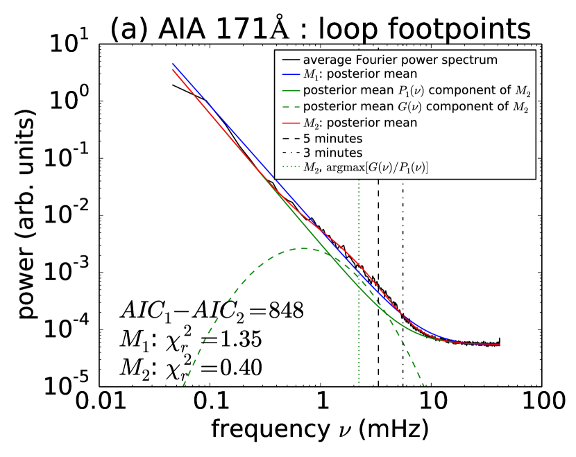
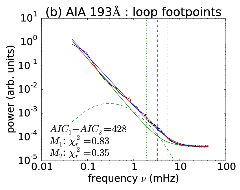
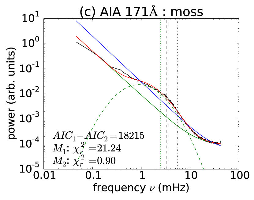
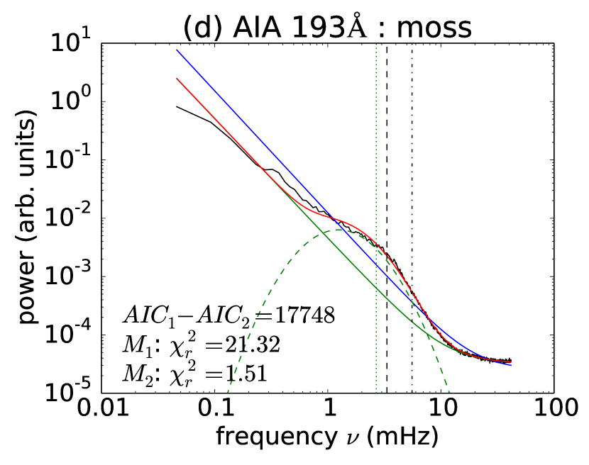
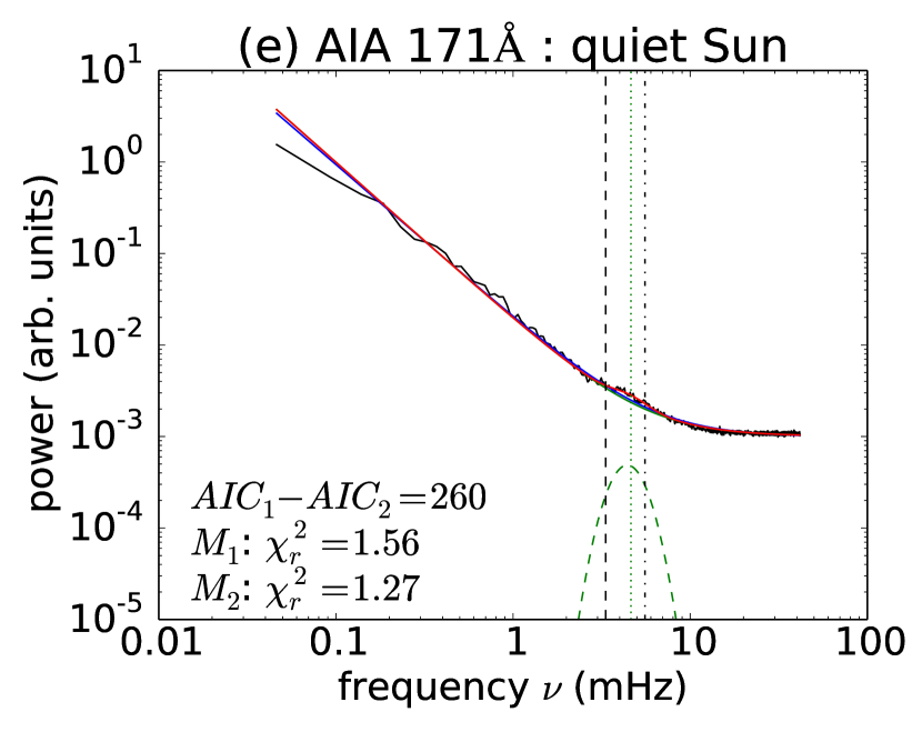
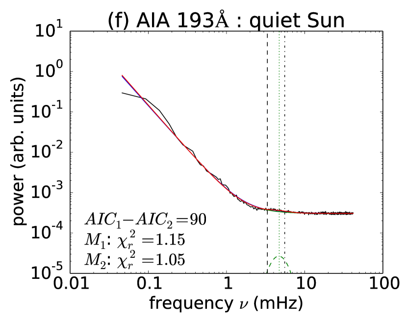
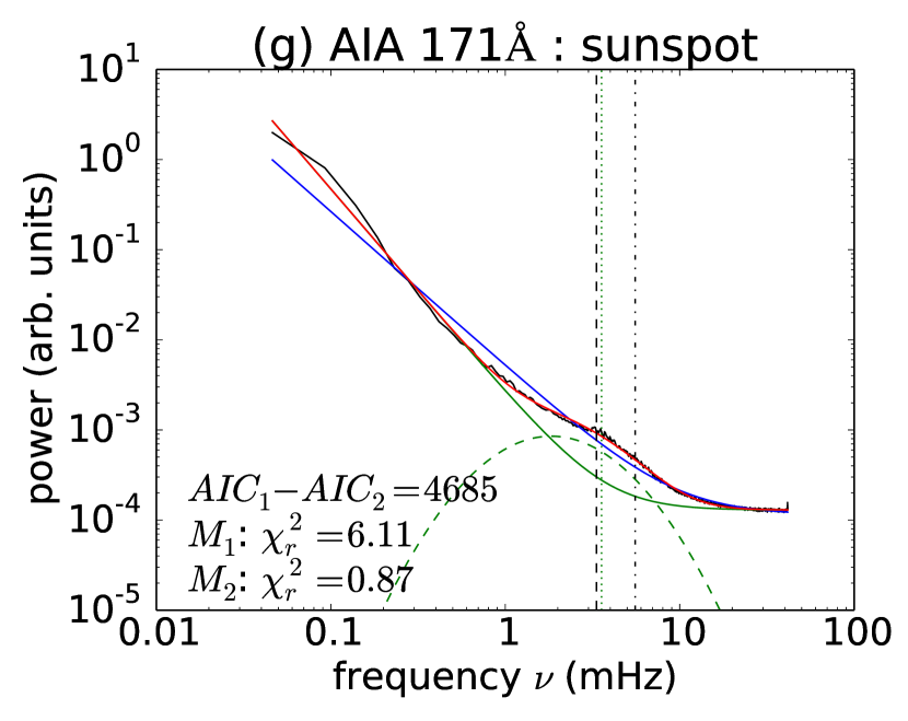
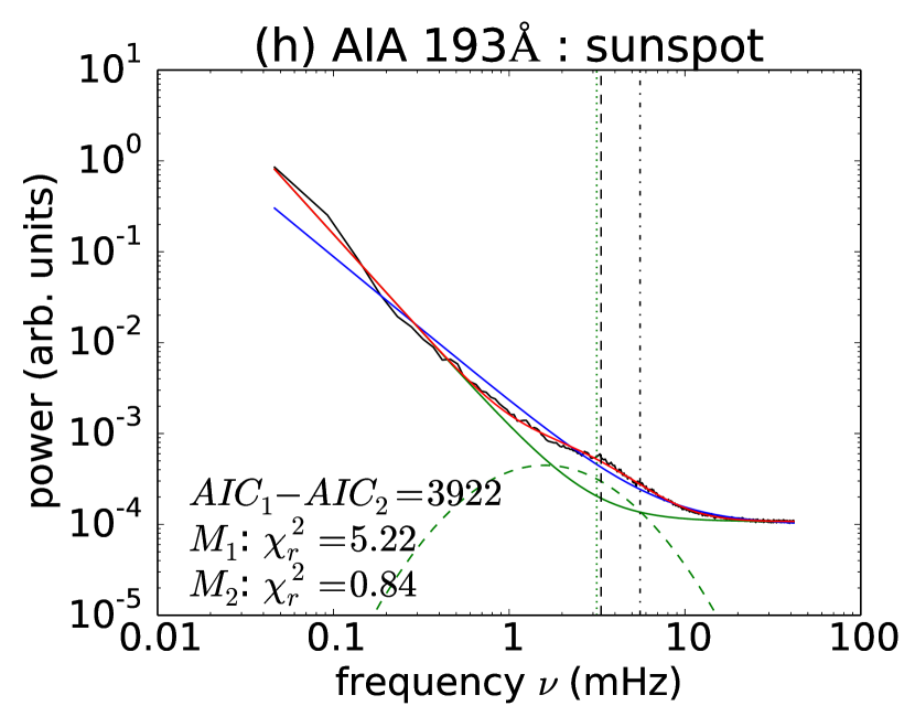
Figure 4.— Geometric mean of the Fourier power spectra (black solid line) in each of the four regions studied in AIA 171Å (left column) and AIA 193Å (right column). Also shown are the posterior mean fits for model $M_{1}$ and $M_{2}$ (blue and red lines respectively; see Section 3 and Appendix A for more detail). The AIC describing the preference for model over the other is also indicated in each plot. The reduced $chi^{2}_{r}$ statistic for Model 1 and Model 2 are given. The two components to Model 2, $P_{1}(\nu)$ and $G(\nu)$ are also shown in green; the location of the maximum of the $G(\nu)/P_{1}(\nu)$ ratio is indicated by the green dotted line. Model fit parameter values and their 68% credible intervals are quoted in Table 1.

The (geometric) mean Fourier power spectra are shown in Figure 4 for each of the physical regions considered. It is clear that, in general, the mean Fourier power spectra exhibit power-law like characteristics. The results for the quiet Sun, loop footpoints and sunspot regions suggest a power-law power spectrum. This can be modeled as

$$\mbox{Model $M_{1}$}:P_{1}(\nu)=A\nu^{-n}+C,$$ (1)

where $\nu$ is the frequency, $A>0$ is a proportionality constant and $n>0$ is the power-law index. The quantity $C>0$ models the high-frequency / low power end of the spectrum where the detection properties of the detector apparatus are assumed to dominate the observations.

The moss results for 171Å and 193Å are notably different from the other results. In comparison to the general trend observed in other regions, there appears to be excess Fourier power in the range 1-10 mHz. De Pontieu et al. (2003) show that TRACE 171Å time-series of bright upper transition region emission above active region plage (also known as moss) is a source of wavelet power. Periods of significant wavelet power are found in the range 200 to 600 seconds, and typically persist for 4–7 cycles. Later work by De Pontieu et al. (2005) suggested that spicule flux tubes tilted with respect to the solar surface provide a mechanism by which oscillatory power from lower in the atmosphere may be channeled to upper portions of the atmosphere. This suggests that a second model $M_{2}$ for the Fourier power spectrum in regions should be considered. The second model $M_{2}$ has two contributions to the overall Fourier power spectrum; a background power-law of the form of $P_{1}$, and a contribution that is more localized, $G(\nu)$. The model is given by

$$\mbox{Model $M_{2}$}:P_{2}(\nu)=P_{1}(\nu)+G(\nu)$$ (2)

where the localized contribution is described by

$$G(\nu)=\alpha\exp\left[-\frac{(\ln(\nu)-\beta)^{2}}{2\delta^{2}}\right].$$ (3)

Both these models are fit to the geometrically averaged Fourier power spectrum in both wavelengths and in all four regions (Figure 4). Model fitting and parameter estimation are implemented using a Bayesian probability based approach. This approach was chosen for its flexibility and consistent error estimation properties (Ireland et al., 2013). The details of the model fitting process are described in Appendix A. The position of $G(\nu)$ is restricted by permitting $\beta$ to vary in the range $0.1-10$ mHz only. This restriction, which is imposed in the fitting process (see Appendix A), arises from the observations of significant wavelet power in the period range 200 - 600 seconds as found by De Pontieu et al. (2003). After this fitting process is complete, the models are compared to decide which model best describes the data. The details of the model comparison process are described in the following section.

3.1. Results

Figure 4 show the fit results of each model to the data. For details on the fitting procedure, see Appendix A. The two models are assessed for how well they describe the data in two different ways. Model selection is implemented using the Akaike Information Criterion (AIC; Akaike, 1974). The AIC measures the amount of information lost when fitting a model to data (Takeuchi, 2000). The AIC is defined as

$$AIC\equiv 2k-2\ln L_{max}$$ (4)

where $L_{max}$ is the maximum likelihood achievable by the model, and $k$ is the number of parameters in the model ($k=3$ for Model 1, and $k=6$ for Model 2). Model selection is guided by calculating $\triangle AIC=AIC_{1}-AIC_{2}$. Positive values of $\triangle AIC$ indicate that Model 2 loses less information compared to Model 1, leading to a preference for Model 2 over Model 1 (Liddle, 2007). The AIC indicates that Model 2 is overwhelmingly preferred to Model 1 (see Figure 4). The AIC reveals which (out of a set of models) is preferred. It does not give an assessment of the goodness-of-fit of each model. Goodness-of-fit is estimated by calculating reduced-$\chi^{2}$, $\chi^{2}_{r}=\sum_{j=1}^{N}\left[(P_{i}(\nu_{j})-D_{j})/\sigma_{j}^{2}\right]/(N-k-1)$, where $N=899$ is the number of frequencies, $P_{i}(\nu_{j})$ is the model power $P_{i}$ at frequency $\nu_{j}$, $D_{j}$ is the mean Fourier power spectra at $\nu_{j}$, and $\sigma_{j}$ is the estimated standard deviation of the data $D_{j}$ (see Appendix A for more details of the estimation of $\sigma_{j}$). The value of $\chi^{2}_{r}$ is calculated for both models. Note that the mean Fourier power spectra are only approximately normally distributed, and so caution must be used in interpreting $\chi^{2}_{r}$. Since $N>>k$, $\chi^{2}_{r}$ is understood as a measure of the average scaled variance of the model fit to the data. Within the approximations of the analysis, the $\chi^{2}_{r}$ measures show that reasonable fits are obtained for Model $M_{2}$ in all cases, excepting the loop footpoints. The relatively low value of $\chi^{2}_{r}$ for these locations indicate that probably the size of $\sigma_{i}$ are over-estimated.

Table 1 gives the parameter estimates and 68% credible intervals of the parameter values for model $M_{2}$, the maximum value of the ratio $G(\nu)/P_{1}(\nu)$ and its location. The power-law indices for all regions and both wavebands lie in the range 1.8 to 2.3, although there is no consistency between one waveband and another. For example, the 171Å and 193Å loop footpoint results both have the same power-law index, but the other regions do not. However, it should be noted that there is no a priori reason why the power-law indices for a region observed in two different wavebands should be the same. This is because each waveband is designed to examine different features on the Sun in broadly different temperature ranges, and may be imaging different parts of the same temperature-dependent physical process. Also, line-of-sight effects may be different in different wavebands (and locations). Hence, the emission observed in one waveband need not have the same statistical properties as any other.

The ratio of the two components $G(\nu)/P_{1}(\nu)$ measures the relative contribution of the “excess” emission over the power-law component. The frequency $\nu_{max}$ is the frequency at which this ratio is a maximum, and indicates the most likely frequency at which the signal of the $G(\nu)$ contribution is strongest. The ratios maximize in the range $1.90\leq\nu_{max}\leq 4.72$ mHz. This is in the frequency range suggested by the moss observations of De Pontieu et al. (2003). If Model 2 is indeed a reasonable model of the Fourier power spectra in the regions studied, then the $G(\nu)$ contribution is consistent with previous observations.

Note that neither models $M_{1}$ nor $M_{2}$ feature any narrow-band oscillatory signals that may be present in the regions studied. Such features were not modeled in this study as their contribution to the overall signal is relatively small and localized to specific frequencies when compared to the general shape of the power spectra over the approximately three orders of magnitude (in frequency) studied here. The question of how best to determine the presence or otherwise of narrow-band oscillatory power in Fourier power spectrum is of importance to the study of coronal seismology, and is addressed in Sections 4.1 and 4.2.

Table 1Parameter values and uncertainty estimates derived for model $M_{2}$. Uncertainties with an absolute value less than $0.005$ are quoted as $0.00$. Uncertainties with an absolute value between 0.005 and 0.01 are rounded up to have an absolute value of 0.01

Region	Waveband	power-law $P_{1}(\nu)$			lognormal $G(\nu)$			ratio $P_{1}(\nu)/G(\nu)$
		$\log_{10}A$	$n$	$\log_{10}C$	$\log_{10}\alpha$	$\beta$ (mHz)	$\delta$	$\max$	$\arg\max$ (mHz)
loop footpoints	171Å	$0.55^{+0.02}_{-0.02}$	$2.29^{+0.02}_{-0.02}$	$-4.26^{+0.00}_{-0.00}$	$-2.30^{+0.09}_{-0.08}$	$0.69^{+0.09}_{-0.08}$	$0.32^{+0.01}_{-0.01}$	1.45	2.22
	193Å	$0.06^{+0.03}_{-0.02}$	$2.28^{+0.04}_{-0.05}$	$-4.40^{+0.00}_{-0.00}$	$-2.18^{+0.16}_{-0.22}$	$0.28^{+0.11}_{-0.06}$	$0.43^{+0.03}_{-0.04}$	1.58	1.90
moss	171Å	$0.29^{+0.01}_{-0.01}$	$1.76^{+0.01}_{-0.01}$	$-4.04^{+0.00}_{-0.00}$	$-1.34^{+0.02}_{-0.02}$	$0.88^{+0.02}_{-0.02}$	$0.34^{+0.00}_{-0.00}$	5.19	2.45
	193Å	$0.39^{+0.01}_{-0.01}$	$2.05^{+0.01}_{-0.01}$	$-4.49^{+0.00}_{-0.00}$	$-2.00^{+0.02}_{-0.02}$	$1.24^{+0.03}_{-0.03}$	$0.27^{+0.00}_{-0.00}$	4.72	2.68
quiet Sun	171Å	$0.57^{+0.01}_{-0.01}$	$1.72^{+0.01}_{-0.01}$	$-3.00^{+0.00}_{-0.00}$	$-3.55^{+0.04}_{-0.04}$	$4.41^{+0.08}_{-0.08}$	$0.10^{+0.01}_{-0.01}$	0.20	4.63
	193Å	$-0.10^{+0.01}_{-0.01}$	$2.20^{+0.01}_{-0.01}$	$-3.52^{+0.00}_{-0.00}$	$-4.75^{+0.05}_{-0.05}$	$4.68^{+0.18}_{-0.17}$	$0.11^{+0.01}_{-0.01}$	0.08	4.72
sunspot	171Å	$0.43^{+0.01}_{-0.01}$	$2.26^{+0.02}_{-0.01}$	$-3.89^{+0.00}_{-0.00}$	$-2.80^{+0.02}_{-0.02}$	$1.83^{+0.05}_{-0.05}$	$0.32^{+0.00}_{-0.00}$	2.07	3.56
	193Å	$-0.09^{+0.01}_{-0.01}$	$2.14^{+0.02}_{-0.02}$	$-3.97^{+0.00}_{-0.00}$	$-3.04^{+0.03}_{-0.03}$	$1.59^{+0.07}_{-0.07}$	$0.35^{+0.01}_{-0.01}$	1.55	3.15

4. Discussion

The presence of a power-law power spectrum has implications for the detection of narrow frequency band oscillations against such a background emission, for both non-automated and automated methods. These are discussed in Sections 4.1 and 4.2. Further, the power-law Fourier spectrum in coronal emission poses questions about how that emission is formed. Section 4.3 discusses possible reasons for the localized contribution component $G(\nu)$. A hypothesis regarding the formation of this power-law spectrum is presented in Section 4.4.

4.1. Effect of background power spectrum assumptions on the detection of oscillatory power

Section 3 demonstrates the presence of an approximate power-law power spectrum signal in two of the most commonly used wavebands for coronal seismology, SDO/AIA 171Å and 193Å. The observed spectra generally show a power-law-like behavior at time-scales of interest in coronal seismology, and longer. Within the confines of the models we have chosen, coronal moss regions show the largest contribution from a non power-law power spectrum source over a relatively limited range of frequencies. The frequencies at which the lognormal contribution is larger than the underlying power-law distribution could be used to define an average frequency range within which the majority contribution to the overall Fourier power is not associated with the underlying power-law distribution. However, the Fourier power spectrum in this range would still have to be analyzed using both the power-law and lognormal contributions to the overall power, and better estimates to the power-law parameters will be obtained if the full frequency range of the observations are used.

The presence of a non power-law contribution to the Fourier power spectrum does not change the fact that the background emission is essentially power-law like. For the frequencies that have been of interest in coronal seismology, the background power spectrum is therefore scale free on average. If there is no time-scale that can be used to remove a background trend, then the time-series has to be analyzed without this processing step. However, a lack of awareness of the background power-law power spectrum nature of the emission will cause significant problems in attempting to analyze for the presence of narrow frequency band oscillations, as the following example demonstrates.

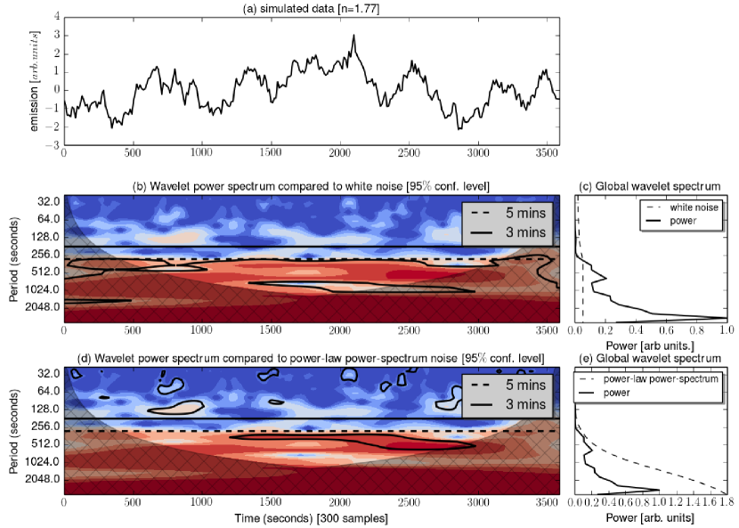
Figure 5.— Comparison of the effect of assuming a white or power-law power spectrum background on the detection of an oscillatory signal for simulated time-series. Plot (a) shows the simulated time-series, generated from a power spectrum $P(f)\propto f^{-1.77}$ and no explicit oscillation included. Plot (b) shows the wavelet power spectrum with the cone-of-influence (shaded area) and regions above the 95% confidence level, assuming the null hypothesis that the time-series is purely noise, and that the noise has the same average power at all wavelet scales. Plot (c) shows the global wavelet power spectrum for this wavelet transform. Plots (d) and (e) are the same as plots (b) and (c) with the null hypothesis that the time-series is purely noise, modeled using an auto-regressive AR(1) model. Such time series assume that the current value in a time-series depends on its previous value plus some Gaussian-distributed noise (Chatfield, 1996.) This time-series model gives rise to a power-law power spectrum of the form $\mbox{power}\propto\nu^{-n}$, where $\nu$ is the frequency of oscillation, and $n$ is its power-law index. The code used in this analysis is an implementation of that described by Torrence & Compo (1998).

Figure 5 illustrates how a time series generated from a random sample from a power-law power spectrum can be mistakenly thought to contain a narrow-band oscillatory signal. The time series in Figure 5(a) is a realization of a random process with a power spectrum of the form $P(f)\approx f^{-1.77}$ with no explicit oscillatory content, using the construction procedure detailed in Vaughan (2010). A different realization of the same process with the same power spectrum would almost certainly generate a different looking time-series, but since there is more power in lower frequencies, lower frequency components are more likely to be visible to the eye compared to higher frequency components. Figure 5(b) shows that if the null hypothesis is that the time-series is purely noise, and that the noise has the same average power at all wavelet scales (for example, if the time-series were pure Gaussian noise), then the 95% confidence level leads to the positive detection of significant oscillatory power in this time series. The detection claim changes if a different null hypothesis is used. Figure 5(d) is the same as Figure 5(b) except with the null hypothesis that the time-series gives rise to a power-law power spectrum of the form $\mbox{power}\propto\nu^{-n}$, where $\nu$ is the frequency of oscillation, and $n$ is its power-law index. This null hypothesis assumption, with the same confidence level, significantly reduces the area in the wavelet transform for which a detection may be claimed. Even with this significantly different background assumption, there is still a significant amount of wavelet power above the 95% confidence level. However, since the data is simulated without an explicit oscillatory component, the high wavelet power must have arisen by chance. The simulated data, along with the results of Section 3, suggest that when examining the wavelet transforms of time-series for wave packets, a background power-law power spectrum should be assumed, along with higher confidence levels (99% or higher), in order to minimize the effects of mistakenly identifying random variations in the background power spectrum as evidence for an oscillatory signal. Since there is a power-law power spectrum in time-series of coronal emission, evidence for the existence of a process that generates narrow-band oscillatory power has to be measured by its power over and above that expected by the power-law power spectrum.

However, even this approach to identifying oscillatory power is not quite complete, as it simply rejects the null hypothesis that the power spectrum can be adequately explained by a power-law power spectrum. Model comparison techniques similar to that described in Section 3 are required to prefer a model with oscillatory content over one without. The difficulty in finding narrow-band features in Fourier power spectra against a background power-law power spectrum has been recognized by Vaughan (2010) in the study of XMM-Newton observations of highly variable Seyfert 1 galaxies. Vaughan (2010) presents a model fitting and comparison technique that is directly applicable to the search for oscillatory power in coronal time-series.

4.2. Implications for coronal seismology and automated oscillation detection algorithms

The discussion of Section 4.1 shows that power-law power spectra have a powerful effect on the claims of a detection of narrow-frequency band oscillations in single time-series. When looking at extended regions of coronal imaging data, evidence for the presence of a propagating wave in the corona is strengthened if it can be shown that narrow frequency-band oscillations occur significantly above the background signal in several neighboring pixels. Spatial extent is the key feature to claim of a detected wave. Coronal seismology derives its observational evidence from such detections, and automated detection algorithms hold out the hope of greatly increasing the number of oscillating regions detected.

Figure 2 shows that time series from individual pixels have power-law like power spectra. This has implications for the design of automated oscillation detection algorithms. Such an algorithm must take into account the nature of the power spectrum. The power-law power spectrum itself lacks an easily definable time-scale at or below which a background trend can be defined. Automated detection algorithms that rely on background trend subtraction, such as Ireland et al. (2010) must therefore look to other reasons to justify a time-scale.

As has been shown above, the assumption of a Gaussian-distributed (white) noise when a power-law power spectrum is actually present, coupled with too low a confidence level, can lead to misleading results when looking for oscillatory signals (Section 4.1 and Figure 5). The detection algorithms outlined in Section 1 have yet to be tested assuming a background power-law power spectrum, and so their efficacy is unknown. De Moortel & McAteer (2004) and Sych & Nakariakov (2008) are wavelet-based approaches, and the discussion Section 4.1 does suggest that a background power-law power spectrum will make a significant difference to the number of wave detections found in the data.

All the automated detection algorithms described above attempt to find individual pixels that are obviously oscillating at some frequency, using the strength of the oscillation at that frequency (compared to some assumption of the background) as the key quantity to measure. These pixels are then clumped together and the quality of the signal is then assessed. The wave coherence detection approach of McIntosh et al. (2008) implement wave detection through finding spatially contiguous regions of the corona which are coherent in a given frequency range. McIntosh et al. (2008) use a symmetric filter to estimate the coherence, in that oscillatory power from either side of the central search frequency contributes the same weight to the final result. The effect of this filter in the presence of a power-law power spectrum may be to bias detections to lower frequencies. Oscillations that are detected propagating along loops are often found by considering distance-time plots (De Moortel et al., 2000; King et al., 2003) and looking for alternating brightening/darkening in those plots as a indicator of a propagating wave. This is essentially a coherence-based approach that involves an implicit assessment of the likelihood that an oscillation has been detected. The basis of the assessment is a judgement that a signal is observed in multiple contiguous pixels. However, the results of Section 3 suggest that each pixel in these plots has a background power-law power spectrum: the discussion of Section 4.1 therefore suggests that the significance of any claimed oscillation is much reduced.

4.3. “Excess” emission

The models fits of Section 3 indicate that Model 2 is preferred over Model 1 as the superior description of the observed Fourier power spectrum. The moss region shows the greatest contribution from the lognormal distribution $G(\nu)$ over the background power-law. De Pontieu et al. (2005) show that it is possible to leak oscillatory power from lower in the atmosphere to the upper reaches of the atmosphere through the simple expedient of tilting the field line. This changes the acoustic cutoff frequency and so allows wave energy to propagate up in to the upper atmosphere. If spectral model $M_{2}$ represents conditions in the solar atmosphere, then it should be possible to infer a distribution of field line angles with the solar surface using De Pontieu et al. (2005) and the observed power distribution $G(\nu)$. This would constrain the distribution of field line angles in the lower atmosphere in different regions of the solar surface.

Another possible cause of the excess emission is the appearance of low-temperature emission lines in the AIA passbands. Such lines are more likely to be due to processes lower down in the solar atmosphere where the amplitude of three and five minute oscillations is larger. This is supported by three dimensional magnetohydrodynamic models of the quiet Sun studied by Martínez-Sykora et al. (2011). It is shown that lower temperature lines can be formed in quiet Sun areas that appear in the AIA 171Å and 193Å wavebands. Martínez-Sykora et al. (2011) find that the AIA 193Å has more significant contributions from non-dominant lines when compared to AIA 171Å. If this were the case, then one would expect that the maximum of the ratio between $G(\nu)/P_{1}(\nu)$ (see Figure 4 and Table 1) would be higher for the AIA 193Å power spectrum than for the AIA 171Å power spectrum, which is not observed. However, Martínez-Sykora et al. (2011) also note that their results are also quite sensitive to the abundances used in their simulations, which may explain the differences between their simulations and the observations presented here.

4.4. Nature of the power-law power spectrum

Power-law power spectrum have been observed in other solar phenomena. As was mentioned above, Auchère et al. (2014) observe power-laws in the integrated emission of small portions of active regions and the quiet Sun as observed in the 195Å passband images from EIT over the frequency range 0.01 - 1 mHz. Also, Gupta (2014) showed power-law power spectra in the intensity at six single points in AIA 171Å coronal plumes extending over the frequency range $0.3\rightarrow 4.0$ mHz. Lower in the solar atmosphere, Reardon et al. (2008) show the presence of power-law Fourier power spectra, in the range 7-20 mHz, in the Doppler velocity of the chromospheric Ca II 854.2 nm line as observed by the Interferometric Bidimensional Spectrometer (IBIS). Further out in the solar atmosphere at 2.1 $R_{sun}$, Bemporad et al. (2008) show the presence of power-law power spectra in Ultraviolet Coronagraph Spectrometer observations of the intensity of Lyman-$\alpha$ in the frequency range $2.6\times 10^{-6}\rightarrow 1.3\times 10^{-4}$ Hz.

The coronal regions studied here also exhibit power-law-like power spectra in the approximate frequency range $0.05\rightarrow 10$ mHz. Under the modeling assumptions of models $M_{1}$ and $M_{2}$, the first contribution to the observed power spectrum is a power-law (which is detectable in all regions up to about 2 mHz). It is present in both wavebands studied and in all the regions, and so parsimony suggests that the mechanism of its creation is both similar and ubiquitous in all similar parts of the solar atmosphere , that is quiet Sun, moss, loop footpoints and above sunspots. Further, Auchère et al. (2014) show that a power-law power spectrum is present in time-series of coronal active region and quiet Sun emission over the frequency range 0.01 - 1 mHz, overlapping with the frequency studied in this paper. We hypothesize that the power-law power spectrum in the coronal 171Å and 193Å emission is due to the sum of a distribution of a large number of events having different amounts of emission. Aschwanden (2011) describes how a power-law power spectrum may obtained from such a distribution, and that argument is outlined below.

Each emission event is modeled as an exponentially decaying function of time $t$

$$f(t)=\frac{E}{T}\exp\left(-\frac{t}{T}\right),$$ (5)

for some timescale $T$ and emission $E$. The corresponding Fourier power spectrum is

$$P(\nu)=\frac{E}{1+(2\pi\nu T)^{2}}.$$ (6)

The total Fourier power spectrum along the line of sight is given by

$$P_{total}(\nu)=\sum_{T}N(T)P_{T}(\nu)$$ (7)

where $N(T)$ is the distribution of time-scales for all the events along the line of sight. Further, if the number of events of a given emission $E$ is assumed to be

$$N(E)\propto E^{-\alpha_{E}}$$ (8)

and the total emission in each event depends on its time scale $T$ such that

$$E\propto T^{1+\gamma}$$ (9)

then it can be shown that the observed power spectrum can be approximated by

$$P_{total}(\nu)\propto\nu^{-(2-\alpha_{E})(1+\gamma)}.$$ (10)

This derivation shows it is possible to generate power-law power spectra using swarms of statistically similar emission events. Equation 10 extends a suggestion by Hudson (1991) that Equation 6 be used to estimate the timescale of a number of smaller heating events with identical timescale $T$ in a sufficiently long span of solar X-ray observations. Hudson (1991) is extended by considering a distribution of heating event timescales (Equation 8) as opposed to a single timescale.

The derivation of the power-law power spectrum Equation 10 shares many similar features with the nanoflare model of energy deposition in the solar atmosphere. In the nanoflare model advanced by Parker (1988), large numbers of small magnetic reconnection events convert the energy in the magnetic field into energy that heats the corona. Nanoflares are hypothesized to be small ($10^{24}-10^{27}$ ergs) yet ubiquitous in the corona. Winebarger et al. (2013) and Testa et al. (2013) analyzing narrowband 193Å images taken by the Hi-C instrument on board a sounding rocket demonstrate the heating of small scale coronal structures that appear to be consistent with scenarios of nanoflare heating due to reconnecting magnetic loops. However, the nanoflare occurence rate, or their energy distribution for the entire solar atmosphere is as yet unknown.

Any modeling or theoretical effort to infer the occurence rate and energy distribution of energy deposition events from the observed emission power-law power spectrum depends strongly on three factors that influence the observation. Firstly, many different loops lie along the line-of-sight in the corona. Each of these may have different emission measures, temperatures and densities. The location of energy deposition may not be the same for each loop (Walsh & Ireland, 2003; Klimchuk, 2006). This implies that attempts to work back from the observed emission to the underlying energy deposition must properly account for these line-of-sight effects.

Secondly, the amount of energy and the wavelengths at which it is radiated is a highly nonlinear function of the energy deposited in each event, depending on the existing plasma properties and the location of the energy deposition in the loop structure. This must all be consistently modeled on each loop and summed over multiple loops to mimic the line-of-sight effects, as noted above. For example, Martínez-Sykora et al. (2011) use a full three-dimensional MHD model to simulate an evolving solar atmosphere and its emission (Gudiksen et al., 2011). Klimchuk et al. (2008); Cargill et al. (2012) have developed a zero-dimensional model of individual strands in a coronal loop that describes the strand’s average temperature, pressure, and density. Such models can be run quickly and so can be used to model hundreds of coronal loops.

Finally, the AIA instrument filter response at the time of the observation must also be understood and modeled in order to understand which emission lines contribute to the final observed image, and ultimately the Fourier power spectrum for each region. O’Dwyer et al. (2010) assume differential emission measure curves for different regions on the Sun (active region, quiet Sun, coronal hole, flaring flasma) and calculate synthetic spectra. These synthetic spectra were convolved with the effective area of each channel, in order to determine the dominant contribution in different regions of the solar atmosphere. However, as noted by Martínez-Sykora et al. (2011), the differential emission measure curves selected by O’Dwyer et al. (2010) are not guaranteed to accurately describe the conditions actually present, and so the fractional contributions of each line in the AIA waveband are estimates only.

These three factors will all have an effect on the inferred properties of the energy deposition rate. The observed power-law power spectrum here, coupled with the emission event hypothesis and a modeling effort that takes account of the factors above, offers a new way to constrain the energy deposition rate in the solar corona. Under the hypothesis, the energy deposition rate can be explored through the distribution of the number of events along the line-of-sight and their temporal dependence, expressed through the parameters $\alpha_{E}$ and $\gamma$ in Equation 8.

5. Conclusions

Time series of AIA 171Å and 193Å images show approximately power law like properties in four representative regions of the corona. It has been shown that the detection of narrow band oscillatory power in the practice of coronal seismology must take in to account the presence of the power-law like power spectrum. Detection thresholds should also increase in order to reduce the number of false positive detections in the presence of power-law like power spectrum. The power spectra have been modelled using three components: a power-law power spectrum, a lognormal component, and a constant background. It is hypothesized that the power-law component is due to the sum along the line of sight of a large number of statistically similar energy deposition events. It is also hypothesized that the lognormal component is due a combination of the channeling of oscillatory power from lower to higher levels of the solar atmosphere and lower temperature emission lines in the AIA 171Å and 193Å bandpasses.

Future studies will include examining power spectra at many more locations on and off the disk. Automated definitions of coronal structures will be used to segment particular coronal features from the data, and so provide improved information of the differences the coronal structure makes to the observed power-law power spectrum. Other AIA wavebands, such as AIA 355Å, 94Å, 131Åand 211Å will be used to look for further evidence of power-law power spectra in different broad temperature ranges in the solar corona. The power-law index in individual pixels will also be determined, and correlated with other physical quantities such as the emission from those pixels. Finally, a better understanding of the source of the power-law power spectrum will come from comparing the Fourier power spectrum of simulated observations to the Fourier power spectrum of the data in all the AIA wave-bands that are sensitive to higher temperatures. This will bring new constraints on the simulations and improve our understanding of the temporal behavior of the solar corona.

Appendix A Fitting models to the mean Fourier power spectra

In order to perform the fit, the noise in the mean Fourier power spectrum (black lines, Figure 4) must be estimated. To do that, the distribution of Fourier power in a region at each frequency must be considered (see Figure 2 for some example distributions). These distributions are constructed by calculating the Fourier power at each pixel in the region, and binning those powers by frequency. However, the Fourier power at a given pixel is not independent of the Fourier power at another pixel. This is because neighbouring pixels are highly likely to be physically connected to each other, and so time-series in neighboring pixels are likely to be strongly correlated (assuming that the background structure exists over at least two pixels). Also, the point spread function of AIA spreads emission in one pixel over on to its neighbors; therefore even neighboring pixels that are not physically connected are still correlated.

Let the standard error in the mean of samples from a distribution be given by $\sigma_{mean}$. It is defined as the standard deviation of the sampling distribution of the mean:

$$\sigma_{mean}=\sigma_{original}/\sqrt{N}$$ (A1)

where $\sigma_{original}$ is the standard deviation of the distribution and $N$ is the sample size. This formula assumes that the measurements taken are all independent of each other, which is not the case for the Fourier power spectra studied here. Hence the value of $N$ cannot be set to the number of pixels in a region.

Hence, the number of effectively independent pixels time-series must be calculated. The dependence of pixels on each other is calculated using the following modeling assumptions. First, a pair of randomly chosen next-nearest neighbor pixels are selected from the region. Next nearest neighbor pixels are chosen as close physical proximity is most likely to express the strongest interdependence. Next, the cross correlation $c(\tau)$ function between two randomly chosen next-nearest neighbor pixels is calculated. The cross correlation coefficient measures the linear dependence of two time series $X(t)$ and $Y(t\pm\tau)$ at different lag times $\tau$. The assumption here is that the linear dependence as measured by the cross-correlation coefficient estimates the actual dependence between time-series. The cross correlation coefficient is used to define a coefficient of independence between the neighbors,

$$\rho=1-\max|c(\tau)|.$$ (A2)

When $\rho$ is 1, the cross-correlation coefficient is zero, and there is no measurable linear dependence between neighboring time series. When $\rho$ is zero, the cross correlation coefficient is $\pm 1$, and the two time-series are linearly dependent on each other. This procedure is repeated 10,000 times. The effective number of pixels $N_{eff}$ is defined as values is defined as

$$N_{eff}=1+\hat{\rho}(N_{pixel}-1).$$ (A3)

where $\hat{\rho}$ is the arithmetic mean of the values of $\rho$ found.

A.1. Model fitting and selection

Equations 1 and 2 are fit to the geometric mean power spectra shown in Figures 4. A Bayesian/Markov chain Monte Carlo package (PyMC version 2.3, Patil, Huard, & Fonnesbeck, 2010) is used to construct the Bayesian posterior and determine model parameter estimates and their uncertainty. If $P_{i,j}$ is the power at Fourier frequency $\nu_{j}$ from Model $i$ then the likelihood $L$ is

$$L=\prod_{j=1}^{N_{f}}\frac{1}{\sqrt{2\pi\sigma_{j}^{2}}}\exp\left(-\frac{(P_{i,j}-D_{j})^{2}}{2\sigma_{j}^{2}}\right)$$ (A4)

where $D_{j}$ is the observed mean Fourier power spectrum at frequency $\nu_{j}$, $N_{f}$ is the number of Fourier frequencies, and $\sigma_{j}$ is the normal distribution width at frequency $\nu_{j}$. Each of the priors for the parameters in each model has a uniform distribution, and are given in Table 2. For some parameters, the logarithm of the model parameter has a uniform distribution, which aids in the exploration of parameter space. Each MCMC chain that was run took 100,000 samples, with burn-in assumed to be at 50,000 samples. The chain is thinned by taking every fifth element in the chain, forming the final sample from which the parameter estimates and their uncertainties are calculated.

Table 2Priors for each of the parameters used in Model 1 (Equation 1) and Model 2 (Equation 2)

parameter	Model 1 and 2	Model 2 only
$\log_{10}A$	$-4.34\rightarrow 2.00$	not applicable
$n$	$1\rightarrow 6$	not applicable
$\log_{10}C$	$-8.68\rightarrow 2.00$	not applicable
$\log_{10}\alpha$	not applicable	$8.68\rightarrow-1.00$
$\beta$	not applicable	$0.1-10$ (mHz)
$\log_{10}\delta$	not applicable	$0.00\rightarrow 3.00$

The mean Fourier power spectra are assumed to be normally distributed with a width given by $\sigma_{mean}$ as calculated above. A five step fitting process is used to fit Models 1 and 2 to the data, and is described below.

1. The posterior is formed by multiplying the likelihood (equation A4) by the priors for $A$, $n$ and $C$ (Table 2). The MCMC sampler is run to fit Model 1, assuming $\sigma_{j}=\sigma_{original,j}$ the width of the distribution of Fourier power at frequency $G(\nu_{j})$. Since the widths $\sigma_{original,j}$ are large it allows the fitting algorithm to converge to an approximate fit solution.

2. The posterior is formed by multiplying the likelihood (equation A4) by the priors for $A$, $n$, and $C$ (Table 2). The MCMC sampler is run to fit Model 1 with $\sigma_{j}=\sigma_{original,j}/sqrt{N_{eff}}$, seeded with estimated parameter values from step 1. This generates a better estimate to the parameters of the model fit. The resulting parameter estimates are given by the mean values of marginal probability distribution functions, and are the final estimates for Model 1. The reduced chi-squared measurement $\chi^{2}_{r}$ for model $M_{1}$ is calculated using the values of $\sigma_{j}$ above.

3. The residuals of the model 1 fit to the data are then used to estimate the model parameters of $G(\nu)$. This is done by (least-squares) fitting $G(\nu)$ to the positive residuals in the frequency range 0.1 - 10 mHz.

4. The MCMC sampler is run to fit Model 2 assuming $\sigma_{j}=\sigma_{original,j}$, seeded with the mean parameter values of Model 1 from step 2 and the estimated $G(\nu)$ model parameters from step 3.

5. The posterior is formed by multiplying the likelihood (equation A4) by all the priors for Model 2 (Table 2). The MCMC sampler is run to fit Model 2 with $\sigma_{j}=\sigma_{original,j}/\sqrt{N_{eff}}$, seeded with estimated parameter values from step 4. The resulting parameter estimates are given by the mean values of marginal probability distribution functions, and are the final estimates for Model 2. The reduced chi-squared measurement $\chi^{2}_{r}$ for model $M_{2}$ is calculated using the values of $\sigma_{j}$ above.

The preferred model is selected using the Akaike Information Criteria (Liddle, 2007), as described in the main text. Conveniently, the AIC is calculated by the PyMC package used to perform the MCMC sampling. The 68% credible intervals for the parameters of the model preferred using the AIC are quoted in Table 1. The upper and lower limits to the credible intervals are found by determining the values beyond which 16% of the probability lies in each wing of the marginal distributions.

References

- Akaike (1974) Akaike, H. 1974, Automatic Control, IEEE Transactions on, 19, 716
- Anić & McAteer (2013) Anić, A., & McAteer, R. T. J. 2013, ApJ, 772, 54
- Aschwanden (2011) Aschwanden, M. J. 2011, Self-Organized Criticality in Astrophysics (Springer-Praxis, Berlin)
- Aschwanden et al. (1999) Aschwanden, M. J., Fletcher, L., Schrijver, C. J., & Alexander, D. 1999, ApJ, 520, 880
- Auchère et al. (2014) Auchère, F., Bocchialini, K., Solomon, J., & Tison, E. 2014, A&A, 563, A8
- Bemporad et al. (2008) Bemporad, A., Matthaeus, W. H., & Poletto, G. 2008, ApJ, 677, L137
- Berghmans & Clette (1999) Berghmans, D., & Clette, F. 1999, Sol. Phys., 186, 207
- Calabro et al. (2013) Calabro, B., McAteer, R. T. J., & Bloomfield, D. S. 2013, Sol. Phys., 286, 405
- Cargill et al. (2012) Cargill, P. J., Bradshaw, S. J., & Klimchuk, J. A. 2012, The Astrophysical Journal, 752, 161
- Chatfield (1996) Chatfield, C. 1996, The Analysis of Time Series An Introduction (Chapman and Hall)
- De Moortel et al. (2002) De Moortel, I., Ireland, J., Hood, A. W., & Walsh, R. W. 2002, A&A, 387, L13
- De Moortel et al. (2000) De Moortel, I., Ireland, J., & Walsh, R. W. 2000, A&A, 355, L23
- De Moortel & McAteer (2004) De Moortel, I., & McAteer, R. T. J. 2004, Sol. Phys., 223, 1
- De Moortel & Nakariakov (2012) De Moortel, I., & Nakariakov, V. M. 2012, Royal Society of London Philosophical Transactions Series A, 370, 3193
- De Pontieu et al. (2005) De Pontieu, B., Erdélyi, R., & De Moortel, I. 2005, ApJ, 624, L61
- De Pontieu et al. (2003) De Pontieu, B., Erdélyi, R., & de Wijn, A. G. 2003, ApJ, 595, L63
- DeForest & Gurman (1998) DeForest, C. E., & Gurman, J. B. 1998, ApJ, 501, L217
- Delaboudinière et al. (1995) Delaboudinière, J.-P., Artzner, G. E., Brunaud, J., et al. 1995, Sol. Phys., 162, 291
- Domingo et al. (1995) Domingo, V., Fleck, B., & Poland, A. I. 1995, Sol. Phys., 162, 1
- Freeland & Handy (1998) Freeland, S. L., & Handy, B. N. 1998, Sol. Phys., 182, 497
- Grechnev (2003) Grechnev, V. V. 2003, Sol. Phys., 213, 103
- Gudiksen et al. (2011) Gudiksen, B. V., Carlsson, M., Hansteen, V. H., et al. 2011, A&A, 531, A154
- Gupta (2014) Gupta, G. R. 2014, A&A, 568, A96
- Handy et al. (1999) Handy, B. N., Acton, L. W., Kankelborg, C. C., et al. 1999, Sol. Phys., 187, 229
- Hudson (1991) Hudson, H. S. 1991, Sol. Phys., 133, 357
- Hunter (2007) Hunter, J. D. 2007, Computing In Science & Engineering, 9, 90
- Ireland et al. (2010) Ireland, J., Marsh, M. S., Kucera, T. A., & Young, C. A. 2010, Sol. Phys., 264, 403
- Ireland et al. (2013) Ireland, J., Tolbert, A. K., Schwartz, R. A., Holman, G. D., & Dennis, B. R. 2013, ApJ, 769, 89
- Jess et al. (2007) Jess, D. B., Andić, A., Mathioudakis, M., Bloomfield, D. S., & Keenan, F. P. 2007, A&A, 473, 943
- King et al. (2003) King, D. B., Nakariakov, V. M., Deluca, E. E., Golub, L., & McClements, K. G. 2003, A&A, 404, L1
- Klimchuk (2006) Klimchuk, J. A. 2006, Sol. Phys., 234, 41
- Klimchuk et al. (2008) Klimchuk, J. A., Patsourakos, S., & Cargill, P. J. 2008, ApJ, 682, 1351
- Lemen et al. (2012) Lemen, J. R., Title, A. M., Akin, D. J., et al. 2012, Sol. Phys., 275, 17
- Lewis (1995) Lewis, J. P. 1995, in Vision interface, Vol. 10, 120–123
- Liddle (2007) Liddle, A. R. 2007, MNRAS, 377, L74
- Martínez-Sykora et al. (2011) Martínez-Sykora, J., De Pontieu, B., Testa, P., & Hansteen, V. 2011, ApJ, 743, 23
- McAteer et al. (2005) McAteer, R. T. J., Gallagher, P. T., Brown, D. S., et al. 2005, ApJ, 620, 1101
- McIntosh et al. (2008) McIntosh, S. W., de Pontieu, B., & Tomczyk, S. 2008, Sol. Phys., 252, 321
- Mumford et al. (2013) Mumford, S., Pérez-Suárez, D., Christe, S., Mayer, F., & Hewett, R. J. 2013, in Proceedings of the 12th Python in Science Conference, ed. S. van der Walt, J. Millman, & K. Huff, 74 – 77
- Nakariakov & King (2007) Nakariakov, V. M., & King, D. B. 2007, Sol. Phys., 241, 397
- Nakariakov et al. (1999) Nakariakov, V. M., Ofman, L., Deluca, E. E., Roberts, B., & Davila, J. M. 1999, Science, 285, 862
- Nakariakov & Verwichte (2005) Nakariakov, V. M., & Verwichte, E. 2005, Living Reviews in Solar Physics, 2, doi:10.12942/lrsp-2005-3
- O’Dwyer et al. (2010) O’Dwyer, B., Del Zanna, G., Mason, H. E., Weber, M. A., & Tripathi, D. 2010, A&A, 521, A21
- Parker (1988) Parker, E. N. 1988, ApJ, 330, 474
- Patil et al. (2010) Patil, A., Huard, D., & Fonnesbeck, C. J. 2010, Journal of Statistical Software, 35, 1
- Pesnell et al. (2012) Pesnell, W. D., Thompson, B. J., & Chamberlin, P. C. 2012, Sol. Phys., 275, 3
- Phillips et al. (2000) Phillips, K. J. H., Read, P. D., Gallagher, P. T., et al. 2000, Sol. Phys., 193, 259
- Pontieu & McIntosh (2010) Pontieu, B. D., & McIntosh, S. W. 2010, The Astrophysical Journal, 722, 1013
- Pérez & Granger (2007) Pérez, F., & Granger, B. E. 2007, Computing in Science & Engineering, 9, 21
- Reardon et al. (2008) Reardon, K. P., Lepreti, F., Carbone, V., & Vecchio, A. 2008, ApJ, 683, L207
- Sych & Nakariakov (2008) Sych, R. A., & Nakariakov, V. M. 2008, Sol. Phys., 248, 395
- Takeuchi (2000) Takeuchi, T. T. 2000, Ap&SS, 271, 213
- Testa et al. (2013) Testa, P., De Pontieu, B., Martínez-Sykora, J., et al. 2013, ApJ, 770, L1
- Tian et al. (2011) Tian, H., McIntosh, S. W., & Pontieu, B. D. 2011, The Astrophysical Journal Letters, 727, L37
- Torrence & Compo (1998) Torrence, C., & Compo, G. P. 1998, Bulletin of the American Meteorological Society, 79, 61
- Uchida (1970) Uchida, Y. 1970, PASJ, 22, 341
- van der Walt et al. (2014) van der Walt, S., Schönberger, J. L., Nunez-Iglesias, J., et al. 2014, PeerJ, 2, e453
- Vaughan (2010) Vaughan, S. 2010, MNRAS, 402, 307
- Walsh & Ireland (2003) Walsh, R. W., & Ireland, J. 2003, A&A Rev., 12, 1
- Winebarger et al. (2013) Winebarger, A. R., Walsh, R. W., Moore, R., et al. 2013, ApJ, 771, 21