A Nearly Optimal Multigrid Method for General Unstructured Grids

Abstract

In this paper, we develop a multigrid method on unstructured shape-regular grids. For a general shape-regular unstructured grid of ${\cal O}(N)$ elements, we present a construction of an auxiliary coarse grid hierarchy on which a geometric multigrid method can be applied together with a smoothing on the original grid by using the auxiliary space preconditioning technique. Such a construction is realized by a cluster tree which can be obtained in ${\cal O}(N\log N)$ operations for a grid of $N$ elements. This tree structure in turn is used for the definition of the grid hierarchy from coarse to fine. For the constructed grid hierarchy we prove that the convergence rate of the multigrid preconditioned CG for an elliptic PDE is $1-{\cal O}({1}/{\log N})$. Numerical experiments confirm the theoretical bounds and show that the total complexity is in ${\cal O}(N\log N)$.

Key words: clustering, multigrid, auxiliary space, finite elements

1 Introduction

We consider a sparse linear system

$$Au=f$$ (1)

that arises from the discretization of an elliptic partial differential equation. In recent decades, multigrid (MG) methods have been well established as one of the most efficient iterative solvers for (1). Moreover, intensive research has been done to analyze the convergence of MG. In particular, it can be proven that the geometric multigrid (GMG) method has linear complexity ${\cal O}(N)$ in terms of computational and memory complexity for a large class of elliptic boundary value problems.

Roughly speaking, there are two different types of theories that have been developed for the convergence of GMG. For the first kind theory that makes critical use of elliptic regularity of the underlying partial differential equations as well as approximation and inverse properties of the discrete hierarchy of grids, we refer to Bank and Dupont [1], Braess and Hackbusch [4], Hackbusch[26], and Bramble and Pasciak[5]. The second kind of theory makes minor or no elliptic regularity assumption, we refer to Yserentant [51], Bramble, Pasciak and Xu [7], Bramble, Pasciak, Wang and Xu [6], Xu [45, 46] and Yserentant [52], and Chen, Nochetto and Xu [15, 49].

The GMG method, however, relies on a given hierarchy of geometric grids. Such a hierarchy of grids is sometimes naturally available, for example, due to an adaptive grid refinement or can be obtained in some special cases by a coarsening algorithm [16]. But in most cases in practice, only a single (fine) unstructured grid is given. This makes it difficult to generate a sequence of nested meshes. To circumvent this difficulty, non-nested geometric multigrid and relevant convergence theories have been developed. One example of such kind of theory is by Bramble, Pasciak and Xu [8]. In this work, optimal convergence theories are established under the assumption that a non-nested sequence of quasi-uniform meshes can be obtained. Another example is the work by Bank and Xu [2] that gives a nearly optimal convergence estimate for a hierarchical basis type method for a general shape-regular grid in two dimensions. This theory is based on non-nested geometric grids that have nested sets of nodal points from different levels.

One feature in the aforementioned MG algorithms and their theories is that the underlying multilevel finite element subspaces are not nested, which is not always desirable from both theoretical and practical points of view. To avoid the non-nestedness, many different MG techniques and theories have been explored in the literature. One such a theory was developed by Xu [47] for a semi-nested MG method with an unstructured but quasi-uniform grid based on an auxiliary grid approach. Instead of generating a sequence of non-nested grids from the initial grid, this method is based on a single auxiliary structured grid whose size is comparable to the original quasi-uniform grid. While the auxiliary grid is not nested with the original grid, it contains a natural nested hierarchy of coarse grids. Under the assumption that the original grid is quasi-uniform, an optimal convergence theory was developed in [47] for second order elliptic boundary problems with Dirichlet boundary conditions.

Totally nested multigrid methods can also be obtained for general unstructured grids, for example, algebraic multigrid (AMG) methods. Most AMG methods, although their derivations are purely algebraic in nature, can be interpreted as nested MG when they are applied to finite element systems based on a geometric grid. AMG methods are usually very robust and converge quickly for Poisson-like problems [9, 34]. There are many different types of AMG methods: the classical AMG [36, 10], smoothed aggregation AMG [40, 43, 12], AMGe [30, 31], unsmoothed aggregation AMG [14, 3] and many others. Highly efficient sequential and parallel implementations are also available for both CPU and GPU systems [27, 11, 44]. AMG methods have been demonstrated to be one of the most efficient solvers for many practical problems [39]. Despite of the great success in practical applications, AMG still lacks solid theoretical justifications for these algorithms except for two-level theories [41, 43, 37, 38, 19, 18, 13]. For a truly multilevel theory, using the theoretical framework developed in [6, 46], Vaněk, Mandel, and Brezina [42] provide a theoretical bound for the smoothed aggregation AMG under some assumption about the aggregations. Such an assumption has been recently investigated in [13] for aggregations that are controlled by auxiliary grids that are similar to those used in [47].

The aim of this paper is to extend the algorithm and theory in Xu [47] to shape regular grids that are not necessarily quasi-uniform. The lack of quasi-uniformity of the original grid makes the extension nontrivial for both the algorithm and the theory. First, it is difficult to construct auxiliary hierarchical grids without increasing the grid complexity, especially for grids on complicated domains. The way we construct the hierarchical structure is to generate a cluster tree, based on the geometric information of the original grid [22, 24, 23, 21]. This auxiliary cluster tree has also been used as a coarsening process of the UA-AMG [44]. Secondly, it is also not straightforward to establish optimal convergence for the geometric multigrid applied to hierarchy of auxiliary grids that can be highly locally refined.

The rest of the paper is organized as follows. In §2, we discuss some basic assumptions on the given triangulation and review multigrid theories and the auxiliary space method. An abstract analysis is provided based on four assumptions. In §3 we introduce the detailed construction of the structured auxiliary space by an auxiliary cluster tree and an improved treatment of the boundary region for Neumann boundary conditions. In §4, we describe the auxiliary space multgrid preconditioner (ASMG) and estimate the condition number by verifying the assumptions of the abstract theory. Finally, in §5, we provide some numerical examples to verify our theory.

For simplicity of exposition, the algorithm and theory are presented in this paper for the two dimensional case by using a quadtree. They can be generalized for the three dimensional case without intrinsic difficulties by using an octree.

2 Preliminaries

We present a multigrid method for second order elliptic problems on a complicated domain $\Omega\subset\mathbb{R}^{d}$ ($1\leq d\leq 3$). Let $\mathcal{V}$ be the initial Hilbert space with inner product $a(\cdot,\cdot)$ and energy norm $\parallel\cdot\parallel_{A}$. The variational problem we want to solve is

$$Find\ v\in\mathcal{V}\ s.t.\ \ a(u,v):=\langle Au,v\rangle=\langle f,v\rangle\qquad\forall v\in\mathcal{V}$$ (2)

In order to simplify the presentation, we restrict ourselves to the Poisson problem discretized by piecewise linear finite elements. Assume that the nodal basis functions of $\mathcal{V}$ are $\{\varphi_{i}\}_{i\in{\cal J}}$ and the local elements supporting patch of $\varphi_{i}$ is $\omega_{i}$ where ${\cal J}$ is the node index set. For any $v\in\mathcal{V}$, there exists $\xi\in\mathbb{R}^{N}$ such that $v=\sum_{i\in{\cal J}}\xi_{i}\varphi_{i}$. In this case, the system matrix $A$ has entries of the form

$$a_{i,j}=\int_{\Omega}(\nabla\varphi_{i}(x),\nabla\varphi_{j}(x))dx$$

with basis functions $\varphi_{i}(x)$ that are continuous and piecewise affine on triangles $\tau_{\nu},\nu\in{\cal I}:=\{1,\ldots,N\}$ of the triangulation $\mathcal{T}$ of the polygonal and connected domain $\Omega\subset\mathbb{R}^{d}$,

$$\overline{\Omega}=\bigcup_{\nu\in{\cal I}}\overline{\tau_{\nu}}$$

2.1 Properties of the triangulation

The triangulation is assumed to be conforming and shape-regular in the sense that the ratio of the circumcircle and inscribed circle is bounded uniformly [17], and it is a K-mesh in the sense that the ratio of diameters between neighboring elements is bounded uniformly. All elements $\tau_{i}$ are assumed to be shape-regular but not necessarily quasi-uniform, so the diameters can vary globally and allow a strong local refinement.

The vertices of the triangulation are denoted by $(p_{j})_{j\in{\cal J}}$. Some of the vertices are Dirichlet nodes, ${\cal J}_{D}\subset{\cal J}$, where we impose essential Dirichlet boundary conditions, and some are Neumann vertices, ${\cal J}_{N}\subset{\cal J}$, where we impose natural Neumann boundary conditions.

The following construction will be given for the case $d=2$, but a generalisation to $d>2$ is straightforward .

For each of the triangles $\tau_{i}\in\mathcal{T}$, we use the barycenter

$$\xi_{i}:=\frac{p_{1}(\tau_{i})+p_{2}(\tau_{i})+p_{3}(\tau_{i})}{3},$$

where $p_{1}(\tau_{i}),p_{2}(\tau_{i}),p_{3}(\tau_{i})\in\mathbb{R}^{2}$ are the three vertices of the triangle $\tau_{i}$, as in Figure 1.

Notation: We denote the minimal distance between the triangle barycenters of the grid by

$$h:=\min_{i,j\in{\cal I}}\|\xi_{i}-\xi_{j}\|_{2}.$$

The diameter of $\Omega$ is denoted by

$$H:=\max_{x,y\in\Omega}\|x-y\|_{2}.$$

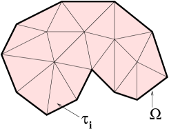
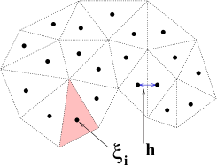
Figure 1: Left: The triangulation $\mathcal{T}$ of $\Omega$ with elements $\tau_{i}$. Right: The barycenters $\xi_{i}$ (dots) and the minimal distance $h$ between barycenters.

In order to prove the desired nearly linear complexity estimate, we have to assume that the refinement level of the grid is algebraically bounded in the following sense.

Assumption 1.

We assume that $H/h\mathrel{\hbox{$\hbox{\raise 0.9pt\hbox{$=$}}\kern-7.7778pt\raise-3.5pt\hbox{$\sim$}$}}N^{q}$ for a small number $q$, e.g. $q=2$.

The above assumption allows an algebraic grading towards a point but it forbids a geometric grading. The assumption is sufficient but not necessary: the construction of the auxiliary grids might still be of complexity ${\cal O}(N\log N)$ or less if Assumption 1 is not valid, but it would require more technical assumptions in order to prove this.

2.2 Auxiliary space preconditioning theory

The auxiliary space method, developed in [33, 47], is for designing preconditioners by using the auxiliary spaces which are not necessarily subspaces of the original space. Here, the original space is the finite element space $\mathcal{V}$ for the given grid $\mathcal{T}$ and the preconditioner is the multigrid method on the sequence $(V_{\ell})_{\ell=1}^{J}$ of FE spaces for the auxiliary grids $({\mathcal{T}}_{\ell})_{\ell=1}^{J}$.

The idea of the method is to generate an auxiliary space $V$ with inner product $\tilde{a}(\cdot,\cdot)=\langle\tilde{A}\cdot,\cdot\rangle$ and energy norm $\parallel\cdot\parallel_{\tilde{A}}$. Between the spaces there is a suitable linear transfer operator $\Pi:V\mapsto\mathcal{V}$, which is continuous and surjective. $\Pi^{t}:\mathcal{V}\mapsto V$ is the dual operator of $\Pi$ in the default inner products

$$\langle\Pi^{t}u,\tilde{v}\rangle=\langle u,\Pi\tilde{v}\rangle,\quad\text{for all }u\in\mathcal{V},\tilde{v}\in V.$$

In order to solve the linear system $Ax=b$, we require a preconditioner B defined by

$$B:=S+\Pi\tilde{B}\Pi^{t},$$ (3)

where $S$ is the smoother and $\tilde{B}$ is the preconditioner of $\tilde{A}$.

The estimate of the condition number $\kappa(BA)$ is given below.

Theorem 1.

Assume that there are nonnegative constants $c_{0},c_{1}$, and $c_{s}$, such that

1. the smoother $S$ is bounded in the sense that

   $$\quad\|v\|_{A}\leq c_{s}\|v\|_{S^{-1}}\qquad\forall v\in\mathcal{V},$$ (4)

2. the transfer operator $\Pi$ is bounded,

   $$\|\Pi w\|_{A}\leq c_{1}\|w\|_{\tilde{A}}\qquad\forall w\in V,$$ (5)

3. the transfer is stable, i.e. for all $v\in\mathcal{V}$ there exists $v_{0}\in\mathcal{V}$ and $w\in V$ such that

   $$\quad v=v_{0}+\Pi w\quad\text{ and }\quad\|v_{0}\|_{S^{-1}}+\|w\|_{\tilde{A}}\leq c_{0}\|v\|_{A},\quad\mbox{and}$$ (6)

4. the preconditioner $\tilde{B}$ on the auxiliary space is optimal, i.e. for any $\tilde{v}\in V$, there exists $m_{1}>m_{0}>0$, such that

   $$m_{0}\|\tilde{v}\|^{2}_{\tilde{A}}\leq(\tilde{B}\tilde{A}\tilde{v},\tilde{v})\leq m_{1}\|\tilde{v}\|^{2}_{\tilde{A}}.$$ (7)

Then, the condition number of the preconditioned system defined by (3) can be bounded by

$$\kappa(BA)\leq\frac{m_{1}}{m_{0}}c_{0}^{2}(c_{s}^{2}+c_{1}^{2}).$$ (8)

We also can combine the smoother S and the auxiliary grid correction multiplicatively with a preconditioner $B$ in the form [29, 28]

$$I-B_{co}A=(I-S^{T}A)(I-BA)(I-SA)$$ (9)

which leads to Algorithm 1. The combined preconditioner, under suitable scaling assumptions performs no worse than its components.

Algorithm 1 Multiplicative Auxiliary Space Iteration Step

  Given S, $B$, and an initial iterate $u^{k,0}:=u^{k}$

  (1) $u^{k,1}:=u^{k,0}-S(b-Au^{k,0})$;

  (2) $u^{k,2}:=u^{k,1}-B(b-Au^{k,1})$;

  (3) $u^{k+1}:=u^{k,2}-S^{T}(b-Au^{k,2})$;

  return  Improved approximate solution $u^{k+1}$.

Theorem 2.

Suppose there exists $\rho\in[0,1)$ such that for all $v\in V$, we have

$$\|(I-SA)v\|_{A}^{2}\leq\rho\|v\|^{2}_{A},$$

then the multiplicative preconditioner $B_{co}$ yields the bound

$$\kappa(B_{co}A)\leq\frac{(1-m_{1})(1-\rho)+m_{1}}{(1-m_{0})(1-\rho)+m_{0}},$$ (10)

for the condition number, and

$$\kappa(B_{co}A)\leq\kappa(BA).$$ (11)

According to Theorem 1 and 2, our goal is to construct an auxiliary space $V$ in which we are able to define an efficient preconditioner. The preconditioner will be the geometric multigrid method on a suitably chosen hierarchy of auxiliary grids. Additionally, the space has to be close enough to $\mathcal{V}$ so that the transfer from $\mathcal{V}$ to $V$ fulfils (5) and (6). This goal is achieved by a density fitting of the finest auxiliary grid $\mathcal{T}_{J}$ to $\mathcal{T}$. In order to prove (7), we use the multigrid theory for the auxiliary grids $\{\mathcal{T}_{\ell}\}_{\ell=1}^{J}$ from the viewpoint of the method of subspace corrections.

2.3 An abstract multigrid theory

In the spirit of divide and conquer, we can decompose any space $V$ as the summation of subspaces $V=\sum_{i=0}^{L}V_{i},\ V_{i}\subset V$. Since $\sum_{i=0}^{L}V_{i}$ may not be a direct sum, the decomposition $u=\sum_{i=0}^{L}u_{i}$ is not necessarily unique for $u\in V$.

We will use the following operators, for $i=1,\ldots,L$:

• $Q_{i}:V\rightarrow V_{i}\quad$ the projection in the $L_{2}$ inner product $(\cdot,\cdot)$;

• $I_{i}:V_{i}\rightarrow V\quad$ the natural inclusion to $V$;

• $P_{i}:V\rightarrow V_{i}\quad$ the projection in the inner product $(\cdot,\cdot)_{A}$;

• $A_{i}:V_{i}\rightarrow V_{i}\quad$ the restriction of A to the subspace $V_{i}$;

• $R_{i}:V_{i}\rightarrow V_{i}\quad$ an approximation of $(A_{i})^{-1}$ which means the smoother;

• $T_{i}:V\rightarrow V_{i}\quad$ $T_{i}=R_{i}Q_{i}A=R_{i}A_{i}P_{i}$.

For any $u\in V$ and $u_{i},v_{i}\in V_{i}$, these operators fulfil the trivial equalities

$$(Q_{i}u,v_{i})=(u,I_{i}v_{i})=(I_{i}^{t}u,v_{i}),$$

$$(A_{i}P_{i}u,v_{i})=a(u,v_{i})=(Q_{i}Au,v_{i}),$$

$$(A_{i}u_{i},v_{i})=a(u_{i},v_{i})=(Au_{i},v_{i})=(Q_{i}AI_{i}u_{i},v_{i}).$$

Assume we know the value of $u^{k}$, if we perform the subspace correction in a successive way, it reads in operator form as

$$v^{0} =u^{k},$$

$$\quad v^{i+1} =v^{i}+I_{i}R_{i}Q_{i}(f-Av^{i}),i=1,\cdots,L,$$

$$\quad u^{k+1} =v^{L+1}$$

The corresponding error equation is

$$(I-BA)u=u-u^{k+1}=\left[\prod_{i=1}^{L}(I-I_{i}R_{i}Q_{i}A)\right](u-u^{k}).$$

Suppose that we have nested finite element spaces: $V_{0}\subset V_{1}\subset V_{2}\subset\cdots\subset V_{J}=V$ and $\{\varphi_{\ell,i}\}$ as the basis functions of $V_{\ell}$. Define $V_{k,i}:=span\{\varphi_{k,i}\}$. Then, $\sum_{\ell,i}V_{\ell,i}$ is the decomposition of $V_{J}$. Then given $v\in V_{J}$, we have the decomposition $v=\sum_{\ell,j}v_{\ell,j}$. Similarly define $P_{\ell,i}$ as the projection from $V_{J}$ to $V_{\ell,i}$. In this case, the successive subspace correction method for this decomposition is nothing but the simple Gauss-Seidel iteration. This algorithm is sometimes called the backslash ($\backslash$) cycle. A V-cycle algorithm is obtained from the backslash cycle by performing more smoothings after the coarse grid corrections. Such an algorithm, roughly speaking, is like a backslash ($\backslash$) cycle plus a slash ($/$) (a reversed backslash) cycle. It is simple to show that the convergence of the V-cycle is a consequence of the convergence of the backslash cycle. The detailed algorithm is given in Algorithm 2.

Algorithm 2 Geometric Multigrid Method

  For $\ell=0$, define $B_{0}=A_{0}^{-1}$. Assume that $B_{\ell-1}:V_{\ell-1}\rightarrow V_{\ell-1}$ is defined. We shall now define $B_{\ell}:V_{\ell}\rightarrow V_{\ell}$ which is an iterator for the equation of the form

$$A_{\ell}u=f.$$

  pre-smoothing: For $u^{0}=0$ and $k=1,2,\cdots,\nu$

$$u^{k}=u^{k-1}+R_{\ell}(f-A_{\ell}u^{k-1})$$

  Coarse grid correction: $e_{\ell-1}\in V_{\ell-1}$ is the approximate solution of the residual equation $A_{\ell-1}e=Q_{\ell-1}(f-A_{\ell}u^{\nu})$ by the iterator $B_{\ell-1}$:

$$u^{\nu+1}=u^{\nu}+e_{\ell-1}=u^{\nu}+B_{\ell-1}Q_{\ell-1}(g-Au^{\nu}).$$

  post-smoothing: For $k=\nu+2,2,\cdots,2\nu$

$$u^{k}=u^{k-1}+R_{\ell}(f-A_{\ell}u^{k-1})$$

Now we present a convergence analysis based on three assumptions.

(T) Contraction of Subspace Error Operator:

There exists $\rho<1$ such that

$$\|I-T_{i}\|_{A_{i}}\leq\rho\qquad\text{for all }i=1,\ldots,L.$$

(A1) Stable Decomposition:

For any $v\in V$, there exists a decomposition

$$v=\sum_{i=1}^{L}v_{i},\quad v_{i}\in V_{i},i=1,\ldots,L,\qquad\text{such that }\,\sum_{i=1}^{L}\|v_{i}\|^{2}_{A_{i}}\leq K_{1}\|v\|^{2}_{A}.$$

(A2) Strengthened Cauchy-Schwarz (SCS) Inequality:

For any $u_{i},v_{i}\in V_{i},i=1,\ldots,L$

$$\left|\sum_{i=1}^{L}\sum_{j=i+1}^{L}(u_{i},v_{j})_{A}\right|\leq K_{2}\left(\sum_{i=1}^{L}\|u_{i}\|^{2}_{A}\right)^{1/2}\left(\sum_{j=1}^{L}\|v_{j}\|^{2}_{A}\right)^{1/2}.$$

The convergence theory of the method is as follows.

Theorem 3.

Let $V=\sum_{i=1}^{L}V_{i}$ be a decomposition satisfying assumptions (A1) and (A2), and let the subspace smoothers $R_{i}$ satisfy (T). Then

$$\left\|\prod_{i=1}^{L}(I-I_{i}R_{i}Q_{i}A)\right\|^{2}_{A}\leq 1-\frac{1-\rho^{2}}{2K_{1}(1+(1+\rho)^{2}K_{2}^{2})}.$$

The proof can be found from [49, 15], which is simplified by using the XZ identity [50].

3 Construction of the auxiliary grid-hierarchy

In this section, we explain how to generate a hierarchy of auxiliary grids based on the given (unstructured) grid $\mathcal{T}$. The idea is to analyse and split the element barycenters by their geometric position regardless of the initial grid structure. Our aim is to obtain a structured hierarchy of grids that preserves some properties of the initial grid, e.g. the local mesh size. A similar idea has already been applied in [20, 32, 44].

3.1 Clustering and auxiliary box-trees

We build an auxiliary tree structure by a geometrically regular subdivision of boxes. For the initial step we choose a (minimal) square bounding box of the domain $\Omega$:

$$\mathcal{B}^{1}:=[a_{1},b_{1})\times[a_{2},b_{2})\supset\Omega,\qquad|b_{1}-a_{1}|=|b_{2}-a_{2}|.$$

Define the level of $\mathcal{B}^{1}$ to be $g(\mathcal{B}^{1})=1$. Then we subdivide $\mathcal{B}^{1}$ regularly, thus obtaining four children $\mathcal{B}^{2}_{1},\mathcal{B}^{2}_{2},\mathcal{B}^{2}_{3},\mathcal{B}^{2}_{4}$:

$$\mathcal{B}^{2}_{2}=[a_{1},b_{1}^{\prime})\times[a_{2}^{\prime},b_{2}), \mathcal{B}^{2}_{3}=[a_{1}^{\prime},b_{1})\times[a_{2}^{\prime},b_{2}),$$

$$\mathcal{B}^{2}_{1}=[a_{1},b_{1}^{\prime})\times[a_{2},b_{2}^{\prime}), \mathcal{B}^{2}_{4}=[a_{1}^{\prime},b_{1})\times[a_{2},b_{2}^{\prime}),$$

where $a_{1}^{\prime}=b_{1}^{\prime}:=(a_{1}+b_{1})/2$ and $a_{2}^{\prime}=b_{2}^{\prime}:=(a_{2}+b_{2})/2$. The level of $\mathcal{B}^{2}_{i}$ is $g(\mathcal{B}^{2}_{i})=g(\mathcal{B}^{1})+1=2$, where $i=1,2,3,4$. Finally, we apply the same subdivision process recursively, starting with $\mathcal{B}^{2}_{1},\ldots,\mathcal{B}^{2}_{4}$ and define the level of the boxes $\mathcal{B}^{\ell}_{i}$ recursively (cf. Figure 2). This yields an infinite tree $T_{\mathrm{box}}$ with root $\mathcal{B}^{1}$. Letting $\mathcal{B}^{\ell}_{j}$ denote a box in this tree, we can define the cluster $t$, which is a subset of ${\cal I}$, by

$$t^{\ell}_{j}:=t(\mathcal{B}^{\ell}_{j}):=\{i\in\mathcal{I}\mid\xi_{i}\in\mathcal{B}^{\ell}_{j}\}.$$

This yields an infinite cluster tree with root $t(\mathcal{B}^{1})$. We construct a finite cluster tree $T_{\cal I}$ by not subdividing nodes which are below a minimal cardinality $n_{\rm min}$, e.g. $n_{\rm min}:=3$. Define the nodes which have no child nodes as the leaf nodes. The cardinality $\#t^{\ell}_{j}=\#t(\mathcal{B}^{\ell}_{j})$ is the number of the barycenters in $\mathcal{B}^{\ell}_{j}$. Leaves of the cluster tree contain at most $n_{\rm min}$ indices. For any leaf node, its parent node contains at least 4 barycenters, then the total number of leaf nodes is bounded by the number of barycenters $N$.

Figure 2: Tree of regular boxes with root $\mathcal{B}^{1}$. The black dots mark the corresponding barycenters $\xi_{i}$ of the triangles $\tau_{i}$. Boxes with less than three points $\xi_{i}$ are leaves.

Remark 1.

The size of a leaf box $\mathcal{B}_{j}$ can be much larger than the size of triangles $\tau_{j}$ that intersect with $\mathcal{B}_{j}$ since a large box $\mathcal{B}_{j}$ may only intersect with one very small element and will not be further subdivided.

Lemma 1.

Suppose Assumption 1 holds, the complexity for the construction of $T_{\cal I}$ is ${\cal O}(qN\log N)$.

Proof.

First, we estimate the depth of the cluster tree. Let $t=t({\cal B}_{\nu})\in T_{\cal I}$ be a node of the cluster tree and $\#t>n_{\rm min}$. By definition the distance between two nodes $\xi_{i},\xi_{j}\in t$ is at least

$$\|\xi_{i}-\xi_{j}\|_{2}\geq h.$$

Therefore, the box ${\cal B}_{\nu}$ has a diameter of at least $h$. After each subdivision step the diameter of the boxes is exactly halved. Let $\ell$ denote the number of subdivisions after which ${\cal B}_{\nu}$ was created. Then

$${\rm diam}({\cal B}_{\nu})=2^{-\ell}{\rm diam}({\cal B}^{1}).$$

Consequently, we obtain

$$h\leq{\rm diam}({\cal B}_{\nu})=2^{-\ell}{\rm diam}({\cal B}^{1})\leq 2^{-\ell}\sqrt{2}H$$

so that by Assumption 1,

$$\ell\lesssim\log(H/h)\mathrel{\hbox{$\hbox{\raise 0.9pt\hbox{$=$}}\kern-7.7778pt\raise-3.5pt\hbox{$\sim$}$}}q\log N.$$

Therefore the depth of $T_{\cal I}$ is in ${\cal O}(q\log N)$.

Next, we estimate the complexity for the construction of $T_{\cal I}$. The subdivision of a single node $t\in T_{\cal I}$ and corresponding box ${\cal B}_{\nu}$ is of complexity $\#t$. On each level of the tree $T_{\cal I}$, the nodes are disjoint, so that the subdivision of all nodes on one level is of complexity at most ${\cal O}(N)$. For all levels this sums up to at most ${\cal O}(qN\log N)$. ∎

Remark 2.

The boxes used in the clustering can be replaced by arbitrary shaped elements, e.g. triangles/tetrahedra or anisotropic elements — depending on the application or operator at hand. For ease of presentation we restrict ourselves to the case of boxes.

Remark 3.

The complexity of the construction can also be bounded from below by ${\cal O}(N\log N)$, as is the case for a uniform (structured) grid. However, this complexity arises only in the construction step and this step will typically be of negligible complexity.

Notice that the tree of boxes is not the regular grid that we need for the multigrid method. A further refinement as well as deletion of elements is necessary.

3.2 Closure of the auxiliary box-tree

The hierarchy of box-meshes from Figure 2 is exactly what we want to construct: each box has at most one hanging node per edge, namely, the fineness of two neighbouring boxes differs by at most one level. In general this is not fulfilled.

We construct the grid hierarchy of nested uniform meshes starting from a coarse mesh $\sigma^{(0)}$ consisting of only a single box $\mathcal{B}^{1}=[a_{1},b_{1})\times[a_{2},b_{2})$, the root of the box tree. All boxes in the meshes $\sigma^{(1)},\ldots,\sigma^{(J)}$ to be constructed will either correspond to a cluster $t$ in the cluster tree or will be created by refinement of a box that corresponds to a leaf of the cluster tree.

Let $\ell\in\{1,\ldots,J\}$ be a level that is already constructed (the trivial start $\ell=1$ of the induction is given above).

We mark all elements of the mesh which are then refined regularly. Let $\mathcal{B}^{\ell}_{\nu}$ be an arbitrary box in $\sigma^{(\ell)}$. The box $\mathcal{B}^{\ell}_{\nu}$ corresponds to a cluster $t_{\nu}=t(\mathcal{B}^{\ell}_{\nu})\in T_{\cal I}$. The following two situations can occur:

• If $\#t_{\nu}>n_{\rm min}$ then $\mathcal{B}^{\ell}_{\nu}$ is marked for refinement.

• If $\#t_{\nu}\leq n_{\rm min}$, e.g. $t_{\nu}=\emptyset$, then $\mathcal{B}^{\ell}_{\nu}$ is not marked in this step.

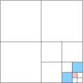
Figure 3: The subdivision of the marked (red) box on level $\ell$ would create two boxes (blue) with more than one hanging node at one edge.

After processing all boxes on level $\ell$, it may occur that there are boxes on level $\ell-1$ that would have more than one hanging node on an edge after refinement of the marked boxes, cf. Figure 3. Since we want to avoid this, we have to perform a closure operation for all such elements and for all coarser levels $\ell-1,\ldots,1$.

• Let ${\cal L}^{(\ell-1)}$ be the set of all boxes on level $\ell-1$ having too many hanging nodes. All of these are marked for refinement. By construction a single refinement of each box is sufficient. However, a refinement on level $\ell-1$ might then produce too many hanging nodes in a box on level $\ell-2$. Therefore, we have to form the lists ${\cal L}^{(j)}$, $j=\ell-1,\ldots,1$ of boxes with too many hanging nodes successively on all levels and mark the elements.

• At last we refine all boxes (on all levels) that are marked for refinement.

The result of the closure operation is depicted in Figure 4.

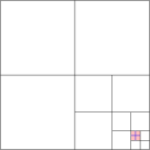
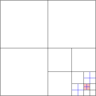
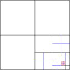
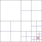
Figure 4: The subdivision of the red box makes it necessary to subdivide nodes on all levels.

Each of the boxes in the closed grids lives on a unique level $\ell\in\{1,\ldots,J\}$. It is important that a box is either refined regularly (split into four successors on the next level) or it is not refined at all. For each box that is marked in step 1, there are at most ${\cal O}(\log N)$ boxes marked during the closure step 3.

Lemma 2.

The complexity for the construction and storage of the (finite) box tree with boxes $\mathcal{B}^{\ell}_{\nu}$ and corresponding cluster tree $T_{\cal I}$ with clusters $t_{\nu}=t(\mathcal{B}^{\ell}_{\nu})$ is of complexity ${\cal O}(N\log N)$, where $N$ is the number of barycenters, i.e., the number of triangles in the triangulation $\tau$.

Proof.

For the level $\ell$ of the tree, let $n_{\ell}$ be the number of leaf boxes and $m_{\ell}$ be the boxes which have child boxes. Accordingly, the total number of the boxes on level $\ell$ is $n_{\ell}+m_{\ell}$. By definition,

$$n_{\ell}+m_{\ell}=4m_{\ell-1},$$

where $\ell\geq 2$ and $n_{1}+m_{1}=m_{1}=1$. Since $\sum_{\ell=1}^{J}n_{\ell}\lesssim N,$ we have

$$N\gtrsim\sum_{\ell=1}^{J}n_{\ell}=\sum_{\ell=2}^{J}(4m_{\ell-1}-m_{\ell})=3\sum_{\ell=1}^{J}m_{\ell}+1.$$

As a result,

$$\sum_{\ell=1}^{J}m_{\ell}\lesssim N.$$

The total work for generating the tree is $\sum_{\ell=1}^{J}n_{\ell}+m_{\ell}\lesssim N$.

Given $\ell$, let $\alpha_{\ell}$ denote the number of boxes in $\mathcal{L}^{(\ell-1)}$ (the set of boxes that have more than 1 hanging node). Since every box in $\mathcal{L}^{(\ell-1)}$ has to be a leaf box, we have $\alpha_{\ell}\leq n_{\ell}$. As the process of closing each hanging node will go through at most two boxes in any given level, the total number of the marked boxes in this closure process is bounded by

$$\sum_{\ell=1}^{J}2J\alpha_{\ell}\lesssim JN\lesssim N\log N.$$

∎

3.3 Construction of a conforming auxiliary grid hierarchy

At last, we create a hierarchy of nested conforming triangulations by subdivision of the boxes and by discarding those boxes that lie outside the domain $\Omega$. For any box $\mathcal{B}_{\nu}$ there can be at most one hanging node per edge. The possible situations and corresponding local closure operations are presented in Figure 5.

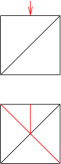
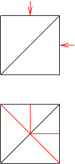
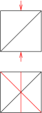
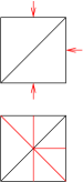
Figure 5: Hanging nodes can be treated by a local subdivision within the box $\mathcal{B}_{\nu}$. The top row shows a box with $1,2,2,3,4$ hanging nodes, respectively, and the bottom row shows the corresponding triangulation of the box.

The closure operation introduces new elements on the next finer level.

The final hierarchy of triangular grids $\sigma^{(1)},\ldots,\sigma^{(J)}$ is nested and conforming without hanging nodes. All triangles have a minimum angle of $45$ degrees, i.e., they are shape-regular, cf. Figure 6.

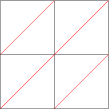
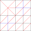
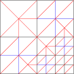
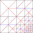
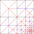
level 1             level 2             level 3             level 4             level 5

Figure 6: The final hierarchy of nested grids. Red edges were introduced in the last (local) closure step.

The triangles in the quasi-regular meshes $\sigma^{(1)},\ldots,\sigma^{(J)}$ have the following properties:

1. All triangles in $\sigma^{(1)},\ldots,\sigma^{(J)}$ that have children which are themselves further subdivided, are refined regularly (four congruent successors) as depicted here.

   

2. Each triangle $\sigma_{i}\in\sigma^{(j)}$ that is subdivided but not regularly refined, has successors $\sigma_{i}^{\prime}$ that will not be further subdivided.

The hierarchy of grids constructed so far covers on each level the whole box $\cal B$. This hierarchy has now to be adapted to the boundary of the given domain $\Omega$. In order to explain the construction we will consider the domain $\Omega$ and triangulation $\mathcal{T}$ ($5837$ triangles) from Figure 7.

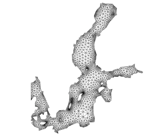
Figure 7: A triangulation of the Baltic sea with local refinement and small inclusions.

The triangulation consists of shape-regular elements, it is locally refined, it contains many small inclusions, and the boundary $\Gamma$ of the domain $\Omega$ is rather complicated.

3.4 Adaptation of the auxiliary grids to the boundary

The Dirichlet boundary: On the Dirichlet boundary we want to satisfy homogeneous boundary conditions (b.c.), i.e., $u|_{\Gamma}=0$ (non-homogeneous b.c. can trivially be transformed to homogeneous ones). On the given fine triangulation $\tau$ this is achieved by use of basis functions that fulfil the b.c. Since the auxiliary triangulations $\sigma^{(1)},\ldots,\sigma^{(J)}$ do not necessarily resolve the boundary, we have to use a slight modification.

Definition 1 (Dirichlet auxiliary grids).

We define the auxiliary triangulations $\mathcal{T}^{D}_{\ell}$ by

$$\mathcal{T}^{D}_{\ell}:=\{\tau\in\sigma^{(\ell)}\mid\tau\subset\Omega\},\quad\ell=1,\ldots,J.$$

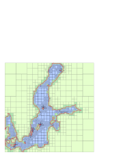
level 3                           level 4                           level 5

Figure 8: The boundary $\Gamma$ of $\Omega$ is drawn as a red line, boxes non-intersecting $\Omega$ are light green, boxes intersecting $\Gamma$ are dark green, and all other boxes (inside of $\Omega$) are blue.

In Figure 8 the Dirichlet auxiliary grids are formed by the blue boxes. All other elements (light green and dark green) are not used for the Dirichlet problem. On an auxiliary grid we impose homogeneous Dirichlet b.c. on the boundary

$$\Gamma_{\ell}:=\partial\Omega^{D}_{\ell},\qquad\Omega^{D}_{\ell}:=\cup_{\tau\in\mathcal{T}^{D}_{\ell}}\bar{\tau}.$$

The auxiliary grids are still nested, but the area covered by the triangles grows with increasing the level number:

$$\Omega^{D}_{1}\subset\cdots\subset\Omega^{D}_{J}\subset\Omega,\qquad\Omega^{D}_{\ell}:=\bigcup\{\tau\in\mathcal{T}^{D}_{\ell}\}$$

The Neumann boundary: On the Neumann boundary we want to satisfy natural (Neumann) b.c., i.e., $\partial_{n}u|_{\Gamma}=0$. For the auxiliary triangulations $\sigma^{(1)},\ldots,\sigma^{(J)}$, we will approximate the true b.c. by the natural b.c. on an auxiliary boundary.

Definition 2 (Neumann auxiliary grids).

Define the auxiliary triangulations $\mathcal{T}^{N}_{1},\ldots,\mathcal{T}^{N}_{J}$ by

$$\mathcal{T}^{N}_{\ell}:=\{\tau\in\sigma^{(\ell)}\mid\tau\cap\Omega\neq\emptyset\},\quad\ell=1,\ldots,J.$$

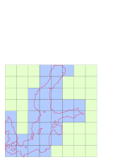
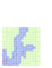
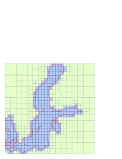
level 3                           level 4                           level 5

Figure 9: The boundary $\Gamma$ of $\Omega$ is drawn as a red line, boxes non-intersecting $\Omega$ are light green, and all other boxes (intersecting $\Omega$) are blue.

In Figure 9 the Neumann auxiliary grids are formed by the blue boxes. All other elements (light green) are not used for the Neumann problem. On an auxiliary grid we impose natural Neumann b.c., the auxiliary grids are non-nested. The area covered by the triangles grows with decreasing level number:

$$\Omega\subset\Omega^{N}_{J}\subset\cdots\subset\Omega^{N}_{1},\qquad\Omega^{N}_{\ell}:=\bigcup\{\tau\in\mathcal{T}^{N}_{\ell}\}$$

Remark 4 (Mixed Dirichlet/Neumann b.c.).

The defintion of the grids for mixed boundary conditions of Dirichlet (on $\Gamma_{D}$) and Neumann type we use the grids

$$\mathcal{T}^{M}_{\ell}:=\{\tau\in\sigma^{(\ell)}\mid\tau\cap\Omega\neq\emptyset\mbox{ and }\tau\cap\Gamma_{D}=\emptyset\},\quad\ell=1,\ldots,J.$$

The b.c. on the auxiliary grid are of Neumann type except for neighbours of boxes $\sigma\cap\Gamma_{D}\neq\emptyset$ where essential Dirichlet b.c. are imposed.

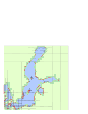
Figure 10: The finest auxiliary grid $\sigma^{(10)}$ contains elements of different size. Left: Dirichlet b.c. ($852$ degrees of freedom), right: Neumann b.c. ($2100$ degrees of freedom)

3.5 Near boundary correction

Since the boundaries of different levels do not coincide, the near boundary error cannot be reduced very well by the standard multigrid method for the Neumann boundary condition. So we introduce a near-boundary region $\Omega_{(\ell,j)}$ where a correction for the boundary approximation will be done. The near-boundary region is defined in layers around the boundary $\Gamma_{\ell}$:

Definition 3 (Near-boundary region).

We define the $j$-th near-boundary region $\mathcal{T}_{(\ell,j)}$ on level $\ell$ of the auxiliary grids by

$$\begin{aligned} \mathcal{T}_{(\ell,0)}:=&\{\tau\in\mathcal{T}_{\ell}\mid{\rm dist}(\Gamma_{\ell},\tau)=0\},\\ \mathcal{T}_{(\ell,i)}:=&\{\tau\in\mathcal{T}_{\ell}\mid{\rm dist}(\mathcal{T}_{(\ell,i-1)},\tau)=0\},\end{aligned}\quad i=1,\ldots,j.$$

The idea for solving the linear system on level $\ell$ is to perform a near-boundary correction after the coarse grid correction. The errors introduced by the coarse grid correction is eliminated by solving the subsystem for the degrees of freedom in the near-boundary region $\mathcal{T}_{(\ell,j)}$. The extra computational complexity is $\mathcal{O}(N)$ because only the elements which are close to the boundary are considered.

Definition 4 (Partition of degrees of freedom).

Let ${{\cal J}}_{\ell}$ denote the index set for the degrees of freedom on the auxiliary grid $\mathcal{T}_{\ell}$. We define the near-boundary degrees of freedom by

$${{\cal J}}_{\ell,j}:=\{i\in{{\cal J}}_{\ell}\mid i\mbox{ belongs to an element }\tau\in\mathcal{T}_{(\ell,j)}\}.$$

Let $(u)_{i\in{{\cal J}}_{\ell}}$ be a coefficient vector on level $\ell$ of the auxiliary grids. Then we extend the standard coarse grid correction by the solve step

$$r^{\ell}:=f-A^{\ell}u^{\ell},\qquad u^{\ell}|_{{\cal J}_{\ell,j}}:=(A^{\ell}|_{{\cal J}_{\ell,j}\times{\cal J}_{\ell,j}})^{-1}r^{\ell}|_{{\cal J}_{\ell,j}}.$$

The small system $A^{\ell}|_{{\cal J}_{\ell,j}}$ of near-boundary elements is solved by an $\cal H$-matrix solver, cf. [25].

Algorithm 3 Auxiliary Space MultiGrid

  For $\ell=0$, define $B_{0}=A_{0}^{-1}$. Assume that $B_{\ell-1}:V_{\ell-1}\rightarrow V_{\ell-1}$ is defined. We shall now define $B_{\ell}:V_{\ell}\rightarrow V_{\ell}$ which is an iterator for the equation of the form

$$A_{\ell}u=f.$$

  Pre-smoothing: For $u^{0}=0$ and $k=1,2,\cdots,\nu$

$$u^{k}=u^{k-1}+R_{\ell}(f-A_{\ell}u^{k-1})$$

  Coarse grid correction: $e_{\ell-1}\in V_{\ell-1}$ is the approximate solution of the residual equation $A_{\ell-1}e=Q_{\ell-1}(f-A_{\ell}u^{\nu})$ by the iterator $B_{\ell-1}$:

$$u^{\nu+1}=u^{\nu}+e_{\ell-1}=u^{\nu}+B_{\ell-1}Q_{\ell-1}(g-A_{\ell}u^{\nu}).$$

  Near boundary correction:

$$u^{\nu+2}=u^{\nu+1}+u^{\ell}|_{{\cal J}_{\ell,j}}=u^{\nu+1}+\left(A^{\ell}|_{{\cal J}_{\ell,j}\times{\cal J}_{\ell,j}}\right)^{-1}(f-A_{\ell}u^{\nu+1})$$

.

  Post-smoothing: For $k=\nu+3,\cdots,2\nu+3$

$$u^{k}=u^{k-1}+R_{\ell}(f-A_{\ell}u^{k-1})$$

4 Convergence of the auxiliary grid method

In this section, we investigate and analyze the new algorithm by verifying the assumptions of the theorem of the auxiliary grid method.

4.1 Overall algorithm

Based on the auxiliary hierarchy we constructed in Section 3, we can define the auxiliary space preconditioner (3) and (9) as follows.

Let the auxiliary space $V=V_{J}$ and $\tilde{A}$ be generated from (2). Since we already have the hierarchy of grids $\{V_{\ell}\}_{\ell=1}^{J}$, we can apply MG on the auxiliary space $V_{J}$ as the preconditioner $\tilde{B}$. On the space $\mathcal{V}$, we can apply a traditional smoother $S$, e.g. Richardson, Jacobi, or Gauß-Seidel. For the stiffness matrix $A=D-L-U$ (diagonal, lower and upper triangular part), the matrix representation of the Jacobi iteration is $S=D^{-1}$ and for the Gauß-Seidel iteration it is $S=(D-L)^{-1}$. (More generally, one could use any smoother that features the spectral equivalence  $\|v\|_{S^{-1}}\mathrel{\hbox{$\hbox{\raise 0.9pt\hbox{$=$}}\kern-7.7778pt\raise-3.5pt\hbox{$\sim$}$}}\parallel h^{-1}v\parallel^{2}_{L^{2}(\Omega)}$.)

The auxiliary grid may be over-refined, it can happen that an element $\tau_{i}\in\mathcal{T}$ intersects much smaller auxiliary elements $\tau^{J}_{j}\in\mathcal{T}_{J}$:

$$\tau_{i}\cap\tau^{J}_{j}\neq\emptyset,\ h_{\tau^{J}_{j}}\lesssim h_{\tau_{i}}\quad\text{but}\quad h_{\tau^{J}_{j}}\not\mathrel{\hbox{$\hbox{\raise 0.9pt\hbox{$=$}}\kern-7.7778pt\raise-3.5pt\hbox{$\sim$}$}}h_{\tau_{i}}.$$ (12)

In this case, we do not have the local approximation and stability properties for the standard nodal interpolation operator. Therefore, we need a stronger interpolation between the original space and the auxiliary space. This is accomplished by the Scott-Zhang quasi-interpolation operator

$$\Pi:H^{1}(\Omega)\rightarrow\mathcal{V}$$

for a triangulation $\mathcal{T}$ [35]. Let $\{\psi_{i}\}$ be an $L^{2}$-dual basis to the nodal basis $\{\varphi_{i}\}$. We define the interpolation operator as

$$\Pi v(x):=\sum_{i\in{\cal J}}\varphi_{i}(x)\int_{\Omega}\psi(\xi)v(\xi)d\xi.$$

By definition, $\Pi$ preserves piecewise linear functions and satisfies (cf. [35]) for all $v\in H^{1}(\Omega)$

$$|\Pi v|^{2}_{1,\Omega}+\sum_{\tau\in\mathcal{T}}h_{\tau}^{-2}\|(v-\Pi v)\|^{2}_{0,\tau}\lesssim|v|^{2}_{1,\Omega}.$$ (13)

We define the new interpolation $\Pi$ from the auxiliary space $V$ to $\mathcal{V}$ by the Scott-Zhang interpolation $\Pi:V\rightarrow\mathcal{V}$ and the reverse interpolation $\tilde{\Pi}:\mathcal{V}\rightarrow V$.

Then we can apply Theorem 1 for $V=V_{J}$. In order to estimate the condition number, we need to verify that the multigrid preconditioner $\tilde{B}$ on the auxiliary space is bounded and the finest auxiliary grid and corresponding FE space we constructed yields a stable and bounded transfer operator and smoothing operator.

4.2 Convergence of the MG on the auxiliary grids

Firstly, we prove the convergence of the multigrid method on the auxiliary space. For the Dirichlet boundary, we have the nestedness

$$\Omega^{D}_{1}\subset\cdots\subset\Omega^{D}_{J}\qquad\subset\Omega,$$

which induces the nestedness of the finite element spaces defined on the auxiliary grids $\mathcal{T}^{D}_{\ell},\ell=1,\cdots,J$:

$$V_{1}\subset V_{2}\subset\cdots\subset V_{J}.$$

In order to avoid overloading the notation, we will skip the superscript $D$ in the following.

In order to prove the convergence of the local multilevel methods by Theorem 3, we only need to verify the assumptions for the decompsition of

$$V_{J}=\sum_{\ell=1}^{J}\sum_{k\in\tilde{N}_{\ell}}V_{\ell,k}.$$ (14)

where

$$\tilde{N}_{\ell}=\{k\in{\cal J}_{\ell}|k\in{\cal J}_{\ell}\setminus{\cal J}_{\ell-1}\text{ or }\varphi_{k,\ell}\neq\varphi_{k,\ell-1}\}.$$

Since $\mathcal{T}_{\ell}\subset\sigma^{(\ell)}$ is the local refinement of $\mathcal{T}_{\ell-1}$, the size of the triangles in $\mathcal{T}_{\ell}$ may be different. We denote $\bar{\cal T}_{\ell}$ as a refinement of the grid ${\cal T}_{\ell}$ where all elements are regularly refined such that all elements from $\bar{\cal T}_{\ell}$ are congruent to the smallest element of ${\cal T}_{\ell}$. The finite element spaces corresponding to $\bar{\cal T}_{\ell}$ are denoted by $\bar{V}_{\ell}$. In the triangulations $\bar{\mathcal{T}}_{\ell}$ we have

$$\tau\in\bar{\mathcal{T}}_{\ell}\quad\Rightarrow\quad h_{\tau}\sim 2^{-\ell}.$$

For an element $\tau\in\mathcal{T}_{\ell}$ we denote by $g_{\tau}$ the level number of the triangulation $\bar{\mathcal{T}}_{g_{\tau}}$ to which $\tau$ belongs, i.e. $h_{\tau}\sim 2^{-g_{\tau}}$. For any vertex $p_{i}$, if $i\in{\cal J}_{\ell}$ but $i\not\in{\cal J}_{\ell-1}$, we define $g_{p_{i}}=\ell$. The following properties about the generation of elements or vertices are [49, 15]

$$\tau\in\bar{\mathcal{T}}_{\ell},\text{ if and only if }g_{\tau}=\ell;$$

$$i\in{\cal J}_{\ell},\text{ if and only if }g_{p_{i}}\leq\ell;$$

$$\text{For }\tau\in\bar{\mathcal{T}}_{\ell},\max_{i\in{\cal J}(\tau)}g_{p_{i}}=\ell=g_{\tau},$$

where ${\cal J}(\tau)$ is the set of vertices of $\tau\in\bar{\mathcal{T}}_{\ell}$.

With the space decomposition (14), we can verify the assumptions of Theorem 3.

4.2.1 Stable decomposition: Proof of (A1)

The purpose of this subsection is to prove the decomposition is stable.

Theorem 4.

For any $v\in V$, there exist function $v^{\ell}_{i}\in V_{\ell,i},i\in\tilde{N}_{\ell}$, $\ell=1,\ldots,J$, such that

$$v=\sum_{\ell=1}^{J}\sum_{i\in\tilde{N}_{\ell}}v^{\ell}_{i}\quad\text{and}\quad\sum_{\ell=1}^{J}\sum_{i\in\tilde{N}_{\ell}}\|v^{\ell}_{i}\|^{2}_{A}\lesssim\log(N)\|v\|^{2}_{A}.$$ (15)

Proof.

Following the argument of [49, 15], we define the Scott-Zhang interpolation between different levels $\Pi_{\ell}:V_{\ell+1}\rightarrow V_{\ell}$, $\Pi_{L}:V_{L}\rightarrow V_{L}$, and $\Pi_{0}:V_{1}\rightarrow 0$.

By the definition, we can define the decomposition as

$$v=\sum_{\ell=1}^{J}v^{\ell},\quad v^{\ell}=(\Pi_{\ell}-\Pi_{\ell-1})v\in V_{\ell}.$$

Assume $v^{\ell}=\sum_{i\in{\cal J}_{\ell}}\xi_{\ell,i}\varphi^{\ell}_{i}$, where $v^{\ell}_{i}=\xi_{\ell,i}\varphi^{\ell}_{i}\in V_{\ell,i}$. Then,

$$\|v^{\ell}_{i}\|^{2}_{0}=\|v^{\ell}_{i}\|^{2}_{0,\omega^{\ell}_{i}}\lesssim\sum_{\tau\in\omega^{\ell}_{i}}h^{d}_{\tau}|v^{\ell}(p_{i})|^{2}\lesssim\|v^{\ell}\|^{2}_{0,\omega^{\ell}_{i}}=\|(\Pi_{\ell}-\Pi_{\ell-1})v\|^{2}_{0,\omega^{\ell}_{i}}.$$

where $\omega^{\ell}_{i}$ is support of $\varphi^{\ell}_{i}$ and the center vertex is $p_{i}$.

By the inverse inequality, we can conclude

$$\sum_{i\in{\cal J}_{\ell}}\|v^{\ell}_{i}\|^{2}_{A}\lesssim\sum_{i\in{\cal J}_{\ell}}\sum_{\tau\in\omega^{\ell}_{i}}h_{\tau}^{-2}\|v^{\ell}_{i}\|^{2}_{0,\tau}\lesssim\sum_{\tau\in\mathcal{T}_{\ell}}h_{\tau}^{-2}\|(\Pi_{\ell}-\Pi_{\ell-1})v\|^{2}_{0,\tau}.$$

Invoking the approximability and stability and following the same argument of Lemma 6, we have

$$\sum_{\tau\in\mathcal{T}_{\ell}}h_{\tau}^{-2}\|(v-\Pi_{\ell}v)\|^{2}_{0,\tau}\lesssim|v|^{2}_{1,\Omega_{\ell+1}}\quad\text{and}\quad\|\Pi_{\ell}v\|^{2}_{0,\Omega_{\ell}}\lesssim\|v\|^{2}_{0,\Omega_{\ell+1}}.$$

So,

$$\sum_{\tau\in\mathcal{T}_{\ell}}h_{\tau}^{-2}\|(\Pi_{\ell}-\Pi_{\ell-1})v\|^{2}_{0,\tau} =\sum_{\tau\in\mathcal{T}_{\ell}}h_{\tau}^{-2}\|\Pi_{\ell}(I-\Pi_{\ell-1})v\|^{2}_{0,\tau}$$

$$\lesssim\sum_{\tau\in\mathcal{T}_{\ell}}h_{\tau}^{-2}\|(I-\Pi_{\ell-1})v\|^{2}_{0,\omega^{\ell}_{\tau}}\lesssim\sum_{\tau\in\mathcal{T}_{\ell}}h_{\tau}^{-2}\|(I-\Pi_{\ell-1})v\|^{2}_{0,\tilde{\omega}^{\ell}}$$

$$\lesssim\sum_{\tau\in\mathcal{T}_{\ell-1}}h_{\tau}^{-2}\|(I-\Pi_{\ell-1})v\|^{2}_{0,\tau}\lesssim|v|^{2}_{1}.$$

where $\omega^{\ell}_{\tau}$ is the union of the elements in $\mathcal{\ell}$ that intersect with $\tau\in\mathcal{T}_{\ell}$ and $\tilde{\omega}^{\ell}_{\tau}$ is the union of the elements in $\mathcal{T}_{\ell-1}$ that intersect with $\omega^{\ell}_{\tau}$. Therefore,

$$\sum_{\ell=1}^{J}\sum_{i\in\tilde{N}_{\ell}}\|v^{\ell}_{i}\|^{2}_{A}\lesssim\sum_{\ell=1}^{J}\sum_{\tau\in\mathcal{T}_{\ell}}h_{\tau}^{-2}\|(\Pi_{\ell}-\Pi_{\ell-1})v\|^{2}_{0,\tau}\lesssim J|v|^{2}_{1}\lesssim\log(N)|v|^{2}_{1}.$$

∎

4.2.2 Strengthened Cauchy-Schwarz inequality: Proof of (A2)

In this subsection, we establish the strengthened Cauchy-Schwarz inequality for the space decomposition (14). Assuming there is an ordering index set $\Lambda=\{\alpha|\alpha=(\ell_{\alpha},k_{\alpha}),k_{\alpha}\in\tilde{N}_{\ell},\ell_{\alpha}=1,\cdots,J\}$. Define the ordering as follows. For any $\alpha,\beta\in\Lambda$, if $\ell_{\alpha}>\ell_{\beta}$ or $\ell_{\alpha}=\ell_{\beta},k_{\alpha}>k_{\beta}$, then, $\alpha>\beta$. The strengthened Cauchy-Schwarz inequality is given as follows.

Theorem 5.

For any $u_{\alpha}=v^{\ell}_{k}\in V_{\alpha}=V_{\ell,i},v_{\beta}=v^{m}_{j}\in V_{\beta}=V_{m,j},\alpha=(\ell,k),\beta=(m,j)\in\Lambda$, we have

$$\bigg{|}\sum_{\alpha\in\Lambda}\sum_{\beta\in\Lambda,\beta>\alpha}(u_{\alpha},v_{\beta})_{A}\bigg{|}\lesssim\bigg{(}\sum_{\alpha\in\Lambda}\|u_{\alpha}\|^{2}_{A}\bigg{)}^{1/2}\bigg{(}\sum_{\beta\in\Lambda}\|u_{\beta}\|^{2}_{A}\bigg{)}^{1/2}.$$

In order to prove the theorem, we need the following lemma:

Lemma 3 (SCS inequality for quasi-uniform meshes).

For any $u_{i}\in\bar{V}_{i},v_{j}\in\bar{V}_{j}$, we have

$$(u_{i},v_{j})_{1}\lesssim\left(\frac{h_{j}}{h_{i}}\right)^{1/2}|u_{i}|_{1}(h_{j}^{-1}\|v_{j}\|_{0}).$$

The proof of the lemma follows from Lemma 4.26 in [48] and Lemma 4.5 in [49].

Now we can prove the theorem 5.

Proof.

For any $\alpha\in\Lambda$, we denote by

$$n(\alpha)=\{\beta\in\Lambda|\beta>\alpha,\omega_{\beta}\cap\omega_{\alpha}\neq\emptyset\},\quad v_{k}^{\alpha}=\sum_{\beta\in n(\alpha),g_{\beta}=k}v_{\beta}.$$

where $\omega_{\alpha}$ is the support of the $V_{\alpha}$ and $g_{\alpha}=\max_{\tau\in\omega_{\alpha}}g_{\tau}$.

Since, the mesh is a K-mesh, for any $\tau\subset\omega_{\alpha}$, we have

$$(u_{\alpha},v^{\alpha}_{k})_{1,\tau}\lesssim\left(\frac{h_{k}}{h_{g_{\alpha}}}\right)^{1/2}|u_{\alpha}|_{1,\tau}h^{-1}_{k}\|v^{\alpha}_{k}\|_{0,\tau}$$

So,

$$(u_{i},v^{\alpha}_{k})_{1,\omega_{\alpha}} =\sum_{\tau\subset\omega_{i}}(u_{i},v^{\alpha}_{k})_{1,\tau}$$

$$\lesssim\sum_{\tau\subset\omega_{\alpha}}\left(\frac{h_{k}}{h_{g_{\alpha}}}\right)^{1/2}|u_{\alpha}|_{1,\tau}h^{-1}_{k}\|v^{\alpha}_{k}\|_{0,\tau}$$

$$\leq\left(\frac{h_{k}}{h_{g_{\alpha}}}\right)^{1/2}|u_{\alpha}|_{1,\omega_{\alpha}}h^{-1}_{k}\left(\sum_{\beta\in n(\alpha),g_{\beta}=k}\|v_{\beta}\|^{2}_{0,\omega_{\alpha}}\right)^{1/2}.$$

Then fix $u_{\alpha}$ and consider

$$\left|(u_{\alpha},\sum_{\beta\in\Lambda,\beta>\alpha}v_{\beta})_{A}\right| \mathrel{\hbox{$\hbox{\raise 0.9pt\hbox{$=$}}\kern-7.7778pt\raise-3.5pt\hbox{$\sim$}$}}\left|(u_{\alpha},\sum_{\beta\in n(\alpha)}v_{\beta})_{1,\omega_{\alpha}}\right|=\left|(u_{\alpha},\sum_{k=g_{\alpha}}^{J}\sum_{\beta\in n(\alpha)}v_{\beta})_{1,\omega_{\alpha}}\right|$$

$$\lesssim\sum_{k=g_{\alpha}}^{J}|(u_{\alpha},v^{\alpha}_{k})_{1,\omega_{\alpha}}|$$

$$\lesssim\sum_{k=g_{\alpha}}^{J}\left(\frac{h_{k}}{h_{g_{\alpha}}}\right)^{1/2}|u_{\alpha}|_{1,\omega_{\alpha}}h^{-1}_{k}\bigg{(}\sum_{g_{\beta}=k}\|v_{\beta}\|^{2}_{0,\omega_{\alpha}}\bigg{)}^{1/2}$$

We sum up the $u_{\alpha}$ level by level,

$$\sum_{\ell=1}^{J}\sum_{g_{\alpha}=\ell}\left|(u_{\alpha},\sum_{\scriptstyle\beta\in\Lambda\atop\scriptstyle\beta>\alpha}v_{\beta})_{A}\right| \lesssim\sum_{\ell=1}^{J}\sum_{g_{\alpha}=\ell}\left[\sum_{k=\ell}^{J}\left(\frac{h_{k}}{h_{\ell}}\right)^{\frac{1}{2}}|u_{\alpha}|_{1,\omega_{\alpha}}h^{-1}_{k}\bigg{(}\sum_{\scriptstyle\beta\in n(\alpha)\atop\scriptstyle g_{j}=k}\|v_{j}\|^{2}_{0,\omega_{\alpha}}\bigg{)}^{\frac{1}{2}}\right]$$

$$\lesssim\sum_{\ell=1}^{J}\sum_{k=\ell}^{J}\Bigg{(}\frac{h_{k}}{h_{\ell}}\sum_{g_{\alpha}=\ell}|u_{\alpha}|^{2}_{1,\omega_{\alpha}}\Bigg{)}^{\frac{1}{2}}\Bigg{(}h^{-2}_{k}\sum_{g_{\alpha}=\ell}\sum_{\scriptstyle\beta\in n(\alpha)\atop\scriptstyle g_{\beta}=k}\|v_{j}\|^{2}_{0,\omega_{\alpha}}\Bigg{)}^{\frac{1}{2}}$$

$$\lesssim\sum_{\ell=1}^{J}\sum_{k=\ell}^{J}\Bigg{(}\frac{h_{k}}{h_{\ell}}\Bigg{)}^{\frac{1}{2}}\Bigg{(}\sum_{g_{\alpha}=\ell}|u_{\alpha}|^{2}_{1,\omega_{\alpha}}\Bigg{)}^{\frac{1}{2}}\Bigg{(}\sum_{g_{\alpha}=\ell}\sum_{g_{\beta}=k}\frac{h^{2}_{\ell}}{h^{2}_{k}}|v_{\beta}|_{1,\omega_{\alpha}}^{2}\Bigg{)}^{\frac{1}{2}}$$

$$\lesssim\Bigg{(}\sum_{\ell=1}^{J}\sum_{g_{\alpha}=\ell}|u_{\alpha}|^{2}_{1}\Bigg{)}^{\frac{1}{2}}\Bigg{(}\sum_{\ell=1}^{J}\sum_{k=\ell}^{J}\sum_{g_{\alpha}=\ell}\sum_{g_{\beta}=k}\frac{h^{2}_{\ell}}{h^{2}_{k}}|v_{\beta}|_{1,\omega_{\alpha}}^{2}\Bigg{)}^{\frac{1}{2}}$$

$$\lesssim\Bigg{(}\sum_{\ell=1}^{J}\sum_{g_{i}=\ell}\|u_{i}\|^{2}_{A}\Bigg{)}^{\frac{1}{2}}\Bigg{(}\sum_{k=1}^{J}\sum_{\ell=1}^{k}\frac{h^{2}_{\ell}}{h^{2}_{k}}\sum_{g_{\beta}=k}|v_{\beta}|_{1}^{2}\Bigg{)}^{\frac{1}{2}}.$$

$$\lesssim\Bigg{(}\sum_{\ell=1}^{J}\sum_{g_{i}=\ell}\|u_{i}\|^{2}_{A}\Bigg{)}^{\frac{1}{2}}\Bigg{(}\sum_{k=1}^{J}\sum_{g_{\beta}=k}\|v_{\beta}\|_{A}^{2}\Bigg{)}^{\frac{1}{2}}.$$

This gives us the desired estimate. ∎

The Gauß-Seidel method as the smoother means choosing the exact inverse for each of the subspaces $V_{\ell,k}$. Therefore, the assumption of the smoother is satisfied as well. Consequently, we have the uniform convergence of the multigrid method on the auxiliary grid.

Theorem 6.

The multigrid method on the auxiliary grid based on the space decomposition (14) is nearly optimal, the convergence rate is bounded by $1-\frac{1}{1+C\log(N)}$.

4.2.3 Condition number estimation

Now, we estimate condition number of the auxiliary space preconditioner by verifying the assumptions in Theorem 1.

The assumption (4) is the continuity of the smoother $S$. We prove the first assumption in Theorem 1 for the Jacobi and Gauß-Seidel iteration. For the Jacobi method, the square of the energy norm can be computed by summing local contributions from the cells $\tau_{i}$ of the mesh $\mathcal{T}$:

$$\|v\|^{2}_{A} =\|\sum_{i\in{\cal J}}\xi_{i}\varphi_{i}\|^{2}_{A}=a(\sum_{i\in{\cal J}}\xi_{i}\varphi_{i},\sum_{j\in{\cal J}}\xi_{j}\varphi_{j})\quad=\sum_{i\in{\cal J}}\sum_{\omega_{i}\cap\omega_{j}\neq\emptyset}a(\xi_{i}\varphi_{i},\xi_{j}\varphi_{j})$$

$$\leq\sum_{i\in{\cal J}}\sum_{\omega_{i}\cap\omega_{j}\neq\emptyset}\frac{1}{2}(\|\xi_{i}\varphi_{i}\|^{2}_{A}+\|\xi_{j}\varphi_{j}\|^{2}_{A})\quad\leq K\sum_{i\in{\cal J}}\|\xi_{i}\varphi_{i}\|^{2}_{A}\quad=K\langle Dv,v\rangle,$$

where K is the maximal number of non-zeros in a row of A. Thus the choice $c_{s}=K$ fulfills the continuity assumption. The continuity of the Gauß-Seidel method can also be proved.

Lemma 4 (Continuity for Gauß-Seidel).

The stiffness matrix $A=D-L-U$ fulfills

$$\frac{1}{K}\langle(D-L)\xi,\xi\rangle\leq\langle D\xi,\xi\rangle\leq 2\langle(D-L)\xi,\xi\rangle,\quad\xi\in\mathbb{R}^{N}.$$ (16)

In order to prove assumptions (5) and (6) , we need the following lemmas for the transfer operator between $\mathcal{V}$ and $V$.

Lemma 5 (Local stability property).

For any auxiliary space function $v\in\tilde{V}$ and any element $\tau\in\mathcal{T}$, the quasi-interpolation $\Pi$ satisfies

$$|\Pi v|_{k,\tau}\lesssim h_{\tau}^{j-k}|v|_{j,\omega_{\tau}},\qquad j,k\in\{0,1\},$$

where $\omega_{\tau}$ is the union of elements in the auxiliary grid $\mathcal{T}$ that intersect with $\tau$.

Lemma 6.

For any auxiliary element function $v\in V$ the reverse interpolation operator $\tilde{\Pi}$ satisfies

$$\sum_{\tau\in\mathcal{T}}h_{\tau}^{-2}\|(v-\tilde{\Pi}v)\|^{2}_{0,\tau}\lesssim|v|^{2}_{1,\Omega}\quad\text{and}\quad|\tilde{\Pi}v|^{2}_{1,\Omega_{J}}\lesssim|v|^{2}_{1,\Omega}.$$ (17)

Proof.

The proof follows an argument presented in Xu [47]. Let $\hat{\mathcal{T}}$ be the set of the elements in $\mathcal{T}$ which do not intersect with $\partial\Omega_{J}$, i.e.

$$\hat{\mathcal{T}}=\{\tau|\tau\in\mathcal{T},\tau\in\Omega_{J}\tau\cap\partial\Omega_{J}=\emptyset\},\quad\overline{\hat{\Omega}}=\bigcup_{\tau\in\hat{\mathcal{T}}}\bar{\tau}.$$

Then,

$$\sum_{\tau\in\mathcal{T}}h_{\tau}^{-2}\|(v-\tilde{\Pi}v)\|^{2}_{0,\tau}\leq\sum_{\tau\in\hat{\mathcal{T}}}h_{\tau}^{-2}\|(v-\tilde{\Pi}v)\|^{2}_{0,\tau}+\sum_{\tau\in\mathcal{T}\setminus\hat{\mathcal{T}}}h_{\tau}^{-2}\|v\|^{2}_{0,\tau}+\sum_{\tau\in\mathcal{T}\setminus\hat{\mathcal{T}}}h_{\tau}^{-2}\|\tilde{\Pi}v\|^{2}_{0,\tau}.$$

For any element $\tau\in\hat{\mathcal{T}}$, $\omega_{\tau}$ is the union of elements in the auxiliary grid $\mathcal{T}_{J}$ that intersect with $\tau$,

$$h_{\tau}^{-2}\|(v-\tilde{\Pi}v)\|^{2}_{0,\tau}\lesssim\sum_{\tilde{\tau}\subset\omega_{\tau}}h_{\tilde{\tau}}^{-2}\|(v-\tilde{\Pi}v)\|^{2}_{0,\tilde{\tau}}\lesssim|v|^{2}_{1,\omega_{\tau}}$$ (18)

So,

$$\sum_{\tau\in\hat{\mathcal{T}}}h_{\tau}^{-2}\|(v-\tilde{\Pi}v)\|^{2}_{0,\tau}\lesssim\sum_{\tau\in\hat{\mathcal{T}}}|v|^{2}_{1,\omega_{\tau}}\lesssim|v|^{2}_{1,\Omega_{J}}\leq|v|^{2}_{1,\Omega}.$$

By the Poincaré inequality and scaling, if $G^{\eta}$ is a reference square ($d=2$) or a cube ($d=3$) of side length $\eta$, then

$$\eta^{-2}\|w\|^{2}_{0,G^{\eta}}\lesssim\int_{G^{\eta}}|\nabla w|^{2}dx$$

holds for all functions $w$ vanishing on one edge of $G^{\eta}$. For any $\tau\in\mathcal{T}\setminus\hat{\mathcal{T}}$, by covering $\tau$ with subregion which can be mapped onto $G^{\eta_{\tau}},\eta_{\tau}\mathrel{\hbox{$\hbox{\raise 0.9pt\hbox{$=$}}\kern-7.7778pt\raise-3.5pt\hbox{$\sim$}$}}h_{\tau}$, we can conclude that

$$\sum_{\tau\in\mathcal{T}\setminus\hat{\mathcal{T}}}h_{\tau}^{-2}\|w\|^{2}_{0,\tau}\lesssim\sum_{\tau\in\mathcal{T}\setminus\hat{\mathcal{T}}}|w|^{2}_{1,G^{\eta_{\tau}}}\lesssim|w|^{2}_{1,\Omega}.$$

Applying the above estimate with $w=v$ and $w=\tilde{\Pi}v$, one has

$$\sum_{\tau\in\mathcal{T}\setminus\hat{\mathcal{T}}}h_{\tau}^{-2}\|v\|^{2}_{0,\tau}+\sum_{\tau\in\mathcal{T}\setminus\hat{\mathcal{T}}}h_{\tau}^{-2}\|\tilde{\Pi}v\|^{2}_{0,\tau}\lesssim|v|^{2}_{1,\Omega}+|\tilde{\Pi}v|^{2}_{1,\Omega}\lesssim|v|^{2}_{1,\Omega}.$$

For the second inequality,

$$|\tilde{\Pi}v|^{2}_{1,\Omega_{J}}\lesssim|v|^{2}_{1,\Omega_{J}}\lesssim|v|^{2}_{1,\Omega}$$

So, we have the desired estimate. ∎

We can now verify the remaining assumptions of Theorem 1.

Lemma 7.

For any $v\in V_{p}$, we have

$$|\Pi v|_{1,\Omega}\lesssim|v|_{1,\Omega_{J}}.$$

Proof.

By the local stability of $\Pi$,

$$|\Pi v|^{2}_{1,\Omega}=\sum_{\tau\in\mathcal{T}}|\Pi v|^{2}_{1,\tau}\lesssim\sum_{\tau\in\mathcal{T}}|v|^{2}_{1,\omega_{\tau}}\lesssim|v|^{2}_{1,\Omega}=|v|^{2}_{1,\Omega_{J}}$$

The desired estimate then follows. ∎

Lemma 8.

For any $v\in V$, there exists $v_{0}\in V$ and $w\in V_{p}$ such that

$$\|v_{0}\|^{2}_{S^{-1}}+|w|^{2}_{1,\Omega_{p}}\lesssim|v|^{2}_{1,\Omega}.$$

Proof.

For any $v\in V$, let $w:=\tilde{\Pi}v$ and $v_{0}=v-\Pi w$, then

$$\|v_{0}\|^{2}_{S^{-1}}+|w|^{2}_{1,\Omega_{J}} \lesssim\sum_{\tau\in\mathcal{T}}h_{\tau}^{-2}\|v-\Pi w\|^{2}_{0,\tau}+|w|^{2}_{1,\Omega_{J}}$$

$$\leq\sum_{\tau\in\mathcal{T}}h_{\tau}^{-2}\|v-\tilde{\Pi}v\|^{2}_{0,\tau}+\sum_{\tau\in\mathcal{T}}h_{\tau}^{-2}\|w-\Pi w\|^{2}_{0,\tau}+|w|^{2}_{1,\Omega_{J}}$$

$$\lesssim|v|^{2}_{1,\Omega}.$$

∎

Theorem 7.

If the multigrid method on the Dirichlet auxiliary grid is the preconditioner $\tilde{B}$ on the auxiliary space and the ASMG preconditioner defined by (3) or (9), then

$$\kappa(BA)\lesssim log(N).$$

5 Numerical results

The numerical tests in this section are all performed on a SunFire with a $2.8$GHz Opteron processor and sufficient main memory. Although the tests are done using only a single processor with access to all the memory, there might be some undesirable scaling effects when using a large portion of the available memory due to the speed of memory access. Therefore, the timings for larger problems are slightly worse than in theory (memory used and flops counted).

In order to compare our code we need a reference point, and this reference is a straightforward geometric multigrid method on a structured grid, where we do not exploit the structure except for it to be a geometric multigird hierarchy. This means we setup the stiffness matrices as well as prolongation and restriction matrices as one would do on a general grid hierarchy.

5.1 Geometric Multigrid

As a test problem we consider the Poisson equation on the unit square with homogeneous Dirichlet boundary conditions:

$$-\Delta u=f\mbox{ in }\Omega:=[0,1]^{2},\qquad u=0\mbox{ on }\Gamma:=\partial\Omega.$$ (19)

For this domain, it is straight-forward to construct a nested hierarchy of regular grids $\mathcal{T}_{1},\ldots\mathcal{T}_{J}$ and corresponding $P_{1}$ finite element spaces $V_{1}\subset\cdots\subset V_{J}$ with $n_{\ell}:={\rm dim}(V_{\ell})=(2^{\ell}-1)^{2}$. Let $(\varphi_{i}^{\ell})_{i=1}^{n_{\ell}}$ denote a Lagrange basis in $V_{\ell}$.

The geometric multigrid algorithm is presented in Algorithm 2. On each level, a smoothing iteration is required which we take to be symmetric Gauß-Seidel. The timings for the setup of the stiffness matrices $A^{\ell}$ and the prolongation matrices $P^{\ell}$ on level $\ell$ as well as for 10 V-cycles ($\nu:=2$ smoothing steps) of geometric multigrid are given in Table 1.

Table 1: The time in seconds for the setup of the matrices and for ten steps of V-cycle (geometric) multigrid, Algorithm 2.

$\#$dof	Setup of $A,P$	10 V-cycles
$n_{9}=1,050,625$	4.3	5.1
$n_{10}=4,198,401$	26.7	39.7
$n_{11}=16,785,409$	108.8	152.3

From the timings, we observe that the geometric multigrid method (with textbook convergence rates) requires roughly $1$ second per step per million degrees of freedom, i.e., roughly $5-10$ seconds per million degrees of freedom to solve the problem. For smaller problems cacheing effects seem to speed up the calculations.

These results for the geometric multigrid method on a uniform grid are now compared with the ASMG method for the baltic sea mesh with strong local refinement and several inclusions.

5.2 ASMG for the Dirichlet problem

Our solver for the unstructured grid from the baltic sea geometry, cf. Figure 7, is a preconditioned conjugate gradient method (CG) where the preconditioner is ASMG. We iterate until the discretisation error on the finest level of the hierarchy is met. In particular, a nested iteration from the coarsest to the finest level is used to obtain good inital values.

We consider the baltic sea model problem with homogeneous Dirichlet boundary conditions. The storage complexity and timings are shown in Table 2. The auxiliary grid hierarchy and matrices require roughly 3 times more storage than the given (unstructured) grid, and the ASMG-CG solve takes approximately 11 seconds per million degrees of freedom, which is at most two times slower than the geometric multigrid method.

Table 2: The storage complexity in bytes per degree of freedom (auxiliary grids, auxiliary matrices and $\cal H$-solvers) and the solve time in seconds for an ASMG preconditioned cg-iteration.

$\#$dof	aux. storage	storage A	aux. setup	ASMG-cg solve (steps)
$n_{4}=737,933$	509	85	45.2	12.4 (5)
$n_{5}=2,970,149$	351	87	124	40.2 (5)
$n_{6}=11,917,397$	281	87	414	125.9 (5)
$n_{7}=47,743,157$	247	88	1360	544.9 (5)

The convergence rates for the ASMG iteration are given in Figure 11, where we plot the residual reduction factors for the first 50 steps. We observe that the rates on all levels are uniformly bounded away from 1, roughly of the size $0.4$.

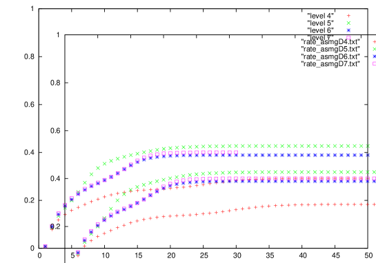
Figure 11: Covergence rates for Auxiliary Space MultiGrid with $n_{4}=737,933$, $n_{5}=2,970,149$, $n_{6}=11,917,397$, and $n_{7}=47,743,157$ degrees of freedom.

5.3 ASMG for the Neumann problem

In the final test, we consider the baltic sea model problem with homogeneous Neumann boundary conditions. Extra near boundary correction has been applied, cf. Algorithm 3. The storage complexity as well as the timing for the ASMG-CG solve are given in Table 3 for the model problem with natural Neumann boundary conditions.

Table 3: The storage complexity in bytes per degree of freedom (auxiliary grids, auxiliary matrices and $\cal H$-solvers) and the solve time in seconds for an ASMG preconditioned cg-iteration.

$\#$dof	aux. storage	aux. setup	storage A	ASMG-cg solve (steps)
$n_{4}=756,317$	355	34.6	88	11.5 (6)
$n_{5}=3,006,917$	244	80	88	33.3 (6)
$n_{6}=11,990,933$	195	266	88	143.6 (6)
$n_{7}=47,890,229$	172	941	88	520.7 (6)

We observe that in order to solve the model problem up to the size of the discretization error, we need to spend twice as much storage for the auxiliary than the given (unstructured) fine grid, and the solve time is roughly 11 seconds per million degrees of freedom.

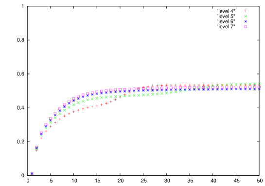
Figure 12: Covergence rates for Auxiliary Space MultiGrid with $n_{4}=756,317$, $n_{5}=3,006,917$, $n_{6}=11,990,933$, and $n_{7}=47,890,229$ degrees of freedom.

In Figure 12 we plot the residual reduction factors for 50 steps of ASMG (without CG acceleration) for 4 consecutive levels. We observe that the rate is level independent and of $0.5$, i.e. bounded away from 1, but not as good as the corresponding rate of the geometric multigrid method.

We conclude that the theoretically proven convergence rates are indeed small enough to be competitive with geometric multigrid in the sense that the storage requirements increase by a factor of at most 3 and the solve times at most by a factor of 2.

References

- [1] Bank, R.E., Dupont, T.: An optimal order process for solving finite element equations. Mathematics of Computation 36(153), 35–51 (1981)
- [2] Bank, R.E., Xu, J.: A hierarchical basis multigrid method for unstructured grids. NOTES ON NUMERICAL FLUID MECHANICS 49, 1–1 (1995)
- [3] Braess, D.: Towards algebraic multigrid for elliptic problems of second order. Computing 55(4), 379–393 (1995)
- [4] Braess, D., Hackbusch, W.: A new convergence proof for the multigrid method including the v-cycle. SIAM Journal on Numerical Analysis 20(5), 967–975 (1983)
- [5] Bramble, J.H., Pasciak, J.E.: New convergence estimates for multigrid algorithms. Mathematics of computation 49(180), 311–329 (1987)
- [6] Bramble, J.H., Pasciak, J.E., Wang, J.P., Xu, J.: Convergence estimates for multigrid algorithms without regularity assumptions. Mathematics of Computation 57(195), 23–45 (1991)
- [7] Bramble, J.H., Pasciak, J.E., Xu, J.: Parallel multilevel preconditioners. Mathematics of Computation 55(191), 1–22 (1990)
- [8] Bramble, J.H., Pasciak, J.E., Xu, J.: The analysis of multigrid algorithms with nonnested spaces or noninherited quadratic forms. Mathematics of Computation 56(193), 1–34 (1991)
- [9] Brandt, A., McCormick, S., Ruge, J.: Algebraic multigrid (AMG) for sparse matrix equations. In: Sparsity and its Applications, pp. 257–284. Cambridge University Press (1984)
- [10] Brandt, A., McCormick, S., Ruge, J.: Algebraic multigrid (AMG) for sparse matrix equations. in Sparsity and Its Applications, edited by Evans, D. pp. 257–284 (1984)
- [11] Brannick, J., Chen, Y., Hu, X., Zikatanov, L.: Parallel unsmoothed aggregation algebraic multigrid algorithms on gpus. In: Numerical Solution of Partial Differential Equations: Theory, Algorithms, and Their Applications, pp. 81–102. Springer (2013)
- [12] Brezina, M., Falgout, R., MacLachlan, S., Manteuffel, T., McCormick, S., Ruge, J.: Adaptive smoothed aggregation (SA) multigrid. SIAM Review 47(2), 317–346 (2005)
- [13] Brezina, M., Vaněk, P., Vassilevski, P.S.: An improved convergence analysis of smoothed aggregation algebraic multigrid. Numerical Linear Algebra with Applications 19(3), 441–469 (2012)
- [14] Bulgakov, V.: Multi-level iterative technique and aggregation concept with semi-analytical preconditioning for solving boundary-value problems. Communications in Numerical Methods in Engineering 9(8), 649–657 (1993)
- [15] Chen, L., Nochetto, R., Xu, J.: Optimal multilevel methods for graded bisection grids. Numerische Mathematik 120(1), 1–34 (2012)
- [16] Chen, L., Zhang, C.: A coarsening algorithm on adaptive grids by newest vertex bisection and its applications. J. Comput. Math 28(6), 767–789 (2010)
- [17] Ciarlet, P.: Basic error estimates for elliptic problems. In: P. Ciarlet and J.-L. Lions, eds., Handbook of Numerical Analysis, Volume II, pp. 17–352. North Holland (1991)
- [18] Falgout, R.D., Vassilevski, P.S.: On generalizing the algebraic multigrid framework. SIAM Journal on Numerical Analysis 42(4), 1669–1693 (2004)
- [19] Falgout, R.D., Vassilevski, P.S., Zikatanov, L.T.: On two-grid convergence estimates. Numerical linear algebra with applications 12(5-6), 471–494 (2005)
- [20] Feuchter, D., Heppner, I., Sauter, S., Wittum, G.: Bridging the gap between ge- ometric and algebraic multigrid methods. Computing and visualization in science 6, 1–13 (2003)
- [21] Feuchter, D., Heppner, I., Sauter, S., Wittum, G.: Bridging the gap between geometric and algebraic multi-grid methods. Computing and visualization in science 6(1), 1–13 (2003)
- [22] Finkel, R., Bentley, J.: Quad trees a data structure for retrieval on composite keys. Acta Informatica 4(1), 1–9 (1974)
- [23] Grasedyck, L., Hackbusch, W., Le Borne, S.: Adaptive geometrically balanced clustering of -matrices. Computing 73, 1–23 (2003)
- [24] Grasedyck, L., Hackbusch, W., LeBorne, S.: Adaptive refinement and clustering of -matrices. Tech. Rep. 106, Max Planck Institute of Mathematics in the Sciences (2001)
- [25] Grasedyck, L., Kriemann, R., LeBorne, S.: Domain-decomposition based -matrix preconditioners. In: Proceedings of DD16, LNSCE. Springer-Verlag Berlin (2005). To appear
- [26] Hackbusch, W.: Multi-grid methods and applications, vol. 4. Springer-Verlag Berlin (1985)
- [27] Henson, V., Yang, U.: BoomerAMG: A parallel algebraic multigrid solver and preconditioner. Applied Numerical Mathematics 41(1), 155–177 (2002)
- [28] Hu, X., Xu, J., Zhang, C.: Application of auxiliary space preconditioning in field-scale reservoir simulation. Science China Mathematics pp. 1–15 (2013)
- [29] Hu, X., Zhang, C.S., Wu, S., , Zhang, S., Wu, X., Xu, J., Zikatanov, L.: Combined preconditioning with applications in reservoir simulation. Multiscale Modeling and Simulation 11(2), 507 – 521 (2013)
- [30] Jones, J., Vassilevski, P.: AMGe based on element agglomeration. SIAM Journal on Scientific Computing 23(1), 109–133 (2002)
- [31] Lashuk, I., Vassilevski, P.: On some versions of the element agglomeration AMGe method. Numerical Linear Algebra with Applications 15(7), 595–620 (2008)
- [32] Liehr, F., Preusser, T., Rumpf, M., Sauter, S., Schwen, L.: Composite finite elements for 3D image based computing. Computing and Visualization in Science 12, 171–188 (2009)
- [33] Nepomnyaschikh, S.: Decomposition and fictitious domains methods for elliptic boundary value problems. In: Fifth International Symposium on Domain Decomposition Methods for Partial Differential Equations, pp. 62–72 (1992)
- [34] Ruge, R.W., Stüben, K.: Efficient solution of finite difference and finite element equations by algebraic multigrid (AMG). In: H.H. D. J. Paddon (ed.) Multigrid Methods for Integral and Differential Equations, pp. 169–212. Clarenden Press Oxford (1985)
- [35] Scott, L.R., Zhang, S.: Finite element interpolation of nonsmooth functions satisfying boundary conditions. Mathematics of computation 54(190), 483–493 (1990)
- [36] Stüben, K.: Algebraic multigrid (AMG): experiences and comparisons. Applied Mathematics and Computation 13(3-4), 419–451 (1983)
- [37] Stüben, K.: Algebraic multigrid (AMG): an introduction with applications. in: U. Trottenberg, C.W. Oosterlee, A. Schüller (Eds.), Multigrid, Academic Press, New York, 2000. Also GMD Report 53, March 1999. (1999)
- [38] Stüben, K.: A review of algebraic multigrid. Journal of Computational and Applied Mathematics 128(1), 281–309 (2001)
- [39] Thum, P., Diersch, H.J., Gründler, R.: SAMG – The linear solver for groundwater simulation. In: MODELCARE 2011. Leipzig, Germany (2011)
- [40] Vaněk, P.: Acceleration of convergence of a two-level algorithm by smoothing transfer operators. Applications of Mathematics 37(4), 265–274 (1992)
- [41] Vaněk, P.: Fast multigrid solver. Applications of Mathematics 40(1), 1–20 (1995)
- [42] Vanek, P., Mandel, J., Brezina, M.: Algebraic multigrid on unstructured meshes, vol. 34. UCD/CCM Report (1994)
- [43] Vaněk, P., Mandel, J., Brezina, M.: Algebraic multigrid by smoothed aggregation for second and fourth order elliptic problems. Computing 56(3), 179–196 (1996)
- [44] Wang, L., Hu, X., Cohen, J., Xu, J.: A parallel auxiliary grid algebraic multigrid method for graphic processing units. SIAM Journal on Scientific Computing 35(3), C263–C283 (2013)
- [45] Xu, J.: Theory of multilevel methods, vol. 8924558. Cornell Unversity, May (1989)
- [46] Xu, J.: Iterative methods by space decomposition and subspace correction. SIAM Review 34(4), 581–613 (1992)
- [47] Xu, J.: The auxiliary space method and optimal multigrid preconditioning techniques for unstructured grids. Computing 56, 215–235 (1996)
- [48] Xu, J.: An introduction to multigrid convergence theory. In: R. Chan, T. Chan, G. Golub (eds.) Iterative Methods in Scientific Computing. Springer-Verlag (1997)
- [49] Xu, J., Chen, L., Nochetto, R.H.: Optimal multilevel methods for , , and systems on graded and unstructured grids. In: R. DeVore, A. Kunoth (eds.) Multiscale, Nonlinear and Adaptive Approximation, pp. 599–659. Springer Berlin Heidelberg (2009)
- [50] Xu, J., Zikatanov, L.: The method of alternating projections and the method of subspace corrections in Hilbert space. Journal of the American Mathematical Society 15(3), 573–597 (2002)
- [51] Yserentant, H.: On the multi-level splitting of finite element spaces. Numerische Mathematik 49(4), 379–412 (1986)
- [52] Yserentant, H.: Old and new convergence proofs for multigrid methods. Acta numerica 2, 285–326 (1993)