Dissociation and dissociative ionization of ${\text{H}_{2}}^{+}$ using the time-dependent surface flux method

Abstract

The time-dependent surface flux method developed for the description of electronic spectra [L. Tao and A. Scrinzi, New J. Phys. 14, 013021 (2012); A. Scrinzi, New J. Phys. 14, 085008 (2012)] is extended to treat dissociation and dissociative ionization processes of ${\text{H}_{2}}^{+}$ interacting with strong laser pulses. By dividing the simulation volume into proper spatial regions associated with the individual reaction channels and monitoring the probability flux, the joint energy spectrum for the dissociative ionization process and the energy spectrum for dissociation is obtained. The methodology is illustrated by solving the time-dependent Schrödinger equation (TDSE) for a collinear one-dimensional model of ${\text{H}_{2}}^{+}$ with electronic and nuclear motions treated exactly and validated by comparison with published results for dissociative ionization. The results for dissociation are qualitatively explained by analysis based on dressed diabatic Floquet potential energy curves, and the method is used to investigate the breakdown of the two-surface model.

I Introduction

The advent of new extreme ultraviolet sources with femtosecond or subfemtosecond duration Sansone et al. (2011); McNeil and Thompson (2010) has sparked interest in measuring the dynamics of atoms and molecules on their natural time scales Krausz and Ivanov (2009). Typically, to obtain time-resolved information, pump-probe schemes have been used, where a pump pulse induces dynamics in the system under investigation and a subsequent probe pulse is applied after a fixed time delay to extract time information. Realizations of such pump-probe methodologies in the subfemtosecond time regime include attosecond streaking spectroscopy Kienberger et al. (2002); Itatani et al. (2002); Schultze et al. (2010) and attosecond interferometry Remetter et al. (2006); Klünder et al. (2011), and these schemes involve couplings to at least a single continuum, which from a theoretical and computational standpoint is challenging due to the requirement of an accurate description of the continua. Extraction of the relevant observables such as the correlated momentum or energy distributions of the final fragments introduces another numerical obstacle. One method is to wait until the bound and scattered parts of the wave function are separated, whereafter a projection of the scattered part onto asymptotic channel eigenstates is performed Laulan and Bachau (2004); Feist et al. (2008); Madsen et al. (2007). This puts a lower limit on the size of the simulation volumes as the scattered part of the wave function must not reach the volume boundaries. Depending on field parameters, this usually requires a huge simulation volume, which is computationally challenging. Another method is to project the total wave function onto exact scattering states at the end of the time-dependent pertubation Fernández and Madsen (2009). The advantage of this is that a smaller simulation volume can be used compared to the former method, while the drawback is the difficulty in obtaining the exact scattering states for a single continuum and the nonexistence of exact scattering states for several continua.

Recently, the time-dependent surface flux (t-SURFF) method Tao and Scrinzi (2012); Scrinzi (2012) was introduced to extract fully differential ionization spectra of one- and two-electron atomic systems from numerical time-dependent Schrödinger equation (TDSE) TDSE calculations. By placing absorbers at the grid boundaries that absorbed the outgoing electron flux, the total number of discretization points used was decreased, thereby reducing the numerical effort. Energy spectra are still obtainable by monitoring the flux passing through surfaces placed at distances smaller than the absorber regions. Several related flux methods already exist, e.g., the “virtual detector” method Feuerstein and Thumm (2003a) and the wave-function splitting technique Keller (1995); Chelkowski et al. (1998). The advantage of the t-SURFF method is that complete information in a given reaction channel can be obtained.

The aim of this work is to demonstrate that the t-SURFF method can be extended to treat molecular systems interacting with a laser field, including both the electronic and nuclear degrees of freedom. The simplest molecule, ${\text{H}_{2}}^{+}$, is of particular interest to physicists, since understanding the fundamental physical processes in this molecule will add valuable insight into more complex molecular systems. There has been impressive experimental and theoretical progress over the past decades in the understanding of laser-induced dissociation and dissociative ionization (DI) phenomena in H${}_{2}^{+}$ Posthumus (2004); Giusti-Suzor et al. (1995). The phenomena described include charge-resonance enhanced ionization Zuo and Bandrauk (1995), bond softening Bucksbaum et al. (1990), bond hardening Yao and Chu (1992, 1993), above-threshold dissociation (ATD) Jolicard and Atabek (1992); Giusti-Suzor et al. (1990), high-order-harmonic generation Zuo et al. (1993), and above-threshold Coulomb explosion Esry et al. (2006).

Much of the insight in these processes comes from calculations involving exact numerical propagation of the TDSE for ${\text{H}_{2}}^{+}$ model systems with reduced dimensionality Kulander et al. (1996); Chelkowski et al. (1998); Feuerstein and Thumm (2003b); Takemoto and Becker (2010); Madsen et al. (2012); Silva et al. (2013); Steeg et al. (2003); Qu et al. (2001). For ${\text{H}_{2}}^{+}$ interacting with a laser pulse, one of the essential questions is how the energy of the pulse is distributed between the resulting fragments. For the DI process, the desired observable is the joint energy spectrum (JES), which displays the differential probability for simultaneously detecting a particular electronic kinetic energy and a particular nuclear kinetic energy Madsen et al. (2012). The JES for DI of H₂ has been considered theoretically in the single-photon ionization regime  González-Castrillo et al. (2012); Silva et al. (2012) and experimentally in the multiphoton regime Wu et al. (2013). Theoretically, the JES of ${\text{H}_{2}}^{+}$ was obtained from numerical TDSE calculations by projecting on approximate double continuum eigenstates at the end of the pulse Madsen et al. (2012), and by using a resolvent technique Silva et al. (2013). In both theoretical works the TDSE was solved on a large numerical grid with many discretization points to ensure that the DI wave packet did not reach the grid boundaries during the pulse duration. For longer pulses, the increase in the discretization points can make the computational effort unmanageable.

The t-SURFF method, when applied to ${\text{H}_{2}}^{+}$, circumvents the before-mentioned deficiencies, and can be used to obtain complete information in a given reaction channel. Hence, not only is it possible to obtain the total nuclear kinetic energy release (KER) spectra for dissociation and DI, the JES for DI and the KER spectrum in each electronic dissociation channel can be obtained as well. Furthermore, the t-SURFF method is extendable to systems with more degrees of freedom, due to the usage of small simulation volumes, and circumvents also in this case the construction of scattering states to extract observables. This makes the t-SURFF method attractive for the study of the laser-induced time-dependent laser-molecule interaction.

The paper is organized as follows. In Sec. II, the ${\text{H}_{2}}^{+}$ model system and the electromagnetic field is described. In Sec. III, the t-SURFF method for ${\text{H}_{2}}^{+}$ is explained. In Sec. IV, the kinetic energy spectra for dissociation and DI from TDSE calculations are obtained for different field parameters. For the DI process, the JES are obtained, while for the dissociation process, the KER for dissociation into H($n=1$) and H($n=2$) are obtained. The concluding remarks are contained in Sec. V. Atomic units are used throughout, unless indicated otherwise.

II Model for ${\text{H}_{2}}^{+}$

To reduce the numerical effort, a simplified model with reduced dimensionality of ${\text{H}_{2}}^{+}$ is employed that includes only the dimension that is aligned with the linearly polarized laser pulse. Within this model, electronic and nuclear degrees of freedom are treated exactly. Such models have been used extensively in the literature and reproduce experimental results at least qualitatively Kulander et al. (1996); Steeg et al. (2003); Qu et al. (2001).

After separating out the center of mass motion of the nuclei, the TDSE for the model ${\text{H}_{2}}^{+}$ molecule in the dipole approximation and velocity gauge reads

$$i\partial_{t}\bigl{|}\Psi(t)\bigr{>}=H(t)\bigl{|}\Psi(t)\bigr{>}$$ (1)

with the Hamiltonian

$$H(t)=T_{\text{e}}+T_{\text{N}}+V_{\text{eN}}+V_{\text{N}}+V_{\text{I}}(t),$$ (2)

where $\bigl{|}\Psi(t)\bigr{>}$ in position space depends on the internuclear distance $R$ and the electronic coordinate $x$ measured with respect to the center-of-mass of the nuclei. The components of the Hamiltonian in Eq. (2) are $T_{\text{e}}=-(1/2\mu)\partial^{2}/\partial x^{2}$, $T_{\text{N}}=-(1/m_{\text{p}})\partial^{2}/\partial R^{2}$, $V_{\text{eN}}=-1/\sqrt{{(x-R/2)^{2}+a(R)}}-1/\sqrt{(x+R/2)^{2}+a(R)}$, $V_{\text{N}}=1/R$, and $V_{\text{I}}(t)=-i\beta A(t)\partial/\partial x$, where $m_{\text{p}}=1.836\times 10^{3}$ a.u. is the proton mass, $\mu=2m_{\text{p}}/(2m_{\text{p}}+1)$ is the reduced electron mass, $\beta=(m_{\text{p}}+1)/m_{\text{p}}$, and the softening parameter $a(R)$ for the Coulomb singularity is chosen to produce the exact three-dimensional $1s\sigma_{g}$ Born-Oppenheimer (BO) potential energy curve Madsen et al. (2012).

The vector potential that we use is of the form

$$A(t)=A_{0}\sin^{2}\left(\frac{\pi t}{T_{\text{pulse}}}\right)\cos(\omega t),$$ (3)

with the angular frequency $\omega$, and the pulse duration $T_{\text{pulse}}$ related to the number of optical cycles $N_{\text{c}}$ by $T_{\text{pulse}}=N_{\text{c}}2\pi/\omega$. The amplitude $A_{0}$ is chosen such that $\omega^{2}A_{0}^{2}=I$, with $I$ the intensity. In this work, we consider laser intensities in the range $I=10^{13}$-$10^{14}$ W/cm², laser frequencies of $400$ and $800$ nm, and the number of optical cycles $N_{\text{c}}=10$.

Equation (1) is solved exactly on a two-dimensional spatial grid using the split-operator, fast Fourier transform (FFT) method Feit et al. (1982), with a time step of $\Delta t=0.005$ in the time propagation. The grid size is defined by $\left|x\right|\leq 100$ and $R\leq 40$, with grid spacings $\Delta x=0.781$ and $\Delta R=0.078$. Complex absorbing potentials (CAPs) are used to absorb the outgoing flux and to avoid reflections at the grid boundaries. Indeed, it is the introduction of the CAP that allows us to use a grid size that is numerically manageable. The form of the CAP is Muga et al. (2004)

$$V_{\text{CAP}}(r)=\begin{cases}-i\eta\left(\left|r\right|-r_{\text{CAP}}\right)^{n}&,|r|\geq r_{\text{CAP}}\\ 0&,\text{elsewhere}\end{cases}$$ (4)

with $r$ being either the electronic coordinate $x$ or the nuclear coordinate $R$. We use $\eta_{e}=0.001$, $x_{\text{CAP}}=55$, and $n_{e}=2$ for the electronic CAP, and $\eta_{N}=0.01$, $R_{\text{CAP}}=26$ and $n_{N}=2$ for the nuclear CAP.

The size of the simulation volume used should be compared with the sizes of the volumes used by other methods. Two other methods have been used to determine the JES based on wave-packet propagation. In one work Madsen et al. (2012), a projection on approximate scattering states was performed and a grid with $\left|x\right|\leq 1500$ was used for the electronic coordinate. In another work Silva et al. (2013), a resolvent technique was used and a grid with $\left|x\right|\leq 3000$ was used for the electronic coordinate. Both these values significantly exceed the size of $\left|x\right|\leq 100$ used here.

III t-SURFF for ${\text{H}_{2}}^{+}$

The t-SURFF method for DI and dissociation is now outlined for the model ${\text{H}_{2}}^{+}$ molecule. For ${\text{H}_{2}}^{+}$ interacting with a laser pulse, there are two continuum channels:

(1) The DI channel ${\text{H}_{2}}^{+}\rightarrow p+p+e$, where the final asymptotic state consists of two protons and one electron separated by large distances. The observable of interest is the JES that shows the energy sharing between the protons and the electron. From the JES, the electronic above-threshold ionization (ATI) and the nuclear KER spectra are obtained by integrating out the appropriate degrees of freedom.

(2) The dissociation channel ${\text{H}_{2}}^{+}\rightarrow\text{H}+p$, where ${\text{H}_{2}}^{+}$ dissociates into a proton and a hydrogen atom in a given state (channel) . The relevant observables are the channel-specific KER spectra that show how the nuclear kinetic energies are shared between the different dissociation channels.

To identify the different channels and the corresponding observables, we partition the total coordinate space into four regions as shown in Fig. 1. Each region corresponds to a reaction channel. By monitoring the flux going through the surfaces at $\left|x\right|=x_{\text{s}}$ and $R=R_{\text{s}}$, the JES for DI and the channel-specific KER for dissociation can be constructed.

Figure 1: Illustration showing the four spatial regions used to analyze the wave packet formed by the interaction of ${\text{H}_{2}}^{+}$ with the external laser pulse. The dashed line at $\left|x\right|=x_{\text{s}}$ is a boundary surface beyond which the electron-nuclear interaction $V_{\text{eN}}$ is neglected in the DI channel, while the dashed line at $R=R_{\text{s}}$ is a boundary surface beyond which the nuclear repulsion $V_{\text{N}}$ is neglected. In the t-SURFF method, the flux passing through these surfaces is monitored and used to construct the differential probability amplitudes. In the figure, the projection operators, formed from Eqs. (5a) and (5b), that project on the different spatial regions are given in the corresponding reaction channels.

To proceed formally, we define the projection operators

$$\theta_{\text{e}} =\int dx\theta(\left|x\right|-x_{\textrm{s}})\bigl{|}x\bigr{>}\bigl{<}x\bigr{|},$$ (5a)

$$\theta_{\text{N}} =\int dR\theta(R-R_{\textrm{s}})\bigl{|}R\bigr{>}\bigl{<}R\bigr{|},$$ (5b)

where $x_{\text{s}}$ and $R_{\text{s}}$ are locations of the surfaces beyond which the Coulomb interactions $V_{\text{eN}}$ and $V_{\text{N}}$ are neglected, respectively, and $\theta(x)$ is the Heaviside step function. These projection operators are used to partition the total wave function into the four parts belonging to the different spatial regions of Fig. 1:

$$\bigl{|}\Psi(t)\bigr{>}=\bigl{|}\Psi_{\text{B}}(t)\bigr{>}+\bigl{|}\Psi_{\text{D}}(t)\bigr{>}+\bigl{|}\Psi_{\text{I}}(t)\bigr{>}+\bigl{|}\Psi_{\text{DI}}(t)\bigr{>},$$ (6)

with $\bigl{|}\Psi_{\text{B}}(t)\bigr{>}=(1-\theta_{\text{e}})(1-\theta_{\text{N}})\bigl{|}\Psi(t)\bigr{>}$, $\bigl{|}\Psi_{\text{D}}(t)\bigr{>}=(1-\theta_{\text{e}})\theta_{\text{N}}\bigl{|}\Psi(t)\bigr{>}$, $\bigl{|}\Psi_{\text{I}}(t)\bigr{>}=\theta_{\text{e}}(1-\theta_{\text{N}})\bigl{|}\Psi(t)\bigr{>}$, and $\bigl{|}\Psi_{\text{DI}}(t)\bigr{>}=\theta_{\text{e}}\theta_{\text{N}}\bigl{|}\Psi(t)\bigr{>}$. For sufficiently large times after the end of the laser pulse $T>T_{\text{pulse}}$, the dissociation and DI wave packets will have moved into their specific spatial regions such that $\bigl{|}\Psi_{\text{B}}(T)\bigr{>}$ contains the bound part of the total wave packet, $\bigl{|}\Psi_{\text{D}}(T)\bigr{>}$ contains the dissociative part, and $\bigl{|}\Psi_{\text{DI}}(T)\bigr{>}$ contains the DI part. At time $T$, the wave packet in the spatial region corresponding to ionization $\bigl{|}\Psi_{\text{I}}(T)\bigr{>}=\theta_{\text{e}}(1-\theta_{\text{N}})\bigl{|}\Psi(T)\bigr{>}=0$, as all the ionized parts will have moved into the DI region since the nuclei do not support bound states after the removal of the electron.

III.1 t-SURFF for dissociative ionization

With the partitioning of space and wave functions, we are now ready to consider the formulation of the t-SURFF methodology for the DI channel ${\text{H}_{2}}^{+}\rightarrow p+p+e$. The projected TDSE on the spatial region describing this channel reads (see Fig. 1)

$$i\partial_{t}\bigl{|}\Psi_{\text{DI}}(t)\bigr{>} =H_{\text{DI}}(t)\bigl{|}\Psi(t)\bigr{>},$$ (7)

where we have defined the projected Hamiltonian $H_{\text{DI}}(t)=\theta_{e}\theta_{\text{N}}H(t)=T_{\text{e}}+T_{\text{N}}+V_{\text{I}}(t)$. It is important to notice that $\bigl{|}\Psi(t)\bigr{>}$, not $\bigl{|}\Psi_{\text{DI}}(t)\bigr{>}$, appears on the right-hand side of Eq. (7). This reflects that $H(t)$ does not commute with $\theta_{\text{e}}\theta_{\text{N}}$ for all times $t$.

The TDSE for $H_{\text{DI}}(t)$ is separable in the electronic and nuclear degrees of freedom, with the electronic TDSE given by

$$i\partial_{t}\bigl{|}\phi(t)\bigr{>}=\left[T_{\text{e}}+V_{\text{I}}(t)\right]\bigl{|}\phi(t)\bigr{>},$$ (8)

and the nuclear TDSE given by

$$i\partial_{t}\bigl{|}\chi(t)\bigr{>}=T_{\text{N}}\bigl{|}\chi(t)\bigr{>}.$$ (9)

A complete set of the solutions in position space is formed by the Volkov waves $\phi_{p}(x,t)=\bigl{<}x\vphantom{\phi_{p}(t)}\bigr{|}\bigl{.}\phi_{p}(t)\vphantom{x}\bigr{>}$ with momentum $p$ for the electronic degree of freedom and plane waves $\chi_{k}(R,t)=\bigl{<}R\vphantom{\chi_{k}(t)}\bigr{|}\bigl{.}\chi_{k}(t)\vphantom{R}\bigr{>}$ with momentum $k$ for the nuclear degree of freedom. The explicit forms of these wave functions, with normalizations $\delta(k-k^{\prime})=\bigl{<}\chi_{k}(t)\vphantom{\chi_{k^{\prime}}(t)}\bigr{|}\bigl{.}\chi_{k^{\prime}}(t)\vphantom{\chi_{k}(t)}\bigr{>}$ and $\delta(p-p^{\prime})=\bigl{<}\phi_{p}(t)\vphantom{\phi_{p^{\prime}}(t)}\bigr{|}\bigl{.}\phi_{p^{\prime}}(t)\vphantom{\phi_{p}(t)}\bigr{>}$, are

$$\phi_{p}(x,t) =(2\pi)^{-1/2}\exp{\left[i\left(px-\frac{p^{2}t}{2\mu}-\frac{p}{\mu}\int^{t}A(t^{\prime})dt^{\prime}\right)\right]},$$ (10)

$$\chi_{k}(R,t) =(2\pi)^{-1/2}\exp{\left[i\left(kR-\frac{k^{2}t}{m_{\text{p}}}\right)\right]}.$$ (11)

The wave packet $\bigl{|}\Psi_{\text{DI}}(t)\bigr{>}$ is expanded in the direct product basis of Volkov and plane waves

$$\bigl{|}\Psi_{\text{DI}}(t)\bigr{>}=\theta_{\text{e}}\theta_{\text{N}}\bigl{|}\Psi(t)\bigr{>}=\int dp\int dkb_{p,k}(t)\bigl{|}\phi_{p}(t)\bigr{>}\bigl{|}\chi_{k}(t)\bigr{>},$$ (12)

where

$$b_{p,k}(T)=\bigl{<}\phi_{p}(t)\bigr{|}\bigl{<}\chi_{k}(t)\bigr{|}\theta_{\text{e}}\theta_{\text{N}}\bigl{|}\Psi(t)\bigr{>}$$ (13)

is the differential probability amplitude for measuring an electronic momentum $p$ and a nuclear momentum $k$. The joint momentum spectrum (JMS) reads

$$\frac{\partial^{2}P}{\partial p\partial k}=\left|b_{p,k}(T)\right|^{2}.$$ (14)

The corresponding JES that gives the differential probability for observing a nuclear KER of $E_{\text{N}}=k^{2}/m_{\text{p}}$ and an electron with energy $E_{\text{e}}=p^{2}/2\mu$ is given by

$$\frac{\partial^{2}P}{\partial E_{\text{e}}\partial E_{\text{N}}}=\sum_{\text{sgn}(p)}\frac{m_{\text{p}}\mu}{2\left|p\right|k}\left|b_{p,k}(T)\right|^{2},$$ (15)

where the summation over $\text{sgn}(p)$ refers to the summation of $\pm p$ corresponding to the same $E_{\text{e}}$.

The expression for $b_{p,k}(T)$ is rewritten using Eqs. (7)$-$(9) and the fundamental theorem of analysis. The result reads

$$b_{p,k}(T)=b^{\text{e}}_{p,k}(T)+b^{\text{N}}_{p,k}(T)$$ (16)

with

$$b^{\text{e}}_{p,k}(T)=i\int_{-\infty}^{T}dt\bigl{<}\phi_{p}(t)\bigr{|}\Bigl{[}T_{\text{e}}+V_{\text{I}}(t),\theta_{\text{e}}\Bigr{]}\bigl{<}\chi_{k}(t)\bigr{|}\theta_{\text{N}}\bigl{|}\Psi(t)\bigr{>},$$ (17)

and

$$b^{\text{N}}_{p,k}(T)=i\int_{-\infty}^{T}dt\bigl{<}\chi_{k}(t)\bigr{|}\Bigl{[}T_{\text{N}},\theta_{\text{N}}\Bigr{]}\bigl{<}\phi_{p}(t)\bigr{|}\theta_{\text{e}}\bigl{|}\Psi(t)\bigr{>}.$$ (18)

In Eqs. (17) and (18), the commutators vanish everywhere except at the discontinuity of the step functions. The probability amplitudes can thus be obtained by integrating the time-dependent surface flux. The amplitude $b_{p,k}^{\text{e}}(T)$ is the amplitude corresponding to the flux going from the dissociation region into the DI region (see Fig. 1), while $b_{p,k}^{\text{N}}(T)$ is the amplitude corresponding to the flux going from the ionization region into the DI region. The two amplitudes must be added coherently to obtain the total amplitude for DI. It is, however, possible to choose $R_{\text{s}}$ sufficiently large so that all the flux going into the DI region in Fig. 1 originate from the ionization region, and therefore we can set $b^{\text{e}}_{p,k}(T)=0$. The commutators in Eqs. (17) and (18) can be calculated explicitly, with

$$\Bigl{[}T_{\text{e}}+V_{\text{I}}(t),\theta_{\text{N}}\Bigr{]}= \int dx\bigl{|}x\bigr{>}\left[-\frac{1}{2\mu}\delta^{(1)}(\left|x\right|-x_{\text{s}})-\textrm{sgn}(x)\delta(\left|x\right|-x_{\text{s}})\left(\frac{1}{\mu}\frac{\partial}{\partial x}+i\beta A(t)\right)\right]\bigl{<}x\bigr{|},$$ (19)

and

$$\Bigl{[}T_{\text{N}},\theta_{\text{N}}\Bigr{]}=-\frac{1}{m_{\text{p}}}\int dR\bigl{|}R\bigr{>}\left[\delta^{(1)}(R-R_{\text{s}})+2\delta(R-R_{\text{s}})\frac{\partial}{\partial R}\right]\bigl{<}R\bigr{|},$$ (20)

where $\delta$ and $\delta^{(1)}$ are the Dirac delta function and its first derivative, respectively. After inserting Eq. (20) into Eq. (18), evaluating the resulting integral and collecting terms in Eq. (16), we obtain

$$b_{p,k}(T) =\frac{1}{m_{\text{p}}}\int_{-\infty}^{T}dt\chi_{k}^{*}(R_{\text{s}},t)\left[k-i\frac{\partial}{\partial R}\right]\bigl{<}\phi_{p}(t)\bigr{|}\theta_{\text{e}}\bigl{|}\Psi(t)\bigr{>}\bigg{|}_{R_{\text{s}}}.$$ (21)

To calculate the amplitude of Eq. (LABEL:eq:DI-b2), the matrix element $\bigl{<}\phi_{p}(t)\bigr{|}\theta_{\text{e}}\bigl{|}\Psi(t)\bigr{>}$ must be evaluated at $R_{\text{s}}$. Direct projection of $\theta_{\text{e}}\bigl{|}\Psi(t)\bigr{>}$ on the Volkov waves $\bigl{|}\chi_{p}(t)\bigr{>}$ is not an option as the electronic CAP [Eq. (4)] will absorb part of the wave function at $\left|x\right|>x_{\text{CAP}}>x_{\text{s}}$. To circumvent this problem we expand $\bigl{<}\phi_{p}(t)\bigr{|}\theta_{\text{e}}\bigl{|}\Psi(t)\bigr{>}$ in an arbitrary time- independent basis $\zeta_{m}(R)$,

$$\bigl{<}\phi_{p}(t)\bigr{|}\theta_{\text{e}}\bigl{|}\Psi(t)\bigr{>}=\sum_{m}a_{p,m}(t)\bigl{|}\zeta_{m}\bigr{>}$$ (22)

with $a_{p,m}(t)=\bigl{<}\zeta_{m}\bigr{|}\bigl{<}\phi_{p}(t)\bigr{|}\theta_{\text{e}}\bigl{|}\Psi(t)\bigr{>}$. In our calculations we use a sine basis for $\zeta_{m}$. By taking the time derivative of $a_{p,m}(t)$ and using Eq. (19) to evaluate the resulting commutator, it can be shown that $a_{p,m}(t)$ satisfies

$$\frac{\text{d}}{\text{d}t}{a}_{p,m}(t)=-i\sum_{m^{\prime}}\bigl{<}\zeta_{m}\bigr{|}T_{\text{N}}+V_{\text{N}}\bigl{|}\zeta_{m^{\prime}}\bigr{>}a_{p,m^{\prime}}(t)+f^{+}_{p,m}(t)+f^{-}_{p,m}(t)$$ (23)

with

$$f^{+}_{p,m}(t)=\phi_{p}^{*}(x_{\text{s}},t)\bigg{[}\left(\frac{p}{2\mu}+\beta A(t)\right)-\frac{i}{2\mu}\frac{\partial}{\partial x}\bigg{]}\bigl{<}\zeta_{m}\vphantom{\Psi(t)}\bigr{|}\bigl{.}\Psi(t)\vphantom{\zeta_{m}}\bigr{>}\bigg{|}_{x_{\text{s}}}$$ (24)

and

$$f^{-}_{p,m}(t)=-\phi_{p}^{*}(-x_{\text{s}},t)\bigg{[}\left(\frac{p}{2\mu}+\beta A(t)\right)-\frac{i}{2\mu}\frac{\partial}{\partial x}\bigg{]}\bigl{<}\zeta_{m}\vphantom{\Psi(t)}\bigr{|}\bigl{.}\Psi(t)\vphantom{\zeta_{m}}\bigr{>}\bigg{|}_{-x_{\text{s}}}.$$ (25)

The terms $f^{+}_{p,m}(t)$ and $f^{-}_{p,m}(t)$ can be interpreted as flux terms, counting the flux going through the surfaces at $x=x_{\text{s}}$ and at $x=-x_{\text{s}}$, respectively. Equation (23) can be solved using any of the standard numerical techniques for solving ordinary differential equations; in our calculations we use a fourth-order Runge-Kutta method with time step 0.05. The coefficients $a_{p,m}(t)$ give us information on the wave packet even in regions where the CAP is active ($\left|x\right|>x_{\text{CAP}}>x_{\text{s}}$), as seen in Eq. (22). When describing laser ionization, one of the two terms in $f_{p,m}(t)$ will usually be negligible and can therefore be ignored. For example if $p$ is positive, then $f^{-}$ will be zero since in this case there is no incoming wave at $x=-x_{\text{s}}$.

Inserting Eq. (22) into Eq. (LABEL:eq:DI-b2), we obtain the final expression for $b_{p,k}(T)$ determining the JMS and JES through Eqs. (14) and (15):

$$b_{p,k}(T)=\frac{1}{m_{\text{p}}}\sum_{m}\left[k-i\frac{\partial}{\partial R}\right]\zeta_{m}(R)\bigg{|}_{R_{\text{s}}}\int_{-\infty}^{T}\text{d}t\chi_{k}^{*}(R_{\text{s}},t)a_{p,m}(t).$$ (26)

III.2 t-SURFF for dissociation

Consider now the dissociation process $\text{H}_{2}^{+}\rightarrow\text{H}+p$. The projected TDSE on the region describing dissociation without ionization reads (see Fig. 1)

$$i\partial_{t}\bigl{|}\Psi_{\text{D}}(t)\bigr{>}=H_{\text{D}}(t)\bigl{|}\Psi(t)\bigr{>},$$ (27)

where we have defined the projected Hamiltonian $H_{\text{D}}(t)=(1-\theta_{\text{e}})\theta_{\text{N}}H(t)$. On the right-hand side $\bigl{|}\Psi(t)\bigr{>}$ and not $\bigl{|}\Psi_{\text{D}}(t)\bigr{>}$ appears [see Eq. (7)].

To obtain the dissociation-channel-specific nuclear KER spectrum we define the adiabatic BO basis states $\bigl{|}\phi_{\text{el},i}\bigr{>}$ as the solutions to the electronic time-independent Schrödinger equation with parametric dependence on $R$:

$$\Big{(}T_{\text{e}}+V_{\text{eN}}+V_{\text{N}}\Big{)}\bigl{|}\phi_{\text{el},i}\bigr{>}=E_{\text{el},i}(R)\bigl{|}\phi_{\text{el},i}\bigr{>},$$ (28)

where $E_{\text{el},i}(R)$ is the $i$th electronic potential energy surface in the BO approximation. To ease notation we do not explicitly include the parametric dependence on $R$ in the BO states.

The wave packet $\Psi_{\text{D}}(x,R,t)$ is expanded in the BO basis as

$$\bigl{|}\Psi_{\text{D}}(t)\bigr{>} =(1-\theta_{\text{e}})\theta_{\text{N}}\bigl{|}\Psi(t)\bigr{>}$$ (29)

$$=\int dk\sum_{i}c_{i,k}(t)\bigl{|}\chi_{k}(t)\bigr{>}\bigl{|}\phi_{\text{el},i}(t)\bigr{>},$$

where $\bigl{|}\chi_{k}(t)\bigr{>}$ is a plane wave with momentum $k$ given in Eq. (11), $\bigl{|}\phi_{\text{el},i}(t)\bigr{>}=\bigl{|}\phi_{\text{el},i}\bigr{>}e^{-iE_{\text{el},i}(R)t}$, and

$$c_{i,k}(t)=\bigl{<}\chi_{k}(t)\bigr{|}\bigl{<}\phi_{\text{el},i}(t)\bigr{|}(1-\theta_{\text{e}})\theta_{\text{N}}\bigl{|}\Psi(t)\bigr{>}.$$ (30)

The bra-ket notation used here indicates integration with respect to both the electronic and nuclear degrees of freedom.

In Eq. (29), all the trivial time dependence is included in $\bigl{|}\phi_{\text{el},i}(t)\bigr{>}$ and $\bigl{|}\chi_{k}(t)\bigr{>}$, while the non trivial time dependence due to the external field and flux going from the bound region into the dissociation region of Fig. 1 is included in the expansion coefficients $c_{i,k}(t)$. At time $T>T_{\text{pulse}}$, when all the dissociative parts of the wave packet have moved into the dissociative region, $c_{i,k}(T)$ describes the differential probability amplitude for the electron to be in the bound state $i$ and the nuclear degree of freedom to have momentum $k$.

The expression for $c_{i,k}(T)$ can be written as

$$c_{i,k}(T)=c_{i,k}^{\text{N}}(T)+c_{i,k}^{\text{e}}(T)+c_{i,k}^{\text{I}}(T),$$ (31)

with

$$c_{i,k}^{\text{N}}(T) =i\int_{-\infty}^{T}dt\bigl{<}\chi_{k}(t)\bigr{|}\Bigl{[}T_{\text{N}},\theta_{\text{N}}\Bigr{]}\bigl{<}\phi_{\text{el},i}(t)\bigr{|}(1-\theta_{\text{e}})\bigl{|}\Psi(t)\bigr{>},$$ (32)

$$c_{i,k}^{\text{e}}(T) =i\int_{-\infty}^{T}dt\bigl{<}\phi_{\text{el},i}(t)\bigr{|}\Bigl{[}T_{\text{e}}+V_{\text{eN}}+V_{\text{N}},(1-\theta_{\text{e}})\Bigr{]}\bigl{<}\chi_{k}(t)\bigr{|}\theta_{\text{N}}\bigl{|}\Psi(t)\bigr{>},$$ (33)

$$c_{i,k}^{\text{I}}(T) =-i\int_{-\infty}^{T}dt\bigl{<}\phi_{\text{el},i}(t)\bigr{|}\bigl{<}\chi_{k}(t)\bigr{|}{(1-\theta_{\text{e}})}\theta_{\text{N}}V_{\text{I}}(t)\bigl{|}\Psi(t)\bigr{>}.$$ (34)

In the derivation of Eq. (32), it is assumed that the action of the nuclear kinetic energy operator on the electronic BO states is neglected. This is in accordance with the BO approximation wherein the first- and second-order derivatives of the electronic state with respect to $R$ are neglected.

In Fig. 1, The amplitude $c_{i,k}^{\text{N}}(T)$ corresponds to the flux going from the bound region into the dissociation region through the surface at $R=R_{\text{s}}$, while $c_{i,k}^{\text{e}}(T)$ corresponds to the flux going through the surfaces at $x=\pm x_{\text{s}}$. The amplitude $c_{i,k}^{\text{e}}$ can thus be neglected if the dissociative wave packet never reaches the surface $x=\pm x_{\text{s}}$ at time $T$. In the pure dissociation process, the electron is localized near one of the protons, i.e., along the lines $x=\pm(1/2)R$. The previous condition can thus always be satisfied if we choose $x_{\text{s}}>R_{\text{s}}/2$.

The amplitude $c_{i,k}^{\text{I}}(T)$ in Eq. (34) includes the time-dependent interaction $V_{\text{I}}(t)$. Let $T_{\text{impact}}$ be the instant at which the fastest part of the dissociative wave packet hits the surface $R=R_{\text{s}}$. Then $c_{i,k}^{\text{I}}(T)$ can be neglected as long as $T_{\text{impact}}\geq T_{\text{pulse}}$. This can be seen by rewriting Eq. (34) as

$$c_{i,k}^{\text{I}}(T) =-i\int_{-\infty}^{T}dt\biggl{\{}\bigl{<}\phi_{\text{el},i}(t)\bigr{|}\bigl{<}\chi_{k}(t)\bigr{|}V_{\text{I}}(t){(1-\theta_{\text{e}})}\theta_{\text{N}}\bigl{|}\Psi(t)\bigr{>}\biggr{.}$$ (35)

$$\qquad\qquad+\biggl{.}\bigl{<}\phi_{\text{el},i}(t)\bigr{|}\bigl{<}\chi_{k}(t)\bigr{|}\Bigl{[}(1-\theta_{\text{e}}),V_{\text{I}}(t)\Bigr{]}\theta_{\text{N}}\bigl{|}\Psi(t)\bigr{>}\biggr{\}}$$

with the commutator in the velocity gauge given by

$$\Bigl{[}(1-\theta_{\text{e}}),V_{\text{I}}(t)\Bigr{]}=-i\beta A(t)\int dx\bigl{|}x\bigr{>}\textrm{sgn}(x)\delta(\left|x\right|-x_{\text{s}})\bigl{<}x\bigr{|}.$$ (36)

For $T_{\text{impact}}\geq T_{\text{pulse}}$, both terms in Eq. (35) are zero. The first term is zero because $\bigl{|}\Psi_{\text{D}}(t)\bigr{>}=(1-\theta_{\text{e}})\theta_{\text{N}}\bigl{|}\Psi(t)\bigr{>}=0$ for $t<T_{\text{pulse}}$, while $V_{\text{I}}(t)=0$ for $t>T_{\text{pulse}}$. Similarly, the second term is zero because $\Psi(\pm x_{\text{s}},R,t)=0$. The condition $T_{\text{impact}}\geq T_{\text{pulse}}$ depends on the interaction $V_{\text{I}}(t)$ and can be satisfied by placing the $R_{\text{s}}$ appropriately.

The final expression for $c_{i,k}(T)$ is then, using Eqs. (20) and (31),

$$c_{i,k}(T) =\frac{1}{m_{\text{p}}}\int_{-\infty}^{T}dt\chi_{k}^{*}(R_{\text{s}},t)\left[k-i\frac{\partial}{\partial R}\right]\bigl{<}\phi_{\text{el},i}(t)\bigr{|}(1-\theta_{\text{e}})\bigl{|}\Psi(t)\bigr{>}\bigg{|}_{R_{\text{s}}}.$$ (37)

We see that the differential probability amplitude $c_{i,k}(T)$ can be calculated by monitoring the flux going through the surface $R=R_{\text{s}}$. Moreover, the electronic BO-states $\phi_{\text{el},i}(x;R)$ with parametric dependence on $R$ only has to be calculated at points close to $R_{\text{s}}$, reducing the numerical effort.

The BO states $\bigl{|}\phi_{\text{el},i}\bigr{>},$ $i=0,1,...$ are even for $i$ even, and odd for $i$ odd. For sufficiently large $R$, the states become pairwise degenerate. It is therefore natural to order the states into pairs, each pair consisting of a gerade and an ungerade state, $\phi_{\text{el},i}^{s},$ $i=0,1,...$, with $s=g,u$. In the dissociation process, the differential probability for the nuclei to have a nuclear KER $E_{\textrm{N}}$ and the electron to be in the $i$th electronic state with parity $s$ is therefore given by

$$\frac{\partial P_{i}^{s}}{\partial E_{\text{N}}}=\frac{m_{\text{p}}}{2k}\left|c_{i,k}^{s}\right|^{2},$$ (38)

where the amplitude $c_{i,k}^{s}$ is given in Eq. (37).

III.3 t-SURFF for dissociation — two-surface model

In numerous previous descriptions of the dissociation process of ${\text{H}_{2}}^{+}$, the BO approximation involving only two bound electronic states has been used  Jolicard and Atabek (1992); Giusti-Suzor et al. (1995); Peng et al. (2005); Leth et al. (2009); Thumm et al. (2008); Niederhausen and Thumm (2008); Niederhausen et al. (2012). By making the ansatz $\Psi(x,R,t)=G_{0}(R,t)\phi_{\text{el},0}(x;R)+G_{1}(R,t)\phi_{\text{el},1}(x;R)$ in Eq. (1), where $G_{0}(R,t)$ and $G_{1}(R,t)$ are the nuclear wave functions corresponding to the lowest gerade $\phi_{\text{el},0}(x;R)$ and ungerade $\phi_{\text{el},1}(x;R)$ electronic states, respectively, the TDSE becomes

$$i\begin{pmatrix}\partial_{t}G_{0}(R,t)\\ \partial_{t}G_{1}(R,t)\end{pmatrix}=\begin{pmatrix}-\frac{1}{m_{\text{p}}}\frac{\partial^{2}}{\partial R^{2}}+E_{\text{el},0}(R)&U_{\text{I}}(t)\\ U_{\text{I}}(t)&-\frac{1}{m_{\text{p}}}\frac{\partial^{2}}{\partial R^{2}}+E_{\text{el},1}(R)\end{pmatrix}\begin{pmatrix}G_{0}(R,t)\\ G_{1}(R,t)\end{pmatrix}.$$ (39)

We refer to this model as the two-surface model. Due to the neglect of the excited and continuum electronic states in the ansatz, the TDSE in Eq. (39) is not gauge invariant. The dynamics are only correctly described in the length gauge Giusti-Suzor et al. (1995), where $U_{\text{I}}(t)=\beta_{\textrm{LG}}\bigl{<}\phi_{\text{el},1}(R)\bigr{|}x\bigl{|}\phi_{\text{el},0}(R)\bigr{>}F(t)$, with the electric field $F(t)=-\partial_{t}A(t)$ and $\beta_{\textrm{LG}}=1+1/(2m_{\text{p}}+1)$. Here, we propagate Eq. (39) using the split-operator FFT method of Ref. Schwendner et al. (1997).

The KER spectrum in the two-surface model can also be obtained by the t-SURFF method. The dissociation-channel-specific differential probability amplitudes $c^{\text{2-BO}}_{i,k}(T)$, with $i=0,1$, corresponding to the two BO states, read

$$c^{\text{2-BO}}_{i,k}(T) =\bigl{<}\chi_{k}(T)\bigr{|}\theta_{\text{N}}\bigl{|}G_{i}(T)\bigr{>}$$ (40)

$$=\frac{1}{m_{\text{p}}}\int_{-\infty}^{T}dt\chi_{k}^{*}(R_{\text{s}},t)\left[k-i\frac{\partial}{\partial R}\right]G_{i}(t)\bigg{|}_{R_{\text{s}}},$$

which is obtained using the techniques of the previous two sections. As in Sec. III.2, we have assumed that the laser pulse is over at the time the dissociative wave packet first hits the surface $R_{\text{s}}$. The dissociative spectrum within the two-surface model obtained using t-SURFF was compared with the results in Ref. Jolicard and Atabek (1992) and a perfect match was observed.

IV Results and Discussion

To demonstrate the t-SURFF method for ${\text{H}_{2}}^{+}$, the TDSE of Eq. (1) is solved with ${\text{H}_{2}}^{+}$ initially in the ground state. The ground state is obtained by propagation in imaginary time. Two different sets of laser pulse parameters are used: one set with $\lambda=400\;\text{nm}$, $N_{\text{c}}=10$, and $I=8.8\times 10^{13}$ W/cm²; another with $\lambda=800\;\text{nm}$, $N_{\text{c}}=10$, and $I=8.8\times 10^{13}$ W/cm². For the first pulse the duration is $T_{\text{pulse}}=13.3$ fs, the photon energy is $\omega=3.1$ eV and the Keldysh parameter Keldysh (1964) is $\gamma=3.4$, indicating that the dynamics take place in the multiphoton ionization regime. For the second pulse the duration is $T_{\text{pulse}}=26.7$ fs, $\omega=1.55$ eV, and $\gamma=1.7$, placing the dynamics closer to the tunneling regime. These pulse parameters are chosen to facilitate comparisons with recent calculations using the same model for ${\text{H}_{2}}^{+}$ Madsen et al. (2012); Silva et al. (2013). All the following results are obtained with $x_{\text{s}}=50$ and $R_{\text{s}}=25$. Convergence of all results are checked by performing calculations with varying grid spacings, simulation volumes, CAP parameters, placement of t-SURFF surfaces, and observing that the results match. The convergence with respect to propagation time deserves special mentioning. The time $T$, at which the dissociation and DI wave packets have moved inside their respective regions (see Fig. 1), is written as $T=T_{\textrm{pulse}}+T_{\textrm{free}}$, with $T_{\textrm{free}}$ being the propagation time after the pulse. An estimate of $T_{\textrm{free}}$ for DI can be made by assuming the slowest nuclei to have $E_{N}=1/R_{{\textrm{cl},0}}$, where $R_{{\textrm{cl},0}}$ is the outer classical turning point of the ground vibrational state. An estimate for $T_{\textrm{free}}$ is then given by $R_{\textrm{s}}\sqrt{R_{{\textrm{cl},0}}m_{\textrm{p}}/2}=932$. To obtain a more accurate $T_{\textrm{free}}$ numerical tests are performed, and it is found that choosing $T_{\textrm{free}}=1200$ will lead to the convergence of both the dissociation and the DI spectra.

IV.1 Results for Dissociative ionization

Figure 2 shows the JES spectrum for the DI process of ${\text{H}_{2}}^{+}$ with laser parameters $\lambda=400\;\text{nm}$, $N_{\text{c}}=10$, and $I=8.8\times 10^{13}$ W/cm². We can compare Figure 2 with the results presented in Fig. 1(a) of Ref. Madsen et al. (2012) with the same field parameters and a perfect match is observed. In Ref. Madsen et al. (2012), an electric field $F(t)$ with a sine-squared envelope was used, whereas in the present work the vector potential $A(t)$ has a sine-squared envelope (3). The agreement between the results is expected, as the large $N_{\text{c}}$ value makes the carrier envelope phase difference between the pulses insignificant. In Fig. 2 the energy conservation lines in the JES satisfying $E_{\text{N}}+E_{\text{e}}=E_{0}+n\omega-U_{\text{p}}$ are clearly seen, where $E_{0}=-0.597$ a.u. is the ground state energy of ${\text{H}_{2}}^{+}$ and $U_{\text{p}}=A_{0}^{2}/4=0.0483$ a.u. is the ponderomotive energy.

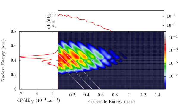
Figure 2: (Color online) JES for DI [Eq. $\eqref{eq:DI-JES}$] for a pulse with parameters $\lambda=400\;\text{nm}$, $N_{\text{c}}=10$, and $I=8.8\times 10^{13}$ W/cm². The top and left side panels are the ATI and nuclear KER spectra, respectively. The diagonal (white) lines are energy conservation lines corresponding to $n$-photon absorption and satisfying $E_{\text{N}}+E_{\text{e}}=E_{0}+n\omega-U_{\text{p}}$, with the leftmost line corresponding to $n=9$.

Figure 3 shows the JES spectrum for the DI process for $\lambda=800\;\text{nm}$, $N_{\text{c}}=10$, and $I=8.8\times 10^{13}$ W/cm². For the part of the JES with $E_{\text{e}}\gtrsim 0.4$ a.u., the energy conservation lines are evident. At low electronic energies ($E_{\text{e}}\lesssim 0.4$ a.u.), the energy conservation lines are not as clear. Instead, interference patterns are seen, corresponding to different pathways leading to the same final double-continuum state. Similar blurring of the photon-absorption lines was reported in Ref. Silva et al. (2013), where the change in the shape of the spectrum was interpreted as a signature of tunneling ionization. Figures 2 and 3 show that the t-SURFF method can be used to describe DI.

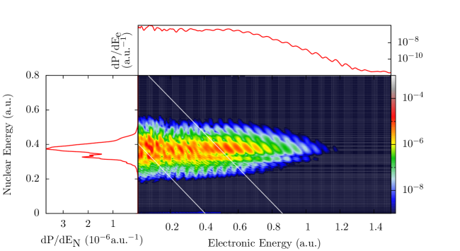
Figure 3: (Color online) Same as Fig. 2, but for $\lambda=800\;\text{nm}$, $N_{\text{c}}=10$, and $I=8.8\times 10^{13}$ W/cm². The diagonal (white) lines are energy conservation lines corresponding to $n$-photon absorption and satisfying $E_{\text{N}}+E_{\text{e}}=E_{0}+n\omega-U_{\text{p}}$. The left diagonal (white) line corresponds to $n=21$, while the right diagonal (white) line corresponds to $n=29$.

IV.2 Results for dissociation

Figure 4(a) shows the nuclear KER spectrum for the 400 nm pulse with dissociation via the two first electronic states $\phi_{\text{el},0}^{g/u}$ corresponding to the $1s\sigma_{g}$ and $2p\sigma_{u}$ states. A comparison of the magnitudes of the probabilities with Fig. 2 shows that dissociation dominates over the DI process for these field parameters, although the DI yield cannot be entirely neglected as done in the two-surface model. The vertical dashed lines in Fig. 4(a) are the $n$-photon energy conservation lines satisfying $E_{0}+n\omega=E_{\text{el},0}(R=\infty)+E_{\text{N}}$, where $E_{\text{el},0}(R=\infty)$ is the ground state energy of the hydrogen atom. Dissociation via $1s\sigma_{g}$ is located around the two-photon line, while dissociation via $2p\sigma_{u}$ is located around the three-photon line. This result can be understood by drawing the diabatic Floquet potential curves Giusti-Suzor et al. (1995); Posthumus (2004), shown in Fig. 5(a).

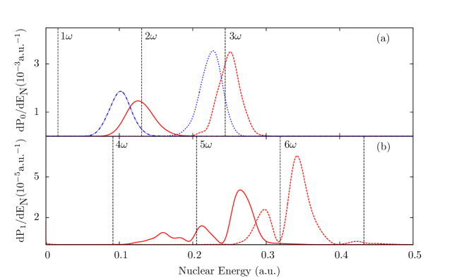
Figure 4: (Color online) Dissociation spectra [Eq. (38)] for a pulse with $\lambda=400\;\text{nm}$, $N_{\text{c}}=10$, and $I=8.8\times 10^{13}$ W/cm² with dissociation via (a) the first pair of gerade/ungerade states ($1s\sigma_{g}$ and $2p\sigma_{u}$), and (b) the second pair of gerade/ ungerade states ($2s\sigma_{g}$ and $3p\sigma_{u}$). The solid (red) and the dashed (red) lines show dissociation via the gerade and ungerade states, respectively, in the TDSE calculation. The dashed- dotted (blue) and the dotted (blue) lines show dissociation via the gerade and ungerade states, respectively, in the two-surface BO calculation, scaled by a factor of 0.13. The vertical lines labeled by $n\omega$ ($n=1,2,\dots,6$) denote photon absorptions above threshold (see text).

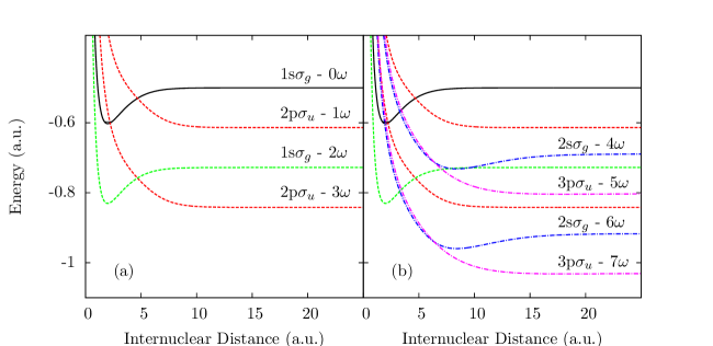
Figure 5: (Color online) The diabatic Floquet potentials for the one-dimensional ${\text{H}_{2}}^{+}$ model with $\lambda=400$nm. (a) Relevant dressed curves of $1s\sigma_{g}$ and $2p\sigma_{u}$ symmetry. (b) Additional dressed curves of $2s\sigma_{g}$ and $3p\sigma_{u}$ symmetry.

Starting from the vibrational ground state, the laser can induce a dissociative wave packet by the ATD process, which will move down the $2p\sigma_{u}-3\omega$ curve. The time for the wave packet to move from the intersection between $1s\sigma_{g}-0\omega$ and $2p\sigma_{u}-3\omega$ at $R=2.23$ a.u. to the intersection between $1s\sigma_{g}-2\omega$ and $2p\sigma_{u}-3\omega$ at $R=4.7$ a.u. is approximately 204 a.u. (4.93 fs). At the latter intersection, part of the population can be transferred to the $1s\sigma_{g}-2\omega$ curve by stimulated photoemission. The time for the population to move from $R=4.7$ to $R=10$ via the surface $1s\sigma_{g}-2\omega$ is approximately 311 a.u. (7.52 fs), so the total time to reach $R=10$ a.u. from the vibrational ground state via the described pathway approximately equals the pulse duration. The pulse duration is therefore not long enough to induce transitions between the $1s\sigma_{g}-2\omega$ and $2p\sigma_{u}-1\omega$ curves, nor is it intense enough to lower the adiabatic Floquet potentials (gap proportional to electric field) to induce tunneling from the vibrational ground state ($v=0$) to the $2p\sigma_{u}-1\omega$ curve. This is the reason for the absence of the one-photon peak in the nuclear KER spectrum.

In addition to the TDSE calculation, a calculation in the BO-approximation is performed for the two-surface model with the lowest pair of electronic states $1s\sigma_{g}$ and $2p\sigma_{u}$. In Fig. 4(a) it is seen that the nuclear KER yield for this model is shifted more from the energy-conservation lines than the TDSE calculation, indicating that the ac-Stark shift is inaccurately accounted for in the two-surface model. Moreover, the dissociation yield is greatly overestimated by the two-surface model, which is understandable as in this model the excited electronic states together with the double continuum are completely neglected. The two-surface model is thus expected to be more accurate for lower laser intensities than for high intensities, where the coupling to the excited states and double continuum is strong.

Figure 4(b) shows the nuclear KER spectrum for the 400 nm pulse with dissociation via the third and fourth electronic states $\phi_{\text{el},1}^{g/u}$ corresponding to the $2s\sigma_{g}$ and $3p\sigma_{u}$ states. The vertical dashed lines in Fig. 4(b) are the $n$-photon energy conservation lines satisfying $E_{0}+n\omega=E_{\text{el},1}(R=\infty)+E_{\text{N}}$, where $E_{\text{el},1}(R=\infty)$ is the energy of the first excited state in hydrogen. Dissociation via $2s\sigma_{g}$ is located between the four- and six-photon lines, while dissociation via $3p\sigma_{u}$ is located between the five- and seven-photon lines.

To understand the dissociation spectrum in Fig. 4(b), the Floquet potential curves for $2s\sigma_{g}$ and $3p\sigma_{u}$ dressed by four to seven photons are plotted in Fig. 5(b). Furthermore, a study is performed where we gradually increase the intensity of the laser field and observe the resulting nuclear KER spectra, shown in Fig. 6. At lower intensities, $I\lesssim 2\times 10^{13}$ W/cm² in Figs. 6(a) and 6(b), the four-photon peak for the gerade state and the five-photon peak for the ungerade state are clearly seen, stemming from the wave packet following the pathway $1s\sigma_{g}-0\omega$ $\rightarrow$ $2p\sigma_{u}-3\omega$ $\rightarrow$ $1\sigma_{g}-2\omega$ $\rightarrow$ $2\sigma_{g}-4\omega$ and $3p\sigma_{u}-5\omega$, shown in Fig. 5(b). This is also indicated by the $2s\sigma_{g}-4\omega$ and $3p\sigma_{u}-5\omega$ curves in Fig.  5(b). In Fig. 6(b) a small peak at around $E_{\text{N}}=0.4$ a.u. is seen for the ungerade state and a smaller peak at around $E_{\text{N}}=0.27$ a.u. is seen for the gerade state. These are the ac-Stark-shifted seven-photon and six-photon absorption peaks, respectively. Figure 5(b) clearly shows that the $3p\sigma_{u}-7\omega$ and $2s\sigma_{g}-6\omega$ curves cross the $1s\sigma_{g}-0\omega$ curve at $R=2$ a.u., below the energy of the vibrational ground state ($v=0$), leading to ATD processes explaining the peaks in Fig. 6(b). As the intensity is increased from Fig. 6(c) to Fig. 6(h), the seven-photon and eight-photon peaks are Stark shifted to lower nuclear energies, and additional structures in the peaks emerge. The additional structures are believed to be due to the interferences from the near degeneracy of the $3p\sigma_{u}-7\omega$ and $2s\sigma_{g}-6\omega$ curves in Fig. 5(b) for $R<7$ a.u., i.e., the strong coupling inducing many one-photon absorption and emission paths that all lead to the same final dissociating state.

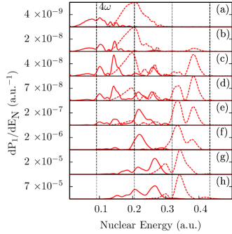
Figure 6: (Color online) Each subplot is as in Fig. 4(b), now for the intensities: (a) $I=1\times 10^{13}$ W/cm², (b) $I=2\times 10^{13}$ W/cm², (c) $I=3\times 10^{13}$ W/cm², (d) $I=3.5\times 10^{13}$ W/cm², (e) $I=4\times 10^{13}$ W/cm², (f) $I=5\times 10^{13}$ W/cm², (g) $I=8\times 10^{13}$ W/cm², and (h) $I=1\times 10^{14}$ W/cm².

Figure 7(a) shows the nuclear KER spectrum for a 10 cycle, 800 nm pulse with dissociation via the two first electronic states $\phi_{\text{el},0}^{g/u}$. Comparing with Fig. 3, we see that the dissociation process is also the most dominant for these field parameters. Dissociation via $1s\sigma_{g}$ is located around the four-photon line, while dissociation via $2p\sigma_{u}$ is located around the five-photon line. This result can be understood by looking at the diabatic Floquet potential curves in Fig. 8(a).

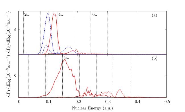
Figure 7: (Color online) Same as Fig. 4, but for a pulse with parameters $\lambda=800\;\text{nm}$, $N_{\text{c}}=10$, and $I=8.8\times 10^{13}$ W/cm².

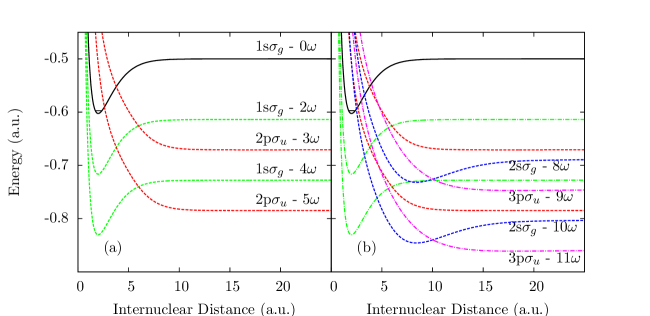
Figure 8: (Color online) Same as Fig. 5, but for a pulse with parameters $\lambda=800\;\text{nm}$, $N_{\text{c}}=10$, and $I=8.8\times 10^{13}$ W/cm².

Starting from the vibrational ground state, coupling to the field can induce a dissociative wave packet on the $2p\sigma_{u}-5\omega$ surface, at a time when the intensity of the pulse is large enough for five-photon absorption. The time for the wave packet to move from the intersection between $1s\sigma_{g}-0\omega$ and $2p\sigma_{u}-5\omega$ at $R=2.61$ a.u. to the intersection between $1s\sigma_{g}-2\omega$ and $2p\sigma_{u}-5\omega$ at $R=3.79$ a.u. is approximately 203 a.u. (4.919 fs). To reach the $1s\sigma_{g}-2\omega$ surface involves the emission of three photons, and the wave packet has therefore a larger probability of continuing along the dissociative $2p\sigma_{u}-5\omega$ surface until it hits the intersection between $2p\sigma_{u}-5\omega$ and $1s\sigma_{g}-4\omega$ at $R=6$ a.u. around 347 a.u. (8.38 fs). The wave packet then moves along the $2p\sigma_{u}-5\omega$ and $1s\sigma_{g}-4\omega$ to asymptotic distances and yields the four- and five-photon peaks in the nuclear KER spectrum of Fig. 7.

Figure 7(b) shows the nuclear KER spectrum for the 800 nm pulse with dissociation via $2s\sigma_{g}$ and $3p\sigma_{u}$. Dissociation via $2s\sigma_{g}$ is seen to be located between the eight-photon and ten-photon lines, while dissociation via $3p\sigma_{u}$ is located between the ten-photon and 13-photon lines. The $2s\sigma_{g}$ peak is due to dissociation after ten-photon absorption, while the $3p\sigma_{u}$ peak is due to dissociation after 11-photon absorption. This is consistent with Fig. 8(b), where the $3p\sigma_{u}-11\omega$ and $2s\sigma_{g}-10\omega$ crossings with the $1s\sigma_{g}-0\omega$ curve are below the energy of the vibrational ground state ($v=0$).

V Conclusion

We extended the t-SURFF method originally introduced for the determination of electronic spectra Tao and Scrinzi (2012); Scrinzi (2012) to extract information from TDSE calculations for dissociation and DI of molecules. Using the example of ${\text{H}_{2}}^{+}$, the JES of DI and the nuclear KER spectrum of the dissociation process were extracted and analyzed. Laser pulses with intensity $8.8\times 10^{13}$ W/cm², ten optical cycles, and wavelengths of $400$ and $800$ nm were used. For the shorter wavelength, the JES exhibited energy conservation lines described by $E_{\text{N}}+E_{\text{e}}=E_{0}+n\omega-U_{\text{p}}$, while for the longer wavelength the conservation lines for electronic energies less than 0.4 a.u. were smeared out due to interference effects. For the dissociation process, the nuclear KER spectra were explained qualitatively by looking at the diabatic Floquet potentials. It was found that the two-surface model, where only the first two electronic states in the BO approximation are taken into account, overestimates the ac-Stark shifts and the dissociation yields. In addition to dissociation via $1s\sigma_{g}$ and $2p\sigma_{u}$, the dissociation spectra via higher excited electronic states $2s\sigma_{g}$ and $3p\sigma_{u}$ were obtained. These spectra were explained qualitatively by observing the gradual change in the nuclear KER spectra as the intensity was scanned from relatively low to high values.

The present work demonstrates that the t-SURFF method is able to describe the break up of ${\text{H}_{2}}^{+}$. The t-SURFF method requires modest spatial simulation volumes, and can be used to determine both photoelectron, KER and joint energy and momentum spectra. The t-SURFF method requires small simulation volumes compared to other standard methods for the extraction of observables. For instance, in our present calculations using t-SURFF, a simulation volume of $\left|x\right|\leq 100$ is used for the electronic coordinate, which is much smaller than $|x|\leq 1500$ Madsen et al. (2012) and $|x|\leq 3000$ Silva et al. (2013) used previously. The simulation volume in the t-SURFF method can be further decreased by improving the complex absorber or implementing the infinite exterior complex scaling method Scrinzi (2010). The relatively small simulation volume makes the method attractive for extension to molecules with more electronic and nuclear degrees of freedom.