Learning Topology and Dynamics of Large Recurrent Neural Networks

Abstract

Large-scale recurrent networks have drawn increasing attention recently because of their capabilities in modeling a large variety of real-world phenomena and physical mechanisms. This paper studies how to identify all authentic connections and estimate system parameters of a recurrent network, given a sequence of node observations. This task becomes extremely challenging in modern network applications, because the available observations are usually very noisy and limited, and the associated dynamical system is strongly nonlinear. By formulating the problem as multivariate sparse sigmoidal regression, we develop simple-to-implement network learning algorithms, with rigorous convergence guarantee in theory, for a variety of sparsity-promoting penalty forms. A quantile variant of progressive recurrent network screening is proposed for efficient computation and allows for direct cardinality control of network topology in estimation. Moreover, we investigate recurrent network stability conditions in Lyapunov’s sense, and integrate such stability constraints into sparse network learning. Experiments show excellent performance of the proposed algorithms in network topology identification and forecasting.

I Introduction

There has been an increasing interest in identifying network dynamics and topologies in the emerging scientific discipline of network science. In a dynamical network, the evolution of a node is controlled not only by itself, but also by other nodes. For example, in gene regulatory networks [1], the expression levels of genes influence each other, following some dynamic rules, such that the genes are connected together to form a dynamical system. If the topology and evolution rules of the network are known, we can analyze the regulation between genes or detect unusual behaviors to help diagnose and cure genetic diseases. Similarly, the modeling and estimation of dynamical networks are of great importance in various domains including stock market, brain network and social network [2, 3, 4]. To accurately identify the topology and dynamics underlying those networks, scientists are devoted to developing appropriate mathematical models and corresponding estimation methods.

In the literature, linear dynamical models are commonly used. For example, the human brain connectivity network [5] can be characterized by a set of linear differential equations, where the rate of change of activation/observation of any node is a weighted sum of the activations/observations of its neighbors: ${\,\mathrm{d}x_{i}}/{\,\mathrm{d}t}=\sum_{j\neq i}\alpha_{ij}x_{j}-d_{i}x_{i},1\leq i\leq n.$ Here $\alpha_{ij}$ provide the connection weights and $d_{i}$ is the decay rate. Nevertheless, a lot of complex dynamical networks clearly demonstrate nonlinear relationships between the nodes. For instance, the strength of influence is unbounded in the previous simple linear combination, but the so-called “saturation” effect widely exists in physical/biological systems (neurons, genes, and stocks)—the external influence on a node, no matter how strong the total input activation is, cannot go beyond a certain threshold. To capture the mechanism, nonlinearity must be introduced into the network system: ${\,\mathrm{d}x_{i}}/{\,\mathrm{d}t}=l_{i}\pi(\sum_{j\neq i}\alpha_{ij}x_{j}+u_{i})-d_{i}x_{i}+c_{i}$, where $\pi$ denotes a nonlinear activation function typically taken to be the sigmoidal function $\pi(\theta)={1}/({1+e^{-\theta}})$. It has a proper shape to resemble many real-world mechanisms and behaviors.

The model description is associated with a continuous-time recurrent neural network. The existing feedback loops allow the network to exhibit interesting dynamic temporal behaviors to capture many kinds of relationships. It is also biologically realistic in say modeling the effect of an input spike train. Recurrent networks have been successfully applied to a wide range of problems in bioinformatics, financial market forecast, electric circuits, computer vision, and robotics; see, e.g., [6, 7, 8, 9, 10] among many others.

In practical applications, it is often necessary to include noise contamination: $\,\mathrm{d}x_{i}=(l_{i}\pi(\sum_{j\neq i}\alpha_{ij}x_{j}+u_{i})-d_{i}x_{i}+c_{i})\,\mathrm{d}t+\sigma\,\mathrm{d}\mathcal{B}_{t},1\leq i\leq n,$ where $\mathcal{B}_{t}$ stands for an $n$-dimensional Brownian motion. Among the very many unknown parameters, $\alpha_{ij}$ might be the most important: the zero-nonzero pattern of $\alpha_{ij}$ indicates if there exists a (direct) connection from node $j$ to node $i$. Collecting all such connections results in a directed graph to describe the node interaction structure.

A fundamental question naturally arises: Given a sequence of node observations (possibly at very few time points), can one identify all existing connections and estimate all system parameters of a recurrent network?

This task becomes extremely challenging in modern big network applications, because the available observations are usually very noisy and only available at a relatively small number of time points (say $T$), due to budget or equipment limitations. One frequently faces applications with $n^{2}$ much larger than $T$. In addition, in this continuous time setting, no analytical formula of the likelihood exists for the stochastic model, which increases the estimation difficulty even in large samples [11]. Instead of considering multi-step ad-hoc procedures, this paper aims at learning the network system as a whole. Multivariate statistical techniques will be developed for identifying complete topology and recovering all dynamical parameters. To the best of our knowledge, automatic topology and dynamics learning in large-scale recurrent networks has not been studied before.

In this work, we are interested in networks that are sparse in topology. First, many real-world complex dynamical networks indeed have sparse or approximately sparse structures. For example, in regulatory networks, a gene is only regulated by a handful of others  [12]. Second, when the number of nodes is large or very large compared with the number of observations, the sparsity assumption reduces the number of model parameters so that the system is estimable. Third, from a philosophical point of view, a sparse network modeling is consistent with the principle of Occam’s razor.

Not surprisingly, there is a surge of interest of using compressive sensing techniques for parsimonious network topology learning and dynamics prediction. However, relying on sparsity alone seems to have only limited power in addressing the difficulties of large-scale network learning from big data. To add more prior knowledge and to further reduce the number of effective unknowns, we propose to study how to incorporate structural properties of the network system into learning and estimation, in addition to sparsity. In fact, real-life networks of interest usually demonstrate asymptotic stability. This is one of the main reasons why practitioners only perform limited number of measurements of the system, which again provides a type of parsimony or shrinkage in network learning.

In this paper we develop sparse sigmoidal network learning algorithms, with rigorous convergence guarantee in theory, for a variety of sparsity-promoting penalty forms. A quantile variant, the progressive recurrent network screening, is proposed for efficient computation and allows for direct cardinality control of network topology in estimation. Moreover, we investigate recurrent network stability conditions in Lyapunov’s sense, and incorporate such stability constraints into sparse network learning. The remaining of this paper is organized as follows. Section II introduces the sigmoidal recurrent network model, and formulates a multivariate regularized problem based on the discrete-time approximate likelihood. Section III proposes a class of sparse network learning algorithms based on the study of sparse sigmoidal regressions. A novel and efficient recurrent network screening (RNS) with theoretical guarantee of convergence is advocated for topology identification in ultra-high dimensions. Section IV investigates asymptotic stability conditions in recurrent systems, resulting in a stable-sparse sigmoidal (S³) network learning. In Section V, synthetic data experiments and real applications are given. All proof details are left to the Appendices.

II Model Formulation

To describe the evolving state of a continuous-time recurrent neural network, one usually defines an associated dynamical system. Ideally, without any randomness, the network behavior can be specified by a set of ordinary differential equations:

$$\frac{\,\mathrm{d}x_{i}}{\,\mathrm{d}t}=l_{i}\pi(\sum_{j\neq i}\alpha_{ij}x_{j}+u_{i})-d_{i}x_{i}+c_{i},\quad i=1,\cdots,n,$$ (1)

where $x_{i}$, short for $x_{i}(t)$, denotes the dynamic process of node $i$. Throughout the paper, $\pi$ is the sigmoidal activation function

$$\pi(\theta)=\frac{1}{1+e^{-\theta}},$$ (2)

which is most frequently used in recurrent networks. This function is smooth and strictly increasing. It has a proper shape to resemble many real-world mechanisms and behaviors. Due to noise contamination, a stochastic differential equation model is more realistic

$$\,\mathrm{d}x_{i}=(l_{i}\pi(\sum_{j\neq i}\alpha_{ij}x_{j}+u_{i})-d_{i}x_{i}+c_{i})\,\mathrm{d}t+\sigma\,\mathrm{d}\mathcal{B}_{t},$$ (3)

where $\mathcal{B}_{t}$ is a standard Brownian motion and reflects the stochastic nature of the system. Typically $l_{i}>0,d_{i}>0$, and in some applications $\alpha_{ii}=0$ (no self-regulation) is required.

In the sigmoidal recurrent network model, the coefficients $\alpha_{ij}$ characterize the between-node interactions. In particular, $\alpha_{ij}=0$ indicates that node $j$ does not directly influence node $i$; otherwise, node $j$ regulates node $i$, and is referred to as a regulator of node $i$ in gene regulatory networks. Such a regulation relationship can be either excitatory (if $\alpha_{ij}$ is positive) or inhibitory (if $\alpha_{ij}$ is negative). In this way, ${\boldsymbol{A}}=[\alpha_{ij}]$ is associated with a directed graph that captures the Granger causal relationships between all nodes [13], and the topology of the recurrent network is revealed by the zero-nonzero pattern of the matrix. Therefore, to identify all significant regulation links, it is of great interest to estimate ${\boldsymbol{A}}$, given a sequence of node observations (snapshots of the network).

Denote the system state at time $t$ by ${\boldsymbol{x}}(t)=[x_{1}(t)\cdots x_{n}(t)]^{\mathsf{T}}$ or ${\boldsymbol{x}}_{t}$ (or simply ${\boldsymbol{x}}$ when there is no ambiguity.) Define ${\boldsymbol{l}}=[l_{1},\cdots l_{n}]^{\mathsf{T}}$, ${\boldsymbol{u}}=[u_{1},\cdots,u_{n}]^{\mathsf{T}}$, ${\boldsymbol{c}}=[c_{1},\cdots,c_{n}]^{\mathsf{T}}$, ${\boldsymbol{D}}=\mbox{diag}\{d_{i}\}$, ${\boldsymbol{L}}=\mbox{diag}\{l_{i}\}$, and ${\boldsymbol{A}}=[\alpha_{ij}]=[{\boldsymbol{\alpha}}_{1}\cdots{\boldsymbol{\alpha}}_{n}]^{{\mathsf{T}}}\in\mathbb{R}^{n\times n}$. Then (3) can be represented in a multivariate form

$$\,\mathrm{d}{\boldsymbol{x}}_{t}=\left({\boldsymbol{L}}{\boldsymbol{\pi}}({\boldsymbol{A}}{\boldsymbol{x}}+{\boldsymbol{u}})-{\boldsymbol{D}}{\boldsymbol{x}}+{\boldsymbol{c}}\right)\,\mathrm{d}t+\sigma\,\mathrm{d}\boldsymbol{\mathcal{B}}_{t},$$ (4)

where $\boldsymbol{\mathcal{B}_{t}}$ is an $n$-dimensional standard Brownian motion. While this model is specified in continuous time, in practice, the observations are always collected at discrete time points. Estimating the parameters of an SDE model from few discrete observations is very challenging. There rarely exists an analytical expression of the exact likelihood. A common treatment is to discretize  (4) and use an approximate likelihood instead. We use the Euler discretization scheme (see, e.g., [14]):

$$\Delta\boldsymbol{x}=(\boldsymbol{L}\boldsymbol{\pi}(\boldsymbol{A}\boldsymbol{x}+\boldsymbol{u})-\boldsymbol{D}\boldsymbol{x}+\boldsymbol{c})\Delta t+\sigma\Delta\boldsymbol{\mathcal{B}}_{t}.$$

Suppose the system (4) is observed at $T+1$ time points $t_{1},\cdots,t_{T+1}$. Let ${\boldsymbol{x}}_{s}=[x_{1}(t_{s}),\cdots,x_{n}(t_{s})]^{{\mathsf{T}}}\in\mathbb{R}^{n}$ be the observed values of all $n$ nodes at $t_{s}$. Define $\Delta{\boldsymbol{x}}_{s}=({\boldsymbol{x}}_{s+1}-{\boldsymbol{x}}_{s})$ and $\Delta t_{s}=(t_{s+1}-t_{s})$, $1\leq s\leq T$. Because $\Delta\boldsymbol{\mathcal{B}_{t}}\sim\mathcal{N}(\boldsymbol{0},\Delta t{\boldsymbol{I}})$, the negative conditional log-likelihood for the discretized model is given by

$$\ell({\boldsymbol{x}}_{1},\cdots,{\boldsymbol{x}}_{T+1}|{\boldsymbol{x}}_{1})=-\log P(\Delta{\boldsymbol{x}}_{1},\cdots,\Delta{\boldsymbol{x}}_{T}|{\boldsymbol{x}}_{1})$$

$$= -\log P(\Delta{\boldsymbol{x}}_{1}|{\boldsymbol{x}}_{1})\cdots P(\Delta{\boldsymbol{x}}_{T}|{\boldsymbol{x}}_{T})$$

$$= \sum_{s=1}^{T}\|{\Delta{\boldsymbol{x}}_{s}}/{\Delta t_{s}}-({\boldsymbol{L}}{\boldsymbol{\pi}}({\boldsymbol{A}}{\boldsymbol{x}}_{s}+{\boldsymbol{u}})-{\boldsymbol{D}}{\boldsymbol{x}}_{s}+{\boldsymbol{c}})\|_{2}^{2}\Delta t_{s}/(2\sigma^{2})+C(\sigma^{2})$$

$$=: f({\boldsymbol{A}},{\boldsymbol{u}},{\boldsymbol{l}},\boldsymbol{d},{\boldsymbol{c}})/\sigma^{2}+C(\sigma^{2}).$$

$C(\sigma^{2})$ is a function that depends on $\sigma^{2}$ only. The fitting criterion $f$ is separable in ${\boldsymbol{\alpha}}_{1},\ldots,{\boldsymbol{\alpha}}_{n}$. To see this, let $x_{i,s}=x_{i}(t_{s})$ and $\Delta x_{i,s}=x_{i}(t_{s+1})-x_{i}(t_{s})$. Then, it is easy to verify that

$$\begin{split}f({\boldsymbol{A}},{\boldsymbol{u}},{\boldsymbol{l}},\boldsymbol{d},{\boldsymbol{c}})=\frac{1}{2}\sum_{i=1}^{n}\sum_{s=1}^{T}\left(\frac{\Delta x_{i,s}}{\Delta t_{s}}-(l_{i}\pi({\boldsymbol{\alpha}}_{i}^{{\mathsf{T}}}{\boldsymbol{x}}_{s}+u_{i})-d_{i}x_{i,s}+c_{i})\right)^{2}\Delta t_{s}.\end{split}$$ (5)

Conventionally, the unknown parameters can then be estimated by minimizing $f$. In modern applications, however, the number of available observations ($T$) is often much smaller than the number of variables to be estimated ($n^{2}+4n$), due to, for example, equipment/budget limitations. Classical MLE methods do not apply well in this high-dimensional setting.

Fortunately, the networks of interest in reality often possess topology sparsity. For example, a stock price may not be directly influenced by all the other stocks in the stock market. A parsimonious network with only significant regulation links is much more interpretable. Statistically speaking, the sparsity in ${\boldsymbol{A}}$ suggests the necessity of shrinkage estimation [15] which can be done by adding penalties and/or constraints to the loss function. The general penalized maximum likelihood problem is

$$\min_{{\boldsymbol{A}},{\boldsymbol{u}},{\boldsymbol{l}},\boldsymbol{d},{\boldsymbol{c}}} f({\boldsymbol{A}},{\boldsymbol{u}},{\boldsymbol{l}},\boldsymbol{d},{\boldsymbol{c}})+\sum_{i,j}P(\alpha_{ij};\lambda_{ji})$$ (6)

where $P$ is a penalty promoting sparsity and $\lambda_{ji}$ are regularization parameters. Among the very many possible choices of $P$, the $\ell_{1}$ penalty is perhaps the most popular to enforce sparsity:

$$P(t;\lambda)=\lambda|t|.$$ (7)

It provides a convex relaxation of the $\ell_{0}$ penalty

$$P(t;\lambda)=\frac{\lambda^{2}}{2}1_{t\neq 0}.$$ (8)

Taking both topology identification and dynamics prediction into consideration, we are particularly interested in the $\ell_{0}+\ell_{2}$ penalty [16]

$$P(t;\lambda,\eta)=\frac{1}{2}\frac{\lambda^{2}}{1+\eta}1_{t\neq 0}+\frac{\eta}{2}t^{2},$$ (9)

where the $\ell_{2}$ penalty or Tikhonov regularization can effectively deal with large noise and collinearity [17, 18] to enhance estimation accuracy.

The shrinkage estimation problem (6) is however nontrivial. The loss $f$ is nonconvex, $\pi$ is nonlinear, and the penalty $P$ may be nonconvex or even discrete, let alone the high-dimensionality challenge. Indeed, in many practical networks, the available observations are usually quite limited and noisy. Effective and efficient learning algorithms are in great need to meet the modern big data challenge.

III Sparse Sigmoidal Regression for Recurrent Network Learning

III-A Univariate-response sigmoidal regression

As analyzed previously, to solve (6), it is sufficient to study a univariate-response learning problem

$$\begin{split}\min_{({\boldsymbol{\beta}},l,{\boldsymbol{\gamma}})}&\frac{1}{2}\sum_{s=1}^{T}w_{s}\left(y_{s}-l\pi(\tilde{\boldsymbol{x}}_{s}^{{\mathsf{T}}}{\boldsymbol{\beta}})-{\boldsymbol{z}}_{s}^{{\mathsf{T}}}{\boldsymbol{\gamma}}\right)^{2}+\sum_{k=1}^{n}P(\beta_{k},\lambda_{k})=:F({\boldsymbol{\beta}},l,{\boldsymbol{\gamma}})\end{split}$$ (10)

where $\tilde{\boldsymbol{x}}_{s},{\boldsymbol{z}}_{s},y_{s},w_{s}$ are given, and $l,{\boldsymbol{\gamma}},{\boldsymbol{\beta}}$ are unknown with ${\boldsymbol{\beta}}$ desired to be sparse. (10) is the recurrent network learning problem for node $i$ when we set $\tilde{{\boldsymbol{x}}}_{s}=[1,{\boldsymbol{x}}_{s}]^{\mathsf{T}}$, $y_{s}=\Delta x_{i,s}/\Delta t_{s}$, ${\boldsymbol{z}}_{s}=[1,x_{i,s}]^{\mathsf{T}}$, and $w_{s}=\Delta t_{s}$ ($1\leq s\leq T$) (note that the intercept $\beta_{1}$ is usually subject to no penalization corresponding to $\lambda_{1}=0$). For notational ease, define $\tilde{\boldsymbol{X}}=[\tilde{\boldsymbol{x}}_{1},\cdots,\tilde{\boldsymbol{x}}_{T}]^{\mathsf{T}}$, ${\boldsymbol{y}}=[y_{1},\cdots,y_{T}]^{\mathsf{T}}$, ${\boldsymbol{Z}}=[{\boldsymbol{z}}_{1},\cdots,{\boldsymbol{z}}_{T}]^{\mathsf{T}}$, $\boldsymbol{\lambda}=[\lambda_{k}]\in\mathbb{R}^{n}$, and ${\boldsymbol{W}}=\mbox{diag}\{{\boldsymbol{w}}\}=\mbox{diag}\{w_{1},\cdots,w_{s}\}$ (to be used in this subsection only, unless otherwise specified).

We propose a simple-to-implement and efficient algorithm to solve the general optimization problem in the form of (10). First define two useful auxiliary functions

$$\xi(\theta,y) = \pi(\theta)(1-\pi(\theta))(\pi(\theta)-y),$$ (11)

$$k_{0}({\boldsymbol{y}},{\boldsymbol{w}}) = \max_{1\leq s\leq T}\frac{{w_{s}}}{16}\left(1+\frac{(1-2y_{s})^{2}}{2}\right).$$ (12)

The vector versions of $\pi$ and $\xi$ are defined componentwise: ${\boldsymbol{\pi}}(\boldsymbol{\theta})=[\pi(\theta_{1}),\cdots,\pi(\theta_{T})]^{{\mathsf{T}}}$ and ${\boldsymbol{\xi}}(\boldsymbol{\theta},\boldsymbol{y})=[\xi(\theta_{1},y_{1}),\cdots,\xi(\theta_{T},y_{T})]^{{\mathsf{T}}}$, and the matrix versions are defined similarly. A prototype algorithm is described as follows, starting with an initial estimate ${\boldsymbol{\beta}}^{(0)}$, a thresholding rule $\Theta$ (an odd, shrinking and nondecreasing function, cf. [19]), and $j=0$.

  repeat

     0) $j\leftarrow j+1$

     1) ${\boldsymbol{\mu}}^{(j)}\leftarrow{\boldsymbol{\pi}}(\tilde{\boldsymbol{X}}{\boldsymbol{\beta}}^{(j-1)})$

     2) Fit a weighted least-squares model

$$\min_{l,{\boldsymbol{\gamma}}}\|{\boldsymbol{W}}^{1/2}({\boldsymbol{y}}-[{\boldsymbol{\mu}}^{(j)}\ {\boldsymbol{Z}}][l\ {\boldsymbol{\gamma}}^{\mathsf{T}}]^{\mathsf{T}})\|_{2}^{2},$$ (13)

with the corresponding solution denoted by $(l^{(j)},{\boldsymbol{\gamma}}^{(j)})$.

     3) Construct $\tilde{\boldsymbol{y}}^{(j)}\leftarrow({\boldsymbol{y}}-{\boldsymbol{Z}}{\boldsymbol{\gamma}}^{(j)})/l^{(j)}$, $\tilde{\boldsymbol{w}}^{(j)}\leftarrow(l^{(j)})^{2}{\boldsymbol{w}}$, $\tilde{\boldsymbol{W}}^{(j)}=\mbox{diag}\{\tilde{\boldsymbol{w}}^{(j)}\}$. Let $K^{(j)}$ be any constant no less than $k_{0}(\tilde{\boldsymbol{y}}^{(j)},\tilde{\boldsymbol{w}}^{(j)})\|\tilde{\boldsymbol{X}}\|_{2}^{2}$, where $\|\cdot\|_{2}$ is the spectral norm.

     4) Update ${\boldsymbol{\beta}}$ via thresholding:

$${\boldsymbol{\beta}}^{(j)}=\Theta({\boldsymbol{\beta}}^{(j-1)}-\frac{1}{K^{(j)}}\tilde{\boldsymbol{X}}^{{\mathsf{T}}}\tilde{\boldsymbol{W}}^{(j)}{\boldsymbol{\xi}}(\tilde{\boldsymbol{X}}{\boldsymbol{\beta}}^{(j-1)},\tilde{\boldsymbol{y}}^{(j)});\boldsymbol{\lambda}^{(j)}),$$ (14)

where $\boldsymbol{\lambda}^{(j)}=[\lambda_{k}^{(j)}]_{n\times 1}$ is a scaled version of $\boldsymbol{\lambda}$ satisfying $P(t;\lambda_{k})/K^{(j)}=P(t;\lambda_{k}^{(j)})$ for any $t\in\mathbb{R}$ , $1\leq k\leq n$.

  until convergence

Before proceeding, we give some examples of $\Theta$ and $\boldsymbol{\lambda}^{(j)}$. The specific form of the thresholding function $\Theta$ in (14) is related to the penalty $P$ through the following formula [16]:

$$\begin{split}&P(t;\lambda)-P(0;\lambda)\\ =&\int_{0}^{|t|}(\mbox{sup}\{s:\Theta(s;\lambda)\leq u\}-u)\,\mathrm{d}u+q(t;\lambda)\end{split}$$ (15)

with $q(\cdot;\lambda)$ nonnegative and $q(\Theta(s;\lambda))=0$ for all $s$. The regularization parameter(s) are rescaled at each iteration according to the form of $P$. Examples include: (i) the $\ell_{1}$ penalty (7), and its associated soft-thresholding $\Theta_{S}(t;\lambda)={\rm sgn}(t)(|t|-\lambda)1_{|t|>\lambda},$ in which case $P(t;\lambda)/K^{(j)}=P(t;\lambda^{(j)}),\forall t$ implies $\lambda^{(j)}=\lambda/K^{(j)}$, (ii) the $\ell_{0}$ penalty (8) and the hard-thresholding $\Theta_{H}(t)=t1_{|t|>\lambda},$ which determines $\lambda^{(j)}=\lambda/\sqrt{K^{(j)}}$, and (iii) the $\ell_{0}+\ell_{2}$ penalty (9) and its associated hard-ridge thresholding $\Theta_{HR}(t;\lambda,\eta)=\frac{t}{1+\eta}1_{|t|>\lambda},$ where $\lambda^{(j)}=\frac{\lambda}{K^{(j)}}\sqrt{{(\eta+K^{(j))}}/{(\eta+1)}},\eta^{(j)}=\eta/K^{(j)}$. The $\ell_{p}$ ($0<p<1$) penalties, the elastic net penalty, and others [16] are also instances of this framework.

Theorem 1.

Given the objective function in (10), suppose $\Theta$ and $P$ satisfy (15) for some nonnegative $q(t;\lambda)$ with $q(\Theta(t;\lambda))=0$ for all $t$ and $\lambda$. Then given any initial point ${\boldsymbol{\beta}}^{(0)}$, with probability 1 the sequence of iterates $({\boldsymbol{\beta}}^{(j)},l^{(j)},{\boldsymbol{\gamma}}^{(j)})$ generated by the prototype algorithm satisfies

$$F({\boldsymbol{\beta}}^{(j-1)},l^{(j-1)},{\boldsymbol{\gamma}}^{(j-1)})\geq F({\boldsymbol{\beta}}^{(j)},l^{(j)},{\boldsymbol{\gamma}}^{(j)}).$$ (16)

See Appendix A for the proof.

Normalization is usually necessary to make all predictors equally span in the space before penalizing their coefficients using a single regularization parameter $\lambda$. We can center and scale all predictor columns but the intercept before calling the algorithm. Alternatively, it is sometimes more convenient to specify $\lambda_{k}$ componentwise—e.g., in the $\ell_{1}$ penalty $\sum\lambda_{k}|\beta_{k}|$ set $\lambda_{k}=\lambda\cdot\|{\boldsymbol{X}}[:,k]\|_{2}$ for non-intercept coefficients.

III-B Cardinality constrained sigmoidal network learning

In the recurrent network setting, one can directly apply the prototype algorithm in Section III-A to solve (6), by updating the columns in ${\boldsymbol{B}}$ one at a time. On the other hand, a multivariate update form is usually more efficient and convenient in implementation. Moreover, it facilitates integrating stability into network learning (cf. Section IV).

To formulate the loss in a multivariate form, we introduce

$${\boldsymbol{Y}} =[y_{i,s}]=[\Delta x_{i,s}/\Delta t_{s}]\in\mathbb{R}^{T\times n},$$

$${\boldsymbol{X}} =[{\boldsymbol{x}}_{1},\cdots,{\boldsymbol{x}}_{T}]^{\mathsf{T}}\in\mathbb{R}^{T\times n},$$

$${\boldsymbol{B}} ={\boldsymbol{A}}^{\mathsf{T}}=[{\boldsymbol{\alpha}}_{1},\cdots,{\boldsymbol{\alpha}}_{n}]\in\mathbb{R}^{n\times n},$$

$${\boldsymbol{W}} =\mbox{diag}\{{\boldsymbol{w}}\}=\mbox{diag}\{\Delta t_{1},\cdots,\Delta t_{T}\}.$$

Then $f$ in (5) can be rewritten as

$$f({\boldsymbol{B}},{\boldsymbol{u}},{\boldsymbol{l}},\boldsymbol{d},{\boldsymbol{c}})=\frac{1}{2}\|{\boldsymbol{W}}^{1/2}\left\{{\boldsymbol{Y}}-[{\boldsymbol{\pi}}({\boldsymbol{X}}{\boldsymbol{B}}+\boldsymbol{1}{\boldsymbol{u}}^{\mathsf{T}}){\boldsymbol{L}}-{\boldsymbol{X}}{\boldsymbol{D}}+\boldsymbol{1}{\boldsymbol{c}}^{{\mathsf{T}}}]\right\}\|_{F}^{2},$$ (17)

with $\|\cdot\|_{F}$ denoting the Frobenius norm, and the objective function to minimize becomes $\|{\boldsymbol{W}}^{1/2}\{{\boldsymbol{Y}}-[\boldsymbol{\pi}({\boldsymbol{X}}{\boldsymbol{B}}+\boldsymbol{1}{\boldsymbol{u}}^{\mathsf{T}}){\boldsymbol{L}}-{\boldsymbol{X}}{\boldsymbol{D}}+\boldsymbol{1}{\boldsymbol{c}}^{{\mathsf{T}}}]\}\|_{F}^{2}+P({\boldsymbol{B}},{\boldsymbol{\Lambda}}).$

One of the main issues is to choose a proper penalty form for sparse network learning. Popular sparsity-promoting penalties include $\ell_{1}$, SCAD, $\ell_{0}$, among others. The $\ell_{0}$ penalty (8) is ideal in pursuing a parsimonious solution. However, the matter of parameter tuning cannot be ignored. Most tuning strategies (such as $K$-fold cross-validation) require computing a solution path for a grid of values of $\lambda$, which is quite time-consuming in large network estimation. Rather than applying the $\ell_{0}$ penalty, we propose an $\ell_{0}$ constrained sparse network learning

$$\|{\boldsymbol{B}}\|_{0}\leq m,$$ (18)

where $\|\cdot\|_{0}$ denotes the number of nonzero components in a matrix. In contrast to the penalty parameter $\lambda$ in (8), $m$ is more meaningful and customizable. One can directly specify its value based on prior knowledge or availability of computational resources to have control of the network connection cardinality. To account for collinearity and large noise contamination, we add a further $\ell_{2}$ penalty in ${\boldsymbol{B}}$, resulting in a new ‘$\ell_{0}+\ell_{2}$’ regularized criterion

$$\begin{gathered}\min_{{\boldsymbol{B}},{\boldsymbol{L}},{\boldsymbol{D}},{\boldsymbol{u}},{\boldsymbol{c}}}\frac{1}{2}\|{\boldsymbol{W}}^{1/2}\{{\boldsymbol{Y}}-[\boldsymbol{\pi}({\boldsymbol{X}}{\boldsymbol{B}}+\boldsymbol{1}{\boldsymbol{u}}^{{\mathsf{T}}}){\boldsymbol{L}}-{\boldsymbol{X}}{\boldsymbol{D}}+\boldsymbol{1}{\boldsymbol{c}}^{{\mathsf{T}}}]\}\|_{F}^{2}\\ +\frac{\eta}{2}\|{\boldsymbol{B}}\|_{F}^{2}=:F_{0},\mbox{ s.t. }\|{\boldsymbol{B}}\|_{0}\leq m.\end{gathered}$$ (19)

Not only is the cardinality bound $m$ convenient to set, because of the sparsity assumption, but the $\ell_{2}$ shrinkage parameter $\eta$ is easy to tune. Indeed, $\eta$ is usually not a very sensitive parameter and does not require a large grid of candidate values. Many researchers simply fix it at a small value (say, $1e-3$) which can effectively reduce the prediction error (e.g., [18]). Similarly, to handle the possible collinearity between ${\boldsymbol{\pi}}$ and $\boldsymbol{1}$, we recommend adding mild ridge penalties $\frac{\eta_{l}}{2}\|{\boldsymbol{l}}\|_{2}^{2}+\frac{\eta_{c}}{2}\|{\boldsymbol{c}}\|_{2}^{2}$ in (19) (say, $\eta_{l}=1e-4$ and $\eta_{c}=1e-2$).

The constrained optimization of (19) does not apparently fall into the penalized framework proposed in Section III-A. However, we can adapt the technique to handle it through a quantile thresholding operator (as a variant of the hard-ridge thresholding (9)). The detailed recurrent network screening (RNS) algorithm is described as follows, where for notational simplicity $\tilde{\boldsymbol{X}}:=[\boldsymbol{1}\ {\boldsymbol{X}}]$, $\tilde{\boldsymbol{B}}:=[{\boldsymbol{u}}\ {\boldsymbol{B}}^{\mathsf{T}}]^{\mathsf{T}}$, and we denote by ${\boldsymbol{A}}[I,J]$ the submatrix of ${\boldsymbol{A}}$ consisting of the rows and columns indexed by $I$ and $J$, respectively.

  given $\tilde{\boldsymbol{B}}^{(0)}$ (initial estimate), $m$ (cardinality bound), $\eta$ ($\ell_{2}$ shrinkage parameter).

  $j\leftarrow 0$

  repeat

     0) $j\leftarrow j+1$

     1) ${\boldsymbol{\mu}}^{(j)}\leftarrow{\boldsymbol{\pi}}(\tilde{\boldsymbol{X}}\tilde{\boldsymbol{B}}^{(j-1)})$

     2) Update ${\boldsymbol{L}}=\mbox{diag}\{{\boldsymbol{l}}\},{\boldsymbol{D}}=\mbox{diag}\{\boldsymbol{d}\}$, and ${\boldsymbol{c}}$ by fitting a weighted vector least-squares model:

$$\min_{{\boldsymbol{L}},{\boldsymbol{D}},{\boldsymbol{c}}}\|{\boldsymbol{W}}^{1/2}({\boldsymbol{Y}}-[{\boldsymbol{\mu}}^{(j)}{\boldsymbol{L}}-{\boldsymbol{X}}{\boldsymbol{D}}+\boldsymbol{1}{\boldsymbol{c}}^{\mathsf{T}}])\|_{F}^{2},$$ (20)

with the solution denoted by ${\boldsymbol{L}}^{(j)}=\mbox{diag}\{{\boldsymbol{l}}^{(j)}\}=\mbox{diag}\{l_{1}^{(j)},\cdots,l_{n}^{(j)}\}$, ${\boldsymbol{D}}^{(j)}=\mbox{diag}\{d_{1}^{(j)},\cdots,d_{n}^{(j)}\}$, and ${\boldsymbol{c}}^{(j)}$. (This amounts to solving $n$ separate weighted least squares problems.)

     3) Construct $\tilde{\boldsymbol{Y}}\leftarrow({\boldsymbol{Y}}+{\boldsymbol{X}}{\boldsymbol{D}}^{(j)}-\boldsymbol{1}({\boldsymbol{c}}^{(j)})^{\mathsf{T}})({\boldsymbol{L}}^{(j)})^{-}$, $\tilde{\boldsymbol{W}}\leftarrow{\boldsymbol{w}}\cdot({\boldsymbol{l}}^{(j)}\circ{\boldsymbol{l}}^{(j)})^{{\mathsf{T}}}$, where ^- denotes the Moore-Penrose pseudoinverse and $\circ$ is the Hadamard product. Let $K_{i}^{(j)}$ be any constant no less than $k_{0}(\tilde{\boldsymbol{Y}}[:,i],\tilde{\boldsymbol{W}}[:,i]])\|\tilde{\boldsymbol{X}}\|_{2}^{2}$, and ${\boldsymbol{K}}^{(j)}\leftarrow\mbox{diag}\{K_{1}^{(j)},\cdots,K_{n}^{(j)}\}$.

     4) Update ${\boldsymbol{B}}$ and ${\boldsymbol{u}}$: 4.1) $\tilde{\boldsymbol{\Xi}}\leftarrow\tilde{\boldsymbol{B}}^{(j-1)}-{\tilde{{\boldsymbol{X}}}}^{{\mathsf{T}}}\{\tilde{\boldsymbol{W}}\circ{\boldsymbol{\xi}}(\tilde{\boldsymbol{X}}\tilde{\boldsymbol{B}}^{(j-1)},\tilde{\boldsymbol{Y}})\}({\boldsymbol{K}}^{(j)})^{-}$, ${\boldsymbol{u}}^{(j)}\leftarrow(\tilde{\boldsymbol{\Xi}}[1,:])^{\mathsf{T}}$, ${\boldsymbol{\Xi}}\leftarrow\tilde{\boldsymbol{\Xi}}[2:\mbox{end, :}]$ (the submatrix of $\tilde{\boldsymbol{\Xi}}$ without the first row), $\boldsymbol{\eta}^{(j)}=\eta\cdot(\boldsymbol{1}\boldsymbol{1}^{{\mathsf{T}}})({\boldsymbol{K}}^{(j)})^{-}$.4.2) Perform the hard-ridge thresholding ${\boldsymbol{B}}^{(j)}\leftarrow\Theta_{HR}\left({\boldsymbol{\Xi}};\boldsymbol{\zeta}({\boldsymbol{\Xi}}),\boldsymbol{\eta}^{(j)}\right)$ (cf. Section III-A for the definition of $\Theta_{HR}$) with an adaptive threshold matrix $\boldsymbol{\zeta}({\boldsymbol{\Xi}})$. The entries of $\boldsymbol{\zeta}({\boldsymbol{\Xi}})$ are all set to the medium of the $m$th and the $(m+1)$th largest components of $\mbox{vec}(|{\boldsymbol{\Xi}}|)$. See (21) for other variants when certain links must be maintained or forbidden. 4.3) $\tilde{\boldsymbol{B}}^{(j)}\leftarrow[{\boldsymbol{u}}^{(j)}\ \ ({\boldsymbol{B}}^{(j)})^{\mathsf{T}}]^{\mathsf{T}}$

  until the decrease in function value is small

  deliver $\hat{\boldsymbol{B}}={\boldsymbol{B}}^{(j)}$, $\hat{\boldsymbol{u}}={\boldsymbol{u}}^{(j)}$, $\hat{\boldsymbol{L}}={\boldsymbol{L}}^{(j)}$, $\hat{\boldsymbol{D}}={\boldsymbol{D}}^{(j)}$, $\hat{\boldsymbol{c}}={\boldsymbol{c}}^{(j)}$.

Algorithm 1  Recurrent Network Screening (RNS)

Theorem 2.

Given any initial point $\tilde{\boldsymbol{B}}^{(0)}$, Algorithm 1 converges in the sense that with probability 1, the function value decreasing property holds:

$$F_{0}({\boldsymbol{B}}^{(j-1)},{\boldsymbol{L}}^{(j-1)},{\boldsymbol{D}}^{(j-1)},{\boldsymbol{u}}^{(j-1)},{\boldsymbol{c}}^{(j-1)})$$

$$\geq F_{0}({\boldsymbol{B}}^{(j)},{\boldsymbol{L}}^{(j)},{\boldsymbol{D}}^{(j)},{\boldsymbol{u}}^{(j)},{\boldsymbol{c}}^{(j)}),$$

and all ${\boldsymbol{B}}^{(j)}$ satisfy $\|{\boldsymbol{B}}^{(j)}\|_{0}\leq m$, $\forall j\geq 1$.

See Appendix B for the proof.

Step 2 can be implemented by solving $n$ weighted least squares. Or, one can re-formulate it as a single-response problem to obtain the solution $({\boldsymbol{l}}^{(j)},\boldsymbol{d}^{(j)},{\boldsymbol{c}}^{(j)})$ in one step. The latter way is usually more efficient. When there are ridge penalties imposed on ${\boldsymbol{l}}$ and ${\boldsymbol{c}}$, the computation is similar.

In certain applications self-regulations are not allowed. Then $\zeta({\boldsymbol{\Xi}})$ should be the medium of the $m$th and the $(m+1)$th largest elements of $|{\boldsymbol{\Xi}}-{\boldsymbol{\Xi}}\circ\boldsymbol{I}|$ ($\boldsymbol{\Xi}$ in absolute value after excluding its diagonal entries). Other prohibited links can be similarly treated in determining the dynamic threshold. In general, given $\mathcal{T}$ the index set of the links that must be maintained and $\mathcal{F}$ the index set of the links that are forbidden, the threshold is constructed as follows

$$\begin{split}&\boldsymbol{\Xi}[i]\leftarrow 0,\forall i\in\mathcal{F}\\ &\boldsymbol{\zeta}[i]\leftarrow\begin{cases}0,&\mbox{ if }i\in\mathcal{T}\\ \left|{\boldsymbol{\Xi}}[\mathcal{T}^{c}]\right|_{(m+1)},&\mbox{ otherwise, }\end{cases}\end{split}$$ (21)

where $\left|{\boldsymbol{\Xi}}[\mathcal{T}^{c}]\right|_{(m+1)}$ is the $(m+1)$th largest element (in absolution value) in ${\boldsymbol{\Xi}}[\mathcal{T}^{c}]$ (all entries of $\boldsymbol{\Xi}$ except those indexed by $\mathcal{T}$). It is easy to show that the convergence result still holds based on the argument in Appendix B.

In implementation, we advocate reducing the network cardinality in a progressive manner to lessen greediness: at the $j$th step, $m$ is replaced by $m(j)$, where $\{m(j)\}$ is a monotone sequence of integers decreasing from $n(n-1)$ (assuming no self-regulation) to $m$. Empirical study shows that the sigmoidal decay cooling schedule $m{(j)}=\big{\lceil}2n(n-1)/(1+e^{\alpha j})\big{\rceil}$ with $\alpha=0.01$, works well.

RNS involves no costly operations at each iteration, and is simple to implement. It runs efficiently for large networks. The RNS estimate can be directly used for analyzing the network topology. One can also use it for screening (in which case a relatively large value of $m$ is specified), followed by a fine network learning algorithm restricted on the screened connections. In either case RNS substantially reduces the search space of candidate links.

IV Stable-Sparse Sigmoidal Network Learning

For a general dynamical system possibly nonlinear, stability is one of the most fundamental issues [20, 21]. If a system’s equilibrium point is asymptotically stable, then the perturbed system must approach the equilibrium point as $t$ increases. Moreover, one of the main reasons many real network applications only have limited number of observations measured after perturbation is that the associated dynamical systems stabilize fast (e.g., exponentially fast). This offers another important type of parsimony/shrinkage in network parameter estimation.

To design a new type of regularization, we first investigate stability conditions of sigmoidal recurrent networks in Lyapunov’s sense [22, 23]. Then, we develop a stable sparse sigmoidal (S³) network learning approach.

IV-A Conditions for asymptotic stability

Recall the multivariate representation of (1)

$$\frac{\,\mathrm{d}{\boldsymbol{x}}}{\,\mathrm{d}t}={\boldsymbol{L}}{\boldsymbol{\pi}}({\boldsymbol{A}}{\boldsymbol{x}}+{\boldsymbol{u}})-{\boldsymbol{D}}{\boldsymbol{x}}+{\boldsymbol{c}}.$$ (22)

Because ${\boldsymbol{A}}$ is sparse and typically singular and the degradation rates $d_{i}$ are not necessarily identical, in general (22) can not be treated as an instance of the Cohen-Grossberg neural networks [24]. We must first derive its own stability conditions to be considered in network estimation.

Hereinafter, ${\boldsymbol{A}}\succeq{\boldsymbol{A}}^{\prime}$ and ${\boldsymbol{A}}\succ{\boldsymbol{A}}^{\prime}$ stand for the positive semi-definiteness and positive definiteness of ${\boldsymbol{A}}-{\boldsymbol{A}}^{\prime}$, respectively, and the set of eigenvalues of ${\boldsymbol{A}}$ is $\mbox{spec}({\boldsymbol{A}})$. Our conditions are stated below:

$${\boldsymbol{D}} \succ\boldsymbol{0},$$ (A1)

$${\boldsymbol{L}} \succeq\boldsymbol{0},$$ (A2)

$$\mbox{Re}(\lambda) <0\mbox{ for any }\lambda\in\mbox{Spec}({\boldsymbol{L}}{\boldsymbol{A}}-4{\boldsymbol{D}}),$$ (A3a)

$${\boldsymbol{L}}{\boldsymbol{A}}/2+{\boldsymbol{A}}^{{\mathsf{T}}}{\boldsymbol{L}}/2 \prec 4{\boldsymbol{D}},$$ (A3b)

Theorem 3.

Suppose (A1) & (A2) hold. Then (A3a) guarantees the network defined by (22) has a unique equilibrium point ${\boldsymbol{x}}^{*}$ and is globally exponentially stable in the sense that $\|{\boldsymbol{x}}(t)-{\boldsymbol{x}}^{*}\|_{2}^{2}\leq e^{-\varepsilon t}\|{\boldsymbol{x}}(0)-{\boldsymbol{x}}^{*}\|_{2}^{2}$ for any solution ${\boldsymbol{x}}(t)$. The same conclusion holds if (A3a) is replaced by (A3b).

See Appendix C for the detailed proof.

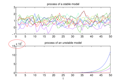
Figure 1 shows an example of stochastic processes generated from a stable recurrent network and an unstable recurrent network respectively. In the upper panel, the recurrent network system parameters satisfy the stability condition (A3a), while those in the lower panel violate (A3a). (In both situations, the number of nodes is 10 and the diffusion parameter $\sigma$ is fixed at $0.5$.) The differences between the two models are obvious.

In reality, asymptotically stable systems are commonly observed. The stability conditions reflect structural characteristics. For example, when all $l_{i}$ are equal and $d_{i}>0$, then the skew-symmetry of ${\boldsymbol{A}}$, i.e., ${\boldsymbol{A}}=-{\boldsymbol{A}}^{\mathsf{T}}$, guarantees asymptotic stability. The information provided by the constrains can assist topology learning. This motivates the design of sparse recurrent network learning with stability.

Figure 1: Stochastic processes generated from a stable recurrent network model and an unstable recurrent network model.

IV-B S³ network estimation

(A3a) is less restrictive than (A3b). In optimization, imposing (A3a) seems however difficult. We propose

$$\begin{gathered}\min_{{\boldsymbol{B}},{\boldsymbol{L}},{\boldsymbol{D}},{\boldsymbol{u}},{\boldsymbol{c}}}\frac{1}{2}\|{\boldsymbol{W}}^{1/2}\{{\boldsymbol{Y}}-[\boldsymbol{\pi}({\boldsymbol{X}}{\boldsymbol{B}}+\boldsymbol{1}{\boldsymbol{u}}^{\mathsf{T}}){\boldsymbol{L}}-{\boldsymbol{X}}{\boldsymbol{D}}+\boldsymbol{1}{\boldsymbol{c}}^{{\mathsf{T}}}]\}\|_{F}^{2}+P({\boldsymbol{B}},{\boldsymbol{\Lambda}})=:F_{1},\\ \mbox{ s.t. }{\boldsymbol{L}}\succeq\boldsymbol{0},{\boldsymbol{D}}\succeq\boldsymbol{0},({\boldsymbol{L}}{\boldsymbol{B}}^{\mathsf{T}}+{\boldsymbol{B}}{\boldsymbol{L}})/2\preceq 4{\boldsymbol{D}},\end{gathered}$$ (25)

referred to as the Stable-Sparse Sigmoidal (S³) network learning. The stability constraints are now imposed on ${\boldsymbol{B}}$ as the transpose of the raw coefficient matrix ${\boldsymbol{A}}$. Similar to the discussion of (19), in implementation, we add mild $\ell_{2}$ penalties on $l_{i}$ and $c_{i}$ to deal with possible collinearity, and it is common to replace $\boldsymbol{0}$ by $\epsilon{\boldsymbol{I}}$ with $\epsilon$ extremely small.

In this part, we focus on the $\ell_{1}$ penalty $P({\boldsymbol{B}},{\boldsymbol{\Lambda}})=\|{\boldsymbol{\Lambda}}\circ{\boldsymbol{B}}\|_{1}$ where matrix $\boldsymbol{\Lambda}$ usually has the form $\boldsymbol{\Lambda}[k,k^{\prime}]=\|{\boldsymbol{X}}[:,k]\|_{2}$ for any $k,k^{\prime}\leq n$ (other options are possible.) Introducing the componentwise regularization matrix is helpful when one wants to maintain or forbid certain links based on prior knowledge or preliminary screening. For example, if no self-regulation is allowed, then all diagonal entries of $\boldsymbol{\Lambda}$ ought to be $+\infty$.

It turns out that one can modify Step 2 and Step 4 of the RNS algorithm to solve (25).

First, the non-negativity of $l_{i}$ and $d_{i}$ can be directly incorporated, if the weighted least-squares problem in Step 2 is replaced by the following programming problem with generalized non-negativity constraints:

Step 2) $$\qquad\mbox{ Solve }\min_{{\boldsymbol{L}},{\boldsymbol{D}},{\boldsymbol{c}}}\|{\boldsymbol{W}}^{1/2}\{{\boldsymbol{Y}}-[{\boldsymbol{\mu}}^{(j)}{\boldsymbol{L}}-{\boldsymbol{X}}{\boldsymbol{D}}+\boldsymbol{1}{\boldsymbol{c}}^{\mathsf{T}}]\}\|_{F}^{2}$$

s.t. $${\boldsymbol{L}}=\mbox{diag}\{l_{i}\}\succeq\boldsymbol{0},{\boldsymbol{D}}=\mbox{diag}\{d_{i}\}\succeq\boldsymbol{0},({\boldsymbol{L}}{\boldsymbol{B}}^{(j-1){\mathsf{T}}}+{\boldsymbol{B}}^{(j-1)}{\boldsymbol{L}})/2\preceq 4{\boldsymbol{D}}.$$ (26)

A variety of algorithms and packages can be used. (The technique in Appendix D also applies.)

Integrating the spectral constraint on ${\boldsymbol{B}}$ into network learning is much trickier. We modify Step 4 of Algorithm 1 as follows.

1. Update ${\boldsymbol{B}}$ and ${\boldsymbol{u}}$:

   1. $\tilde{\boldsymbol{\Xi}}\leftarrow\tilde{\boldsymbol{B}}^{(j-1)}-\tilde{\boldsymbol{X}}^{{\mathsf{T}}}\{\tilde{\boldsymbol{W}}\circ{\boldsymbol{\xi}}(\tilde{\boldsymbol{X}}\tilde{\boldsymbol{B}}^{(j-1)},\tilde{\boldsymbol{Y}})\}({\boldsymbol{K}}^{(j)})^{-}$, ${\boldsymbol{u}}^{(j)}\leftarrow(\tilde{\boldsymbol{\Xi}}[1,:])^{\mathsf{T}}$, ${\boldsymbol{\Xi}}\leftarrow\tilde{\boldsymbol{\Xi}}[2:\mbox{end},:]$, and $\boldsymbol{\Lambda}^{(j)}=\boldsymbol{\Lambda}\cdot({\boldsymbol{K}}^{(j)})^{-}$.

   2. Perform the inner loop iterations, starting with ${\boldsymbol{B}}_{3}\leftarrow\boldsymbol{\Xi}$, ${\boldsymbol{C}}_{3}\leftarrow({\boldsymbol{L}}^{(j)}{\boldsymbol{B}}_{3}^{\mathsf{T}}+{\boldsymbol{B}}_{3}{\boldsymbol{L}}^{(j)})/2$, ${\boldsymbol{P}}=\boldsymbol{0}$, ${\boldsymbol{Q}}_{{\boldsymbol{B}}}=\boldsymbol{0}$, ${\boldsymbol{Q}}_{{\boldsymbol{C}}}=\boldsymbol{0}$, ${\boldsymbol{R}}=\boldsymbol{0}$, and the operators ${\mathcal{P}}^{1},{\mathcal{P}}^{2},{\mathcal{P}}^{3}$ defined in Lemmas 4-6:
      repeat

      1. ${\boldsymbol{B}}_{1}\leftarrow{\mathcal{P}}^{1}({\boldsymbol{B}}_{3}+{\boldsymbol{P}};\boldsymbol{\Lambda}^{(j)})$, ${\boldsymbol{C}}_{1}\leftarrow{\boldsymbol{C}}_{3}$, ${\boldsymbol{P}}\leftarrow{\boldsymbol{P}}+{\boldsymbol{B}}_{3}-{\boldsymbol{B}}_{1}$.

      2. $[{\boldsymbol{B}}_{2},{\boldsymbol{C}}_{2}]\leftarrow{\mathcal{P}}^{2}({\boldsymbol{B}}_{1}+{\boldsymbol{Q}}_{{\boldsymbol{B}}},{\boldsymbol{C}}_{1}+{\boldsymbol{Q}}_{{\boldsymbol{C}}};{\boldsymbol{L}}^{(j)})$,
         ${\boldsymbol{Q}}_{{\boldsymbol{B}}}\leftarrow{\boldsymbol{Q}}_{{\boldsymbol{B}}}+{\boldsymbol{B}}_{1}-{\boldsymbol{B}}_{2}$, ${\boldsymbol{Q}}_{{\boldsymbol{C}}}\leftarrow{\boldsymbol{Q}}_{{\boldsymbol{C}}}+{\boldsymbol{C}}_{1}-{\boldsymbol{C}}_{2}$.

      3. ${\boldsymbol{B}}_{3}\leftarrow{\boldsymbol{B}}_{2}$, ${\boldsymbol{C}}_{3}\leftarrow{\mathcal{P}}^{3}({\boldsymbol{C}}_{2}+{\boldsymbol{R}};{\boldsymbol{D}}^{(j)})$, ${\boldsymbol{R}}\leftarrow{\boldsymbol{R}}+{\boldsymbol{C}}_{2}-{\boldsymbol{C}}_{3}$.

      until convergence
      ${\boldsymbol{B}}^{(j)}\leftarrow{\boldsymbol{B}}_{3}$

   3. $\tilde{\boldsymbol{B}}^{(j)}\leftarrow[{\boldsymbol{u}}^{(j)}\ ({\boldsymbol{B}}^{(j)})^{\mathsf{T}}]^{\mathsf{T}}$

Algorithm 1 with such modifications in Step 2 and Step 4 is referred to as the S³ estimation algorithm.

Theorem 4.

Given any initial point $\tilde{\boldsymbol{B}}^{(0)}$, the S³ algorithm converges in the sense that the function value decreasing property holds, and furthermore, ${\boldsymbol{B}}^{(j)}$, ${\boldsymbol{L}}^{(j)}$, and ${\boldsymbol{D}}^{(j)}$ satisfy ${\boldsymbol{L}}^{(j)}\succeq\boldsymbol{0},{\boldsymbol{D}}^{(j)}\succeq\boldsymbol{0},({\boldsymbol{L}}^{(j)}({\boldsymbol{B}}^{(j)})^{\mathsf{T}}+{\boldsymbol{B}}^{(j)}{\boldsymbol{L}}^{(j)})/2\preceq 4{\boldsymbol{D}}^{(j)}$ for any $j\geq 1$.

The proof is given in Appendix D.

We observe that practically, the inner loop converges fast (usually within 100 steps). Moreover, to guarantee the functional value is decreasing, one does not have to run the inner loop till convergence. Although it is possible to apply the stable-sparse estimation directly, we recommend running the screening algorithm (RNS) first, followed by the fine S³ network learning.

V Experiments

V-A Simulation Studies

In this subsection, we conduct synthetic data experiments to demonstrate the performance of the proposed learning framework in recurrent network analysis. An Erdős-Rényi-like scheme of generating system parameters, including a sparse regulation matrix ${\boldsymbol{A}}$, is described as follows. Given any node $i$, the number of its regulators is drawn from a binomial distribution $\mathcal{B}(n-1,\frac{1}{2n})$. The regulator set $S_{i}$ is chosen randomly from the rest $(n-1)$ nodes (excluding node $i$ itself). If $j\notin S_{i}$, $a_{ij}=0$. Otherwise, $a_{ij}$ follows a mixture of two Gaussians $\mathcal{N}(1.5,0.1^{2})$ ad $\mathcal{N}(-1.5,0.1^{2})$ with probability $1/2$ for each. Then draw random ${\boldsymbol{l}}$, ${\boldsymbol{u}}$, ${\boldsymbol{c}}$ from Gaussian distributions (independently) $l_{i}\sim\mathcal{N}(1.5,0.1^{2}),u_{i}\sim\mathcal{N}(0,0.1^{2}),c_{i}\sim\mathcal{N}(0,0.1^{2})$. Finally $\boldsymbol{d}$ is generated so that the system satisfies the stability condition (A3a).

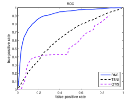
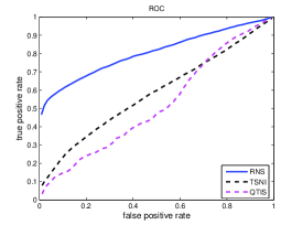
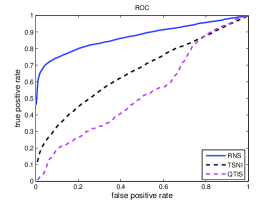
Topology identification. First, we test the performance of RNS in recurrent network topology identification. We compare it with TSNI [25] and QTIS [26]. TSNI is a popular network learning approach and applies principle component analysis for dimensionality reduction. QTIS is a network screening algorithm based on sparsity-inducing techniques. To avoid the ad-hoc issue of parameter tuning, ROC curves will be used to summarize link detection results in a comprehensive way, in terms of true positive rate (TPR) and false positive rate (FPR).

We simulate two networks according to the scheme introduced early. In the first example we set $n=10,T=100$, in the second example $n=200,T=500$, and in the third $n=100,T=1000$. Given all system parameters, we can call Matlab functions sde and sde.simulate to generate continuous-time stochastic processes according to (4). The discrete-time observations are sampled from the stochastic processes with sampling period $\Delta T=1$.

In this experiment, the number of unknowns in either case is larger than the sample size, especially in Ex.2 which has about 41K variables but only 500 observations. Given any algorithm, we vary the target cardinality parameter $m$ from 1 to $n(n-1)$, collect all estimates, and compute their associated TPRs and FPRs. The experiment is repeated for $50$ times and the averaged rates are shown in the ROC curves in Figure 2. RNS beats TSNI and QTIS by a large margin. In fact, the ROC curve of RNS is everywhere above the TSNI curve and the QTIS curve.

(a) Example 1.

(b) Example 2.

(c) Example 3.

Figure 2: Comparison of ROC curves.

System stability. Next, we show the necessity of stable learning in network dynamics forecasting. For simplicity, the $\ell_{1}$ penalization is used. We compare the S³ network estimation with the approach based on sparse sigmoidal regression in Section III-A (with no stability guarantee), denoted by SigSpar.

We use two network examples (Ex.4 and Ex.5) with $n=20,40$ respectively. In each setting, we generate $T=20$ samples for training, and $200$ validation samples for parameter tuning. In this experiment, forecast error at a future time point is the major concern. Suppose ${\boldsymbol{x}}(T)$, the network snapshot at $T$, is given. With system parameter estimates obtained, one can simulate a stochastic process $\boldsymbol{\hat{x}}(t)$ ($t\geq T$) starting with ${\boldsymbol{x}}(T)$ based on model (4). The forecast error at time point $T+h$ is defined as $\mbox{FE}=\|{\boldsymbol{x}}(T+h)-\boldsymbol{\hat{x}}(T+h)\|_{2}^{2}/n$. Long-term forecasting corresponds to large values of $h$. We repeat the experiment for 50 times and show the average FE in Table I. The error of SigSpar becomes extremely large as $h$ increases, because there is no stability guarantee of its network estimate, while S³ has excellent performance even in long-term forecasting.

Table I: Forecasting error comparison on the simulation data.

	$h$	1	5	10	15	20
Ex.4	SigSpar	0.08	3.01	41.95	450.54	4.4$\times$103
	S3	0.04	0.48	1.01	1.39	1.76
Ex.5	SigSpar	0.35	23.76	41.95	7.3$\times$103	1.0$\times$105
	S3	0.06	0.70	1.75	2.80	4.04

V-B Real data

Yeast gene regulatory network. We use RNS to study the transcriptional regulatory network in the yeast cell cycle. The dataset is publicly available and a detailed description of the microarray experiment is in [27]. Following [28], we focus on the 20 genes whose expression patterns fluctuate in a periodic manner. The dataset contains their expression levels recorded at 18 time points during a cell cycle. In this regulatory (sub)network, five genes have been identified as transcription factors, namely SWI4, HCM1, NDD1, SWI5, ASH1, and 19 regulatory connections from them to target genes have been reported with direct evidence in the literature (cf. the YEASTRACT database at http://yeastract.com/). [28] found 55 connections from the transcription factors to the target genes, of which 14 have biological evidence (and so the true positive rate is $14/19=73.7\%$). For a fair comparison, we also let RNS detect 55 connections from the transcription factors to the target genes, and achieved a higher true positive rate $89.5\%$. A detailed comparison of the identified regulatory connections is shown in Table II.

Table II: Regulatory connections of the Yeast cell cycle subnetwork. ‘$\times$’ stands for the regulatory connections identified by RNS, ‘$\underline{\ }$’ stands for those by [28], and ‘$\square$’ stands for the confirmed regulatory connections with published evidence in the literature.

	SWI4	HCM1	NDD1	SWI5	ASH1
SWI4
HCM1	$\underline{\boxtimes}$
NDD1	$\underline{\boxtimes}$
SWI5
ASH1				$\underline{\boxtimes}$
CLN2	$\underline{\boxtimes}$
SVS1	$\underline{\boxtimes}$
SWE1	$\underline{\boxtimes}$
MNN1	$\underline{\boxtimes}$
CLB6	$\underline{\boxtimes}$
HTA1	$\underline{\boxtimes}$
HTB1	$\underline{\boxtimes}$
HHT1
CLB4				$\boxtimes$
CLB2	$\boxtimes$		$\underline{\boxtimes}$
CDC20
SPO12			$\underline{\square}$
SIC1				$\underline{\boxtimes}$
CLN3	$\boxtimes$	$\boxtimes$		$\underline{\boxtimes}$	$\square$
CDC46

fMRI data. The resting state fMRI data provided by the ADHD-200 consortium [29] have been preprocessed by the NIAK interface [30]. The dataset we are using has 954 ROIs (regions of interest) and 257 time points. In the experiment, the first 200 observations are for training (and so $T=200$ and $n=954$), and the following 57 observations are for testing. We applied RNS to get a network pattern, followed by the S³ network estimation for stability correction. Table III shows the results averaged over 10 randomly chosen subjects. Our learning algorithm can achieve much lower error than TSNI, and its performance is pretty robust to the choice of $m$.

Table III: Forecast error on the fMRI data.

$m/n^{2}$	0.5	0.6	0.7	0.8	0.9
TSNI	0.981	1.021	1.044	1.056	1.060
S3	0.194	0.194	0.194	0.194	0.194

Appendix A Proof of Theorem 1

For notation simplicity, we introduce $\mu_{s}({\boldsymbol{\beta}}):=\pi(\tilde{\boldsymbol{x}}_{s}^{{\mathsf{T}}}{\boldsymbol{\beta}})$. Then $\partial\mu_{s}({\boldsymbol{\beta}})/\partial{\boldsymbol{\beta}}=\mu_{s}({\boldsymbol{\beta}})(1-\mu_{s}({\boldsymbol{\beta}}))\tilde{\boldsymbol{x}}_{s}^{{\mathsf{T}}}$, from which it follows that

$$\nabla(\sum_{s=1}^{T}w_{s}(y_{s}-\mu_{s}({\boldsymbol{\beta}}))^{2}/2)=\tilde{\boldsymbol{X}}^{{\mathsf{T}}}{\boldsymbol{W}}{\boldsymbol{\xi}}(\tilde{\boldsymbol{X}}{\boldsymbol{\beta}},{\boldsymbol{y}}),$$

where ${\boldsymbol{W}}=\mbox{diag}\{w_{s}\}_{s=1}^{T}$ and ${\boldsymbol{\xi}}$ is the function defined in (11) applied componentwise. Moreover, we can compute its Hessian (details omitted)

$${\boldsymbol{H}} =D(\nabla(\sum w_{s}(y_{s}-\mu_{s}({\boldsymbol{\beta}}))^{2}/2))$$

$$=\tilde{\boldsymbol{X}}^{{\mathsf{T}}}{\boldsymbol{W}}\mbox{diag}\left\{\mu_{s}(1-\mu_{s})\right.\left.[\mu_{s}(1-\mu_{s})+(\mu_{s}-y_{s})(1-2\mu_{s})]\right\}\tilde{\boldsymbol{X}}$$

$$=:\tilde{\boldsymbol{X}}^{{\mathsf{T}}}{\boldsymbol{W}}{\boldsymbol{\Sigma}}({\boldsymbol{\beta}})\tilde{\boldsymbol{X}}.$$

Note that ${\boldsymbol{H}}$ is not necessarily positive semi-definite.

Let $F_{0}({\boldsymbol{\beta}})=\frac{1}{2}\sum w_{s}(y_{s}-\mu_{s}({\boldsymbol{\beta}}))^{2}+\sum P(\beta_{k};\lambda)$. Define a surrogate function as $G({\boldsymbol{\beta}},{\boldsymbol{\beta}}^{\prime})=\frac{1}{2}\sum w_{s}(y_{s}-\mu_{s}({\boldsymbol{\beta}}^{\prime}))^{2}+\sum P(\beta_{k}^{\prime};\lambda)+\frac{K}{2}\|{\boldsymbol{\beta}}-{\boldsymbol{\beta}}^{\prime}\|_{2}^{2}+\frac{1}{2}\sum w_{s}((y_{s}-\mu_{s}({\boldsymbol{\beta}}))^{2}-(y_{s}-\mu_{s}({\boldsymbol{\beta}}^{\prime}))^{2})+\sum w_{s}\xi({\boldsymbol{x}}_{s}^{{\mathsf{T}}}{\boldsymbol{\beta}},y_{s})({\boldsymbol{x}}_{s}^{{\mathsf{T}}}{\boldsymbol{\beta}}^{\prime}-{\boldsymbol{x}}_{s}^{{\mathsf{T}}}{\boldsymbol{\beta}}).$ Based on the previous calculation, we have

$$\frac{1}{2}\sum w_{s}((y_{s}-\mu_{s}({\boldsymbol{\beta}}))^{2}-(y_{s}-\mu_{s}({\boldsymbol{\beta}}^{\prime}))^{2})$$

$$= (\tilde{\boldsymbol{X}}^{\mathsf{T}}{\boldsymbol{W}}{\boldsymbol{\xi}}(\tilde{\boldsymbol{X}}{\boldsymbol{\beta}},{\boldsymbol{y}}))^{\mathsf{T}}({\boldsymbol{\beta}}-{\boldsymbol{\beta}}^{\prime})-\frac{1}{2}({\boldsymbol{\beta}}-{\boldsymbol{\beta}}^{\prime})^{\mathsf{T}}(\tilde{\boldsymbol{X}}^{\mathsf{T}}{\boldsymbol{W}}{\boldsymbol{\Sigma}}(\theta{\boldsymbol{\beta}}+(1-\theta){\boldsymbol{\beta}}^{\prime})\tilde{\boldsymbol{X}})({\boldsymbol{\beta}}-{\boldsymbol{\beta}}^{\prime}),$$

for some $\theta\in[0,1]$. Let $\boldsymbol{\zeta}=\theta{\boldsymbol{\beta}}+(1-\theta){\boldsymbol{\beta}}^{\prime}$. It follows that

$$\frac{K}{2}\|{\boldsymbol{\beta}}-{\boldsymbol{\beta}}^{\prime}\|_{2}^{2}+\frac{1}{2}\sum w_{s}((y_{s}-\mu_{s}({\boldsymbol{\beta}}))^{2}-(y_{s}-\mu_{s}({\boldsymbol{\beta}}^{\prime}))^{2})$$

$$\quad+\sum w_{s}\xi(\tilde{\boldsymbol{x}}_{s}^{{\mathsf{T}}}{\boldsymbol{\beta}},y_{s})(\tilde{\boldsymbol{x}}_{s}^{{\mathsf{T}}}{\boldsymbol{\beta}}^{\prime}-\tilde{\boldsymbol{x}}_{s}^{{\mathsf{T}}}{\boldsymbol{\beta}})$$

$$= \frac{1}{2}({\boldsymbol{\beta}}^{\prime}-{\boldsymbol{\beta}})^{\mathsf{T}}(K{\boldsymbol{I}}-\tilde{\boldsymbol{X}}^{{\mathsf{T}}}{\boldsymbol{\Sigma}}(\boldsymbol{\zeta}){\boldsymbol{W}}\tilde{\boldsymbol{X}})({\boldsymbol{\beta}}^{\prime}-{\boldsymbol{\beta}})$$

$$\geq \frac{K-\|\tilde{\boldsymbol{X}}\|_{2}^{2}\|{\boldsymbol{\Sigma}}(\boldsymbol{\zeta}){\boldsymbol{W}}\|_{2}}{2}\|{\boldsymbol{\beta}}-{\boldsymbol{\beta}}^{\prime}\|_{2}^{2}.$$

Because

$$w_{s}\mu_{s}(1-\mu_{s})((1-2\mu_{s})(\mu_{s}-y_{s})+\mu_{s}(1-\mu_{s}))$$

$$\leq \frac{w_{s}}{4}\left(\frac{1}{2}\left(\frac{1-2\mu_{s}+2\mu_{s}-2y_{s}}{2}\right)^{2}+\frac{1}{4}\right)$$

$$= \frac{w_{s}}{4}\left(\frac{(1-2y_{s})^{2}}{8}+\frac{1}{4}\right),$$

the diagonal entries of ${\boldsymbol{W}}{\boldsymbol{\Sigma}}(\boldsymbol{\zeta})$ are uniformly bounded by

$$\max_{s}\frac{w_{s}}{4}\left(\frac{(1-2y_{s})^{2}}{8}+\frac{1}{4}\right)$$

or $k_{0}({\boldsymbol{y}},{\boldsymbol{w}})$ (see (12)). Therefore, choosing $K\geq k_{0}({\boldsymbol{y}},{\boldsymbol{w}})\|\tilde{\boldsymbol{X}}\|_{2}^{2}$, we have $G({\boldsymbol{\beta}},{\boldsymbol{\beta}}^{\prime})=\frac{1}{2}\sum w_{s}(y_{s}-\mu_{s}({\boldsymbol{\beta}}^{\prime}))^{2}+\sum P(\beta_{k}^{\prime};\lambda)+\frac{1}{2}(K-\|\tilde{\boldsymbol{X}}\|_{2}^{2}\|{\boldsymbol{W}}{\boldsymbol{\Sigma}}\|_{2}^{2})\geq F_{0}({\boldsymbol{\beta}})$ for any ${\boldsymbol{\beta}},{\boldsymbol{\beta}}^{\prime}$.

On the other hand, based on the definition, it is easy to show (details omitted) that given ${\boldsymbol{\beta}}$, $\min_{{\boldsymbol{\beta}}^{\prime}}G({\boldsymbol{\beta}},{\boldsymbol{\beta}}^{\prime})$ is equivalent to:

$$\min_{{\boldsymbol{\beta}}^{\prime}}\frac{K}{2}\|{\boldsymbol{\beta}}^{\prime}-{\boldsymbol{\beta}}+\frac{1}{K}\tilde{\boldsymbol{X}}^{{\mathsf{T}}}{\boldsymbol{W}}{\boldsymbol{\xi}}(\tilde{\boldsymbol{X}}{\boldsymbol{\beta}},{\boldsymbol{y}})\|_{2}^{2}+\sum P(\beta_{k}^{\prime};\lambda).$$ (27)

Applying Lemma 1 in [16] without requiring uniqueness, there exists a globally optimal solution

$${\boldsymbol{\beta}}_{o}^{\prime}({\boldsymbol{\beta}})=\Theta({\boldsymbol{\beta}}-\tilde{\boldsymbol{X}}^{{\mathsf{T}}}{\boldsymbol{W}}{\boldsymbol{\xi}}(\tilde{\boldsymbol{X}}{\boldsymbol{\beta}},{\boldsymbol{y}})/K;\lambda^{\prime}),$$ (28)

provided that $P(t;\lambda^{\prime})=P(t;\lambda)/K$ for any $t$. In summary, we obtain $F_{0}({\boldsymbol{\beta}})=G({\boldsymbol{\beta}},{\boldsymbol{\beta}})\geq G({\boldsymbol{\beta}},{\boldsymbol{\beta}}_{o}^{\prime}({\boldsymbol{\beta}}))\geq F_{0}({\boldsymbol{\beta}}_{o}^{\prime}({\boldsymbol{\beta}}))$.

We are now in a position to prove (16). In fact, given ${\boldsymbol{\gamma}}$ and $l$, the optimization problem

$$\min_{{\boldsymbol{\beta}}}\frac{1}{2}\sum w_{s}(y_{s}-{\boldsymbol{z}}_{s}^{\mathsf{T}}{\boldsymbol{\gamma}}-l\pi(\tilde{\boldsymbol{x}}_{s}^{{\mathsf{T}}}{\boldsymbol{\beta}}))^{2}+\sum P(\beta_{k},\lambda),$$

is equivalent to $\min_{{\boldsymbol{\beta}}}\frac{1}{2}\sum w_{s}^{\prime}(\tilde{y}_{s}-\pi(\tilde{\boldsymbol{x}}_{s}^{{\mathsf{T}}}{\boldsymbol{\beta}}))^{2}+\sum P(\beta_{k},\lambda)$ with $\tilde{y}_{s}=(y_{s}-{\boldsymbol{z}}_{s}^{\mathsf{T}}{\boldsymbol{\gamma}})/l$, $w_{s}^{\prime}=l^{2}w_{s}$. (Note that the $l$ obtained from WLS is nonzero with probability 1.) Therefore, the function value decreasing property always holds during the iteration.

Appendix B Proof of Theorem 2

Define a quantile thresholding rule $\Theta^{\#}(\cdot;m,\eta)$ as a variant of the hard-ridge thresholding rule (9). Given $1\leq m\leq np$: $\boldsymbol{A}\in\mathcal{R}^{n\times p}\rightarrow{\boldsymbol{B}}\in\mathcal{R}^{n\times p}$ is defined as follows: $b_{ij}=a_{ij}/(1+\eta)$ if $|a_{ij}|$ is among the $m$ largest in the set of $\{|a_{ij}|:1\leq i\leq n,1\leq j\leq p\}$, and $b_{ij}=0$ otherwise.

Lemma 1.

$\boldsymbol{\hat{B}}=\Theta^{\#}(\boldsymbol{A};m,\eta)$ is a globally optimal solution to

$$\begin{gathered}\min_{{\boldsymbol{B}}}f_{0}({\boldsymbol{A}})=\frac{1}{2}\|\boldsymbol{A}-{\boldsymbol{B}}\|_{F}^{2}+\frac{\eta}{2}\|{\boldsymbol{B}}\|_{F}^{2}\\ \mbox{s.t. }\|{\boldsymbol{B}}\|_{0}\leq m.\end{gathered}$$

Proof.

Let $I\subset\{(i,j)|1\leq i\leq n,1\leq j\leq p\}$ with $|I|=m$. Assuming ${\boldsymbol{B}}_{I^{c}}=\boldsymbol{0}$, we get the optimal solution $\boldsymbol{\hat{B}}$ with $\boldsymbol{\hat{B}}=\frac{1}{1+\eta}\boldsymbol{A}_{I}$. It follows that $f_{0}(\boldsymbol{\hat{B}})=\frac{1}{2}\|\boldsymbol{A}\|_{F}^{2}-\frac{1}{2}\sum_{i,j\in I}a_{ij}^{2}$. Therefore, the quantile thresholding $\Theta^{\#}(\boldsymbol{A};m,\eta)$ yields a global minimizer. ∎

Using Lemma 1, we can prove the function value decreasing property; the remaining part follows similar lines of Theorem 1 because of the separability of $F$.

Appendix C Proof of Theorem 3

Let ${\boldsymbol{f}}({\boldsymbol{x}})={\boldsymbol{L}}{\boldsymbol{\pi}}({\boldsymbol{A}}{\boldsymbol{x}}+{\boldsymbol{u}})-{\boldsymbol{D}}{\boldsymbol{x}}+{\boldsymbol{c}}$, where ${\boldsymbol{x}}$ is short for ${\boldsymbol{x}}(t)$. First, we prove the existence of an equilibrium. It suffices to show that there is a solution to ${\boldsymbol{f}}({\boldsymbol{x}})=\boldsymbol{0}$ or ${\boldsymbol{x}}={\boldsymbol{D}}^{-1}{\boldsymbol{L}}{\boldsymbol{\pi}}({\boldsymbol{A}}{\boldsymbol{x}}+{\boldsymbol{u}})+{\boldsymbol{D}}^{-1}{\boldsymbol{c}}=:\varphi({\boldsymbol{x}})$. Obviously, the mapping $\varphi$ is continuous and bounded (say $\|\varphi\|_{\infty}\leq M$), Brouwer’s fixed point theorem [31] indicates the existence of at least one equilibrium in $[-M,M]^{n}$.

Let ${\boldsymbol{x}}^{*}$ be an equilibrium point, i.e., ${\boldsymbol{f}}({\boldsymbol{x}}^{*})=\boldsymbol{0}$. Construct a Lyapunov function candidate $V({\boldsymbol{x}})=\frac{1}{2}({\boldsymbol{x}}-{\boldsymbol{x}}^{*})^{{\mathsf{T}}}{\boldsymbol{P}}({\boldsymbol{x}}-{\boldsymbol{x}}^{*})$ with ${\boldsymbol{P}}$ positive definite and to be determined. Then

$$\frac{\,\mathrm{d}V({\boldsymbol{x}})}{\,\mathrm{d}t}=V^{\prime}({\boldsymbol{x}}){\boldsymbol{f}}({\boldsymbol{x}})$$

$$= ({\boldsymbol{x}}-{\boldsymbol{x}}^{*})^{{\mathsf{T}}}{\boldsymbol{P}}{\boldsymbol{f}}({\boldsymbol{x}})$$

$$= ({\boldsymbol{x}}-{\boldsymbol{x}}^{*})^{{\mathsf{T}}}{\boldsymbol{P}}({\boldsymbol{f}}({\boldsymbol{x}})-{\boldsymbol{f}}({\boldsymbol{x}}^{*}))$$

$$= -({\boldsymbol{x}}-{\boldsymbol{x}}^{*})^{{\mathsf{T}}}{\boldsymbol{P}}{\boldsymbol{D}}({\boldsymbol{x}}-{\boldsymbol{x}}^{*})+({\boldsymbol{x}}-{\boldsymbol{x}}^{*})^{{\mathsf{T}}}{\boldsymbol{P}}{\boldsymbol{L}}({\boldsymbol{\pi}}({\boldsymbol{A}}{\boldsymbol{x}}+{\boldsymbol{u}})-{\boldsymbol{\pi}}({\boldsymbol{A}}{\boldsymbol{x}}^{*}+{\boldsymbol{u}}))$$

$$= -({\boldsymbol{x}}-{\boldsymbol{x}}^{*})^{{\mathsf{T}}}({\boldsymbol{P}}{\boldsymbol{D}}-{\boldsymbol{P}}{\boldsymbol{L}}{\boldsymbol{G}}{\boldsymbol{A}})({\boldsymbol{x}}-{\boldsymbol{x}}^{*})$$

$$= -({\boldsymbol{x}}-{\boldsymbol{x}}^{*})^{{\mathsf{T}}}\left(\frac{{\boldsymbol{P}}{\boldsymbol{D}}+{\boldsymbol{D}}{\boldsymbol{P}}^{{\mathsf{T}}}}{2}-\frac{{\boldsymbol{P}}{\boldsymbol{L}}{\boldsymbol{G}}{\boldsymbol{A}}+{\boldsymbol{A}}^{{\mathsf{T}}}{\boldsymbol{G}}{\boldsymbol{L}}{\boldsymbol{P}}^{{\mathsf{T}}}}{2}\right)({\boldsymbol{x}}-{\boldsymbol{x}}^{*}),$$

where

$${\boldsymbol{G}}=\mbox{diag}\left\{\frac{\pi({\boldsymbol{\alpha}}_{i}^{{\mathsf{T}}}{\boldsymbol{x}}+{\boldsymbol{u}})-\pi({\boldsymbol{\alpha}}_{i}^{{\mathsf{T}}}{\boldsymbol{x}}^{*}+{\boldsymbol{u}})}{{\boldsymbol{\alpha}}_{i}^{{\mathsf{T}}}x_{i}-{\boldsymbol{\alpha}}_{i}^{{\mathsf{T}}}x_{i}^{*}}\right\}.$$

It is easy to verify that ${\boldsymbol{G}}=\mbox{diag}\{{\boldsymbol{\pi}}^{\prime}({\boldsymbol{\xi}})\}\preceq{\boldsymbol{I}}/4$, and thus ${\boldsymbol{P}}{\boldsymbol{L}}{\boldsymbol{G}}{\boldsymbol{A}}+{\boldsymbol{A}}^{{\mathsf{T}}}{\boldsymbol{G}}{\boldsymbol{L}}{\boldsymbol{P}}^{{\mathsf{T}}}\preceq({\boldsymbol{P}}{\boldsymbol{L}}{\boldsymbol{A}}+{\boldsymbol{A}}^{{\mathsf{T}}}{\boldsymbol{L}}{\boldsymbol{P}}^{{\mathsf{T}}})/4$. It is well known [21] that under (A3a), the Lyapunov equation

$${\boldsymbol{P}}\left({\boldsymbol{D}}-\frac{{\boldsymbol{L}}{\boldsymbol{A}}}{4}\right)+\left({\boldsymbol{D}}-\frac{{\boldsymbol{L}}{\boldsymbol{A}}}{4}\right)^{{\mathsf{T}}}{\boldsymbol{P}}^{{\mathsf{T}}}=-{\boldsymbol{R}}$$ (29)

is solvable and uniquely determines a positive definite ${\boldsymbol{P}}$ for any positive definite ${\boldsymbol{R}}$. Therefore, $V$ is indeed a Lyapunov function for the nonlinear dynamical system (22). Moreover, (A3a) implies

$$\frac{\,\mathrm{d}V({\boldsymbol{x}})}{\,\mathrm{d}t}\leq-\varepsilon_{0}\|{\boldsymbol{x}}-{\boldsymbol{x}}^{*}\|_{2}^{2}\leq-\varepsilon V({\boldsymbol{x}})$$

for some $\varepsilon_{0},\varepsilon>0$. By the Lyapunov stability theory—see, e.g., [32] (Chapter 3), (22) must be globally exponentially stable. The uniqueness of the equilibrium is implied by the global exponential stability.

The second result can be shown by setting ${\boldsymbol{P}}={\boldsymbol{I}}$ in (29); details are omitted.

Appendix D Proof of Theorem 4

Based on the proof of Theorem 1, the modified Step 2 does not affect the convergence of function value because at each iteration a global optimum of (26) is obtained. It remains to show that $\tilde{\boldsymbol{B}}^{(j)}$ generated by the modified Step 4 improves $\tilde{\boldsymbol{B}}^{(j-1)}$ in terms of reducing the objective function value, and ${\boldsymbol{B}}^{(j)}$ obeys the stability condition.

Let $\tilde{\boldsymbol{\Xi}}=\tilde{\boldsymbol{B}}^{(j-1)}-\tilde{\boldsymbol{X}}^{{\mathsf{T}}}{\boldsymbol{W}}{\boldsymbol{\xi}}(\tilde{\boldsymbol{X}}\tilde{\boldsymbol{B}}^{(j-1)},\tilde{\boldsymbol{Y}})({\boldsymbol{K}}^{(j)})^{-}$, $\boldsymbol{\Lambda}^{(j)}=\boldsymbol{\Lambda}\cdot({\boldsymbol{K}}^{(j)})^{-}$. (The modified Step 2 may result in zeros in $\tilde{\boldsymbol{\Xi}}$ to make the associated activation terms in $\boldsymbol{\pi}(\tilde{\boldsymbol{X}}\tilde{\boldsymbol{B}})$ vanish; using the pseudoinverse can handle the issue and maintain the decreasing property.) Based on the argument of Appendix A, the problem in Step 4 reduces to

$$\begin{split}\min_{\tilde{\boldsymbol{B}}=[{\boldsymbol{u}},{\boldsymbol{B}}^{\mathsf{T}}]^{\mathsf{T}}}\frac{1}{2}\|\tilde{\boldsymbol{B}}-\tilde{\boldsymbol{\Xi}}\|_{F}^{2}+\|\boldsymbol{\Lambda}^{(j)}\circ{\boldsymbol{B}}\|_{1},\\ \mbox{ s.t. }({\boldsymbol{L}}^{(j)}{\boldsymbol{B}}^{\mathsf{T}}+{\boldsymbol{B}}{\boldsymbol{L}}^{(j)})/2\preceq 4{\boldsymbol{D}}^{(j)}.\end{split}$$ (30)

Therefore it suffices to prove Lemma 2 for any given ${\boldsymbol{\Xi}}(=\tilde{\boldsymbol{\Xi}}[2:\mbox{end},:])$, $\boldsymbol{\Lambda}^{(j)}$, ${\boldsymbol{L}}^{(j)}\succeq\boldsymbol{0}$, ${\boldsymbol{D}}^{(j)}\succeq\boldsymbol{0}$, and ${\boldsymbol{B}}^{(j-1)}$. (In fact, the lemma holds given any initialization of ${\boldsymbol{C}}_{3}$.)

Lemma 2.

For any $j\geq 1$, , $\frac{1}{2}\|{\boldsymbol{B}}^{(j)}-{\boldsymbol{\Xi}}\|_{F}^{2}+\|\boldsymbol{\Lambda}^{(j)}\circ{\boldsymbol{B}}^{(j)}\|_{1}\leq\frac{1}{2}\|{\boldsymbol{B}}^{(j-1)}-{\boldsymbol{\Xi}}\|_{F}^{2}+\|\boldsymbol{\Lambda}^{(j)}\circ{\boldsymbol{B}}^{(j-1)}\|_{1}$, and $({\boldsymbol{L}}^{(j)}{\boldsymbol{B}}^{(j){\mathsf{T}}}+{\boldsymbol{B}}^{(j)}{\boldsymbol{L}}^{(j)})/2\preceq 4{\boldsymbol{D}}^{(j)}$.

Proof.

Define $f({\boldsymbol{B}})=\frac{1}{2}\|{\boldsymbol{B}}-{\boldsymbol{\Xi}}\|_{F}^{2}+\|\boldsymbol{\Lambda}\circ{\boldsymbol{B}}\|_{1}$, and $g({\boldsymbol{B}}^{\prime},{\boldsymbol{C}}^{\prime},{\boldsymbol{B}},{\boldsymbol{C}})=\frac{1}{2}\|{\boldsymbol{B}}^{\prime}-{\boldsymbol{\Xi}}\|_{F}^{2}+\|\boldsymbol{\Lambda}\circ{\boldsymbol{B}}\|_{1}+\frac{1}{2}\|{\boldsymbol{B}}-{\boldsymbol{B}}^{\prime}\|_{F}^{2}+\frac{1}{2}\|{\boldsymbol{C}}-{\boldsymbol{C}}^{\prime}\|_{F}^{2}+\langle{\boldsymbol{B}}^{\prime}-{\boldsymbol{\Xi}},{\boldsymbol{B}}-{\boldsymbol{B}}^{\prime}\rangle$. Then $f({\boldsymbol{B}}^{\prime})=g({\boldsymbol{B}}^{\prime},{\boldsymbol{C}}^{\prime},{\boldsymbol{B}}^{\prime},{\boldsymbol{C}}^{\prime})$ and $g({\boldsymbol{B}}^{\prime},{\boldsymbol{C}}^{\prime},{\boldsymbol{B}},{\boldsymbol{C}})\geq f({\boldsymbol{B}})$.

On the other hand, given $({\boldsymbol{B}}^{\prime},{\boldsymbol{C}}^{\prime})$, we can write $g$ as a function of $({\boldsymbol{B}},{\boldsymbol{C}})$: $\frac{1}{2}\|[\boldsymbol{\Xi},\boldsymbol{C}^{\prime}]-[{\boldsymbol{B}},{\boldsymbol{C}}]\|_{F}^{2}+\|\boldsymbol{\Lambda}\circ{\boldsymbol{B}}\|_{1}$ (up to additive functions of ${\boldsymbol{B}}^{\prime}$ and ${\boldsymbol{C}}^{\prime}$). Based on Lemma 3, with $\boldsymbol{\Xi}_{{\boldsymbol{C}}}={\boldsymbol{C}}^{\prime}$, $g({\boldsymbol{B}}^{\prime},{\boldsymbol{C}}^{\prime},{\boldsymbol{B}}^{\prime},{\boldsymbol{C}}^{\prime})\geq g({\boldsymbol{B}}^{\prime},{\boldsymbol{C}}^{\prime},{\boldsymbol{B}}^{o},{\boldsymbol{C}}^{o})\geq f({\boldsymbol{B}}^{o})$ and $({\boldsymbol{L}}{{\boldsymbol{B}}^{o}}^{\mathsf{T}}+{\boldsymbol{B}}^{o}{\boldsymbol{L}})/2={\boldsymbol{C}}^{o}\preceq 4{\boldsymbol{D}}$.

Applying the result to the modified Step 4 in Section IV-B yields the desired result. ∎

Lemma 3.

Consider the sequence of $({\boldsymbol{B}}_{3},{\boldsymbol{C}}_{3})$ generated by the following procedure, with the operators $\mathcal{P}^{1}$, $\mathcal{P}^{2}$, $\mathcal{P}^{3}$ defined in Lemma 4, Lemma 5 and Lemma 6, respectively:

  0) ${\boldsymbol{B}}_{3}\leftarrow\boldsymbol{\Xi}_{{\boldsymbol{B}}}$, ${\boldsymbol{C}}_{3}\leftarrow\boldsymbol{\Xi}_{{\boldsymbol{C}}}$, ${\boldsymbol{P}}=\boldsymbol{0}$, ${\boldsymbol{Q}}_{{\boldsymbol{B}}}=\boldsymbol{0}$, ${\boldsymbol{Q}}_{{\boldsymbol{C}}}=\boldsymbol{0}$, ${\boldsymbol{R}}=\boldsymbol{0}$

  repeat

     1) ${\boldsymbol{B}}_{1}\leftarrow{\mathcal{P}}^{1}({\boldsymbol{B}}_{3}+{\boldsymbol{P}};\boldsymbol{\Lambda})$, ${\boldsymbol{C}}_{1}\leftarrow{\boldsymbol{C}}_{3}$, ${\boldsymbol{P}}\leftarrow{\boldsymbol{P}}+{\boldsymbol{B}}_{3}-{\boldsymbol{B}}_{1}$

     2) $[{\boldsymbol{B}}_{2},{\boldsymbol{C}}_{2}]\leftarrow{\mathcal{P}}^{2}({\boldsymbol{B}}_{1}+{\boldsymbol{Q}}_{{\boldsymbol{B}}},{\boldsymbol{C}}_{1}+{\boldsymbol{Q}}_{{\boldsymbol{C}}};{\boldsymbol{L}})$, $[{\boldsymbol{Q}}_{{\boldsymbol{B}}},{\boldsymbol{Q}}_{{\boldsymbol{C}}}]\leftarrow[{\boldsymbol{Q}}_{{\boldsymbol{B}}},{\boldsymbol{Q}}_{{\boldsymbol{C}}}]+[{\boldsymbol{B}}_{1},{\boldsymbol{C}}_{1}]-[{\boldsymbol{B}}_{2},{\boldsymbol{C}}_{2}]$

     3) ${\boldsymbol{B}}_{3}\leftarrow{\boldsymbol{B}}_{2}$, ${\boldsymbol{C}}_{3}\leftarrow{\mathcal{P}}^{3}({\boldsymbol{C}}_{2}+{\boldsymbol{R}};{\boldsymbol{D}})$, ${\boldsymbol{R}}\leftarrow{\boldsymbol{R}}+{\boldsymbol{C}}_{2}-{\boldsymbol{C}}_{3}$.

  until convergence

Then, the sequence of iterates converges to a globally optimal solution $({\boldsymbol{B}}^{o},{\boldsymbol{C}}^{o})$ to

$$\begin{split}\min_{{\boldsymbol{B}},{\boldsymbol{C}}}\frac{1}{2}\|[\boldsymbol{\Xi}_{{\boldsymbol{B}}},\boldsymbol{\Xi}_{{\boldsymbol{C}}}]-[{\boldsymbol{B}},{\boldsymbol{C}}]\|_{F}^{2}+\|\boldsymbol{\Lambda}\circ{\boldsymbol{B}}\|_{1}\\ \mbox{ s.t. }{\boldsymbol{C}}=({\boldsymbol{L}}{\boldsymbol{B}}^{\mathsf{T}}+{\boldsymbol{B}}{\boldsymbol{L}})/2,{\boldsymbol{C}}\preceq 4{\boldsymbol{D}}.\end{split}$$ (31)

Proof.

With the following three lemmas, applying Theorem 3.2 and Theorem 3.3 in [33] yields the strict convergence of the iterates and the global optimality of the limit point. ∎

Lemma 4.

Let $\mathcal{P}^{1}(\boldsymbol{\Phi})$ be the optimal solution to

$$\min_{{\boldsymbol{B}}}\frac{1}{2}\|{\boldsymbol{B}}-\boldsymbol{\Phi}\|_{F}^{2}+\|\boldsymbol{\Lambda}\circ{\boldsymbol{B}}\|_{1}.$$ (32)

Then $\mathcal{P}^{1}(\boldsymbol{\Phi};\boldsymbol{\Lambda})=\Theta_{S}(\boldsymbol{\Phi};\boldsymbol{\Lambda})$ where $\Theta_{S}$, applied componentwise on $\boldsymbol{\Phi}$, is the soft-thresholding rule given in Section III-A.

Proof.

Apply Lemma 1 in [16]. ∎

Lemma 5.

The optimal solution to

$$\min_{{\boldsymbol{B}},{\boldsymbol{C}}}\frac{1}{2}\|[{\boldsymbol{B}}\ {\boldsymbol{C}}]-[\boldsymbol{\Phi}_{{\boldsymbol{B}}}\ \boldsymbol{\Phi}_{{\boldsymbol{C}}}]\|_{F}^{2}\mbox{ s.t. }{\boldsymbol{C}}=({\boldsymbol{L}}{\boldsymbol{B}}^{\mathsf{T}}+{\boldsymbol{B}}{\boldsymbol{L}})/2.$$ (33)

is given by $\mathcal{P}^{2}(\boldsymbol{\Phi}_{{\boldsymbol{B}}},\boldsymbol{\Phi}_{{\boldsymbol{C}}};{\boldsymbol{L}})=[{\boldsymbol{B}}^{o},{\boldsymbol{C}}^{o}]$ with ${\boldsymbol{B}}^{o}=[b_{i,j}^{o}]$, $b_{i,j}^{o}=\psi_{i,j}\frac{2+l_{i}^{2}}{2+l_{i}^{2}+l_{j}^{2}}-\psi_{j,i}\frac{l_{i}l_{j}}{2+l_{i}^{2}+l_{j}^{2}}$, and ${\boldsymbol{C}}^{o}=({\boldsymbol{L}}{{\boldsymbol{B}}^{o}}^{{\mathsf{T}}}+{{\boldsymbol{B}}^{o}}^{{\mathsf{T}}}{\boldsymbol{L}})/2$, where $\boldsymbol{\Psi}=[\psi_{i,j}]=\boldsymbol{\Phi}_{{\boldsymbol{B}}}+(\boldsymbol{\Phi}_{{\boldsymbol{C}}}+\boldsymbol{\Phi}_{{\boldsymbol{C}}}^{\mathsf{T}}){\boldsymbol{L}}/2$.

Proof.

Let $f({\boldsymbol{B}})=\|{\boldsymbol{B}}-\boldsymbol{\Phi}_{{\boldsymbol{B}}}\|_{F}^{2}/2+\|({\boldsymbol{L}}{\boldsymbol{B}}^{\mathsf{T}}+{\boldsymbol{B}}{\boldsymbol{L}})/2-\boldsymbol{\Phi}_{{\boldsymbol{C}}}\|_{F}^{2}/2$. It is not difficult to obtain the gradient (details omitted): ${\boldsymbol{B}}-\boldsymbol{\Phi}_{{\boldsymbol{B}}}+({\boldsymbol{L}}{\boldsymbol{B}}^{\mathsf{T}}{\boldsymbol{L}}+{\boldsymbol{B}}{\boldsymbol{L}}^{2})/2-(\boldsymbol{\Phi}_{{\boldsymbol{C}}}+\boldsymbol{\Phi}_{{\boldsymbol{C}}}^{\mathsf{T}}){\boldsymbol{L}}/2$. The optimal ${\boldsymbol{B}}$ and ${\boldsymbol{C}}$ can be evaluated accordingly. ∎

Lemma 6.

Let $\mathcal{P}^{3}(\boldsymbol{\Phi};{\boldsymbol{D}})$ be the optimal solution to

$$\min_{{\boldsymbol{C}}}\frac{1}{2}\|{\boldsymbol{C}}-\boldsymbol{\Phi}\|_{F}^{2}\mbox{ s.t. }{\boldsymbol{C}}\mbox{ is symmetric and satisfies }{\boldsymbol{C}}\preceq 4\boldsymbol{D}.$$ (34)

Then it is given by $\boldsymbol{U}\mbox{diag}\{\min(s_{i},0)\}\boldsymbol{U}^{{\mathsf{T}}}+4\boldsymbol{D}$, where $\boldsymbol{S}=\mbox{diag}\{s_{1},\cdots,s_{n}\}$ and ${\boldsymbol{U}}$ are from the spectral decomposition of $(\boldsymbol{\Phi}+\boldsymbol{\Phi}^{\mathsf{T}})/{2}-4\boldsymbol{D}=\boldsymbol{U}\boldsymbol{S}\boldsymbol{U}^{{\mathsf{T}}}$.

Proof.

Because ${\boldsymbol{C}}$ is symmetric (but $\boldsymbol{\Phi}$ may not be), we have

$$\|{\boldsymbol{C}}-\boldsymbol{\Phi}\|_{F}^{2}$$ (35)

$$= \sum_{1\leq i<j\leq p}[(c_{ij}-\phi_{ij})^{2}+(c_{ij}-\phi_{ji})^{2}]+\sum_{i=1}^{p}(c_{ii}-\phi_{ii})^{2}$$

$$= \sum_{1\leq i<j\leq p}2(c_{ij}-\frac{\phi_{ij}+\phi_{ji}}{2})^{2}+\sum_{i=1}^{p}(c_{ii}-\phi_{ii})^{2}+const(\boldsymbol{\Phi})$$

$$= \,\|{\boldsymbol{C}}-\frac{\boldsymbol{\Phi}+\boldsymbol{\Phi}^{\mathsf{T}}}{2}\|_{F}^{2}+const(\boldsymbol{\Phi}),$$

where $const(\boldsymbol{\Phi})$ is a term that does not depend on ${\boldsymbol{C}}$. Therefore, problem (34) is equivalent to

$$\begin{gathered}\min_{{\boldsymbol{C}}}\frac{1}{2}\|{\boldsymbol{C}}-\frac{\boldsymbol{\Phi}+\boldsymbol{\Phi}^{\mathsf{T}}}{2}\|_{F}^{2},\mbox{s.t. }{\boldsymbol{C}}-4\boldsymbol{D}\preceq\boldsymbol{0}.\end{gathered}$$ (36)

The optimality of $\mathcal{P}^{3}(\boldsymbol{\Phi};{\boldsymbol{D}})$ can then be argued by von Neumann’s trace inequality [34, 35]. ∎

References

- Faith et al. [2007] J. J. Faith, B. Hayete, J. T. Thaden, I. Mogno, J. Wierzbowski, G. Cottarel, S. Kasif, J. J. Collins, and T. S. Gardner, “Large-scale mapping and validation of escherichia coli transcriptional regulation from a compendium of expression profiles,” PLoS Biol, vol. 5, no. 1, p. e8, Jan. 2007.
- Mills and Markellos [2008] T. Mills and R. Markellos, The econometric modelling of financial time series. Cambridge University Press, 2008.
- Bullmore and Sporns [2009] E. Bullmore and O. Sporns, “Complex brain networks: graph theoretical analysis of structural and functional systems,” Nature Reviews Neuroscience, vol. 10, pp. 186–198, Mar. 2009.
- Hanneke et al. [2010] S. Hanneke, W. Fu, and E. P. Xing, “Discrete temporal models of social networks,” Electronic Journal of Statistics, vol. 4, pp. 585–605, 2010.
- Roebroeck et al. [2005] A. Roebroeck, E. Formisano, and R. Goebel, “Mapping directed influence over the brain using granger causality and fmri,” Neuroimage, vol. 25, no. 1, pp. 230–242, 2005.
- Beer [1997] R. D. Beer, “The dynamics of adaptive behavior: A research program,” Robotics and Autonomous Systems, vol. 20, no. 2, pp. 257–289, 1997.
- Gallacher and Fiore [2000] J. C. Gallacher and J. M. Fiore, “Continuous time recurrent neural networks: a paradigm for evolvable analog controller circuits,” in National Aerospace and Electronics Conference 2000, Proceedings of the IEEE 2000. IEEE, 2000, pp. 299–304.
- Mayer et al. [2006] H. Mayer, F. Gomez, D. Wierstra, I. Nagy, A. Knoll, and J. Schmidhuber, “A system for robotic heart surgery that learns to tie knots using recurrent neural networks,” in Intelligent Robots and Systems, 2006 IEEE/RSJ International Conference on, 2006, pp. 543–548.
- Xu et al. [2007] R. Xu, D. Wunsch II, and R. Frank, “Inference of genetic regulatory networks with recurrent neural network models using particle swarm optimization,” IEEE/ACM Transactions on Computational Biology and Bioinformatics (TCBB), vol. 4, no. 4, pp. 681–692, 2007.
- Vu and Vohradsky [2007] T. T. Vu and J. Vohradsky, “Nonlinear differential equation model for quantification of transcriptional regulation applied to microarray data of saccharomyces cerevisiae,” Nucleic acids research, vol. 35, no. 1, pp. 279–287, 2007.
- Kou et al. [2012] S. C. Kou, B. P. Olding, M. Lysy, and J. S. Liu, “A multiresolution method for parameter estimation of diffusion processes,” Journal of the American Statistical Association, vol. 107, no. 500, pp. 1558–1574, 2012.
- Fujita et al. [2007] A. Fujita, J. Sato, H. Garay-Malpartida, R. Yamaguchi, S. Miyano, M. Sogayar, and C. Ferreira, “Modeling gene expression regulatory networks with the sparse vector autoregressive model,” BMC Systems Biology, vol. 1, no. 1, 2007.
- Granger [1969] C. W. J. Granger, “Investigating causal relations by econometric models and cross-spectral methods,” Econometrica, vol. 37, no. 3, pp. 424–438, 1969.
- Bally and Talay [1996] V. Bally and D. Talay, “The law of the Euler scheme for stochastic differential equations,” Probability theory and related fields, vol. 104, no. 1, pp. 43–60, 1996.
- James and Stein [1961] W. James and C. Stein, “Estimation with quadratic loss,” in Proceedings of the fourth Berkeley symposium on mathematical statistics and probability, vol. 1, no. 1961, 1961, pp. 361–379.
- She [2012] Y. She, “An iterative algorithm for fitting nonconvex penalized generalized linear models with grouped predictors,” Computational Statistics and Data Analysis, vol. 9, pp. 2976–2990, 2012.
- Zou and Hastie [2005] H. Zou and T. Hastie, “Regularization and variable selection via the elastic net,” Journal of the Royal Statistical Society: Series B (Statistical Methodology), vol. 67, no. 2, pp. 301–320, 2005.
- Park and Hastie [2007] M. Y. Park and T. Hastie, “L1-regularization path algorithm for generalized linear models,” Journal of the Royal Statistical Society: Series B (Statistical Methodology), vol. 69, no. 4, pp. 659–677, 2007.
- She and Owen [2011] Y. She and A. Owen, “Outlier detection using nonconvex penalized regression,” Journal of the American Statistical Association, vol. 106, no. 494, pp. 626–639, 2011.
- Sastry [1999] S. Sastry, Nonlinear systems: analysis, stability, and control. Springer New York, 1999, vol. 10.
- LaSalle and Artstein [1976] J. P. LaSalle and Z. Artstein, The stability of dynamical systems. SIAM, 1976, vol. 25.
- Lyapunov [1892] A. Lyapunov, The General Problem of the Stability Of Motion. Kharkov Mathematical Society, 1892.
- Lyapunov [1992] ——, The General Problem of the Stability Of Motion, ser. Control Theory and Applications Series. Taylor & Francis, 1992.
- Cohen and Grossberg [1983] M. A. Cohen and S. Grossberg, “Absolute stability of global pattern formation and parallel memory storage by competitive neural networks,” Systems, Man and Cybernetics, IEEE Transactions on, vol. SMC-13, no. 5, pp. 815–826, 1983.
- Bansal et al. [2006] M. Bansal, G. Della Gatta, and D. Di Bernardo, “Inference of gene regulatory networks and compound mode of action from time course gene expression profiles,” Bioinformatics, vol. 22, no. 7, pp. 815–822, 2006.
- He et al. [2013] Y. He, Y. She, and D. Wu, “Stationary-sparse causality network learning,” Journal of Machine Learning Research, vol. 14, pp. 3073–3104, 2013.
- Spellman et al. [1998] P. T. Spellman, G. Sherlock, M. Q. Zhang, V. R. Iyer, K. Anders, M. B. Eisen, P. O. Brown, D. Botstein, and B. Futcher, “Comprehensive identification of cell cycle–regulated genes of the yeast saccharomyces cerevisiae by microarray hybridization,” Molecular biology of the cell, vol. 9, no. 12, pp. 3273–3297, 1998.
- Chen et al. [2004] H.-C. Chen, H.-C. Lee, T.-Y. Lin, W.-H. Li, and B.-S. Chen, “Quantitative characterization of the transcriptional regulatory network in the yeast cell cycle,” Bioinformatics, vol. 20, no. 12, pp. 1914–1927, 2004.
- Milham et al. [2012] M. P. Milham, D. Fair, M. Mennes, and S. H. Mostofsky, “The adhd-200 consortium: a model to advance the translational potential of neuroimaging in clinical neuroscience,” Frontiers in Systems Neuroscience, vol. 6, p. 62, 2012.
- Lavoie-Courchesne et al. [2012] S. Lavoie-Courchesne, P. Rioux, F. Chouinard-Decorte, T. Sherif, M.-E. Rousseau, S. Das, R. Adalat, J. Doyon, C. Craddock, D. Margulies et al., “Integration of a neuroimaging processing pipeline into a pan-canadian computing grid,” in Journal of Physics: Conference Series, vol. 341, no. 1. IOP Publishing, 2012, p. 012032.
- Brouwer [1911] L. E. J. Brouwer, “Über abbildung von mannigfaltigkeiten,” Mathematische Annalen, vol. 71, no. 1, pp. 97–115, 1911.
- Haddad and Chellaboina [2008] W. M. Haddad and V. Chellaboina, Nonlinear dynamical systems and control: a Lyapunov-based approach. Princeton University Press, 2008.
- Bauschke and Combettes [2008] H. H. Bauschke and P. L. Combettes, “A Dykstra-like algorithm for two monotone operators,” Pacific Journal of Optimization, vol. 4, no. 3, pp. 383–391, Sep. 2008.
- von Neumann [1937] J. von Neumann, “Some matrix inequalities and metrization of matrix space,” Tomsk. Univ. Rev., vol. 1, pp. 153–167, 1937.
- She [2013] Y. She, “Reduced rank vector generalized linear models for feature extraction,” Statistics and Its Interface, vol. 6, pp. 197–209, 2013.