Robust Orthogonal Complement Principal Component Analysis

Abstract

Recently, the robustification of principal component analysis has attracted lots of attention from statisticians, engineers and computer scientists. In this work we study the type of outliers that are not necessarily apparent in the original observation space but can seriously affect the principal subspace estimation. Based on a mathematical formulation of such transformed outliers, a novel robust orthogonal complement principal component analysis (ROC-PCA) is proposed. The framework combines the popular sparsity-enforcing and low rank regularization techniques to deal with row-wise outliers as well as element-wise outliers. A non-asymptotic oracle inequality guarantees the accuracy and high breakdown performance of ROC-PCA in finite samples. To tackle the computational challenges, an efficient algorithm is developed on the basis of Stiefel manifold optimization and iterative thresholding. Furthermore, a batch variant is proposed to significantly reduce the cost in ultra high dimensions. The paper also points out a pitfall of a common practice of SVD reduction in robust PCA. Experiments show the effectiveness and efficiency of ROC-PCA in both synthetic and real data.

Keywords: outliers, manifold optimization, oracle inequalities, low rank approximation, sparsity

1 Introduction

During the past few years, big data arising in machine learning, signal processing, genetics, and many other fields pose a dimensionality challenge in statistical computation and analysis. To uncover low-dimensional structures underlying such high-dimensional data, the principal component analysis (PCA) is one of the most popularly used multivariate dimension reduction tools. Let ${\boldsymbol{X}}\in\mathbb{R}^{n\times p}$ be a data matrix with $n$ observations in $p$-dimensional space. PCA can be characterized by finding a low rank data approximation, i.e., $\min_{{\boldsymbol{B}}}$ $\|\boldsymbol{X-B}\|_{F}^{2}$ subject to $\text{rank}({\boldsymbol{B}})\leq r$. The solution is given by a truncated singular value decomposition (SVD) of ${\boldsymbol{X}}$: $\hat{{\boldsymbol{B}}}={\boldsymbol{U}}\mbox{diag}\{\sigma_{1},...,\sigma_{r}\}{\boldsymbol{V}}^{T}=\boldsymbol{XVV}^{T}$, where ${\boldsymbol{V}}$ consists of the first $r$ right singular vectors of ${\boldsymbol{X}}$ with $\boldsymbol{VV}^{T}$ defining the rank-$r$ principal subspace. The squared error loss function is reasonable under a Gaussian noise model ${\boldsymbol{X}}={\boldsymbol{B}}+{\boldsymbol{E}}$, but is notoriously known to be non-robust and sensitive to atypical observations or the so-called outliers. Outliers typically refer to extreme observations far away from the majority of the data, and occur ubiquitously in real life data (Maronna et al., (2006), Hampel et al., (2011)). They may seriously affect statistical estimation and inference—in fact, a single outlier can break down the PCA completely and result in a misleading subspace estimate.

The robustification of PCA has been extensively studied in robust statistics, e.g., Rousseeuw and Van Driessen, (1999), Locantore et al., (1999), Hubert et al., (2005), among many others. The recent renowned Principal Component Pursuit (PCP) due to Candès et al., (2011) has drawn a lot of attention from researchers even beyond the statistics community. PCP decomposes ${\boldsymbol{X}}$ into a low-rank component ${\boldsymbol{B}}$ and a sparse gross outlier component $\boldsymbol{S}$. The recovery problem can be formulated by $\min_{{\boldsymbol{B}},\boldsymbol{S}}\text{rank}({\boldsymbol{B}})+\lambda\|\boldsymbol{S}\|_{0}$ subject to $\boldsymbol{X}={\boldsymbol{B}}+\boldsymbol{S}$, where $\|\cdot\|_{0}$ denotes the element-wise $\ell_{0}$ norm, i.e., the number of all non-zeros. PCP applies a convex relaxation to facilitate computation and analysis: $\min_{\text{${\boldsymbol{B}}$, $\boldsymbol{S}$}}\|{\boldsymbol{B}}\|_{*}+\lambda\|\boldsymbol{S}\|_{1}\ \ \text{subject to}\ \ \boldsymbol{X}={\boldsymbol{B}}+\boldsymbol{S},$ where $\|\cdot\|_{*}$ denotes the matrix nuclear norm (sum of all singular values), and $\|\cdot\|_{1}$ denotes the element-wise $\ell_{1}$ norm. PCP has various extensions and variants (Zhou et al., (2010), Xu et al., (2010), Wright et al., (2013)), and has widespread applications in image and video analysis, e.g., Wright et al., (2009), Peng et al., (2012), Zhang et al., (2012). Although PCP can effectively deal with additive outliers in the original observation space, it may fail in the presence of another important type of outliers, the so-called OC outliers, which is the major concern of this work.

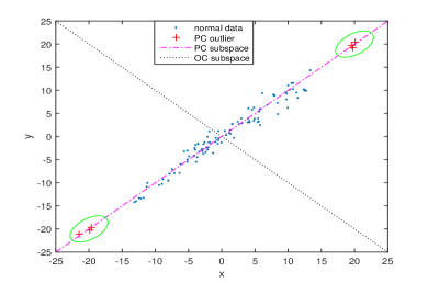
(a) Normal data (’.’) and PC outliers (’+’).

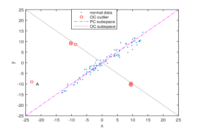
(b) Normal data (’.’) and OC outliers (’o’).

Figure 1: PC outliers and OC outliers.

In robust principal component analysis, the outliers worthy of attention must affect the principal subspace estimation. Figure 1 gives some toy examples to illustrate how outliers could interfere with principal subspace identification. In the left panel, some outlying samples exist in the principal component subspace (PC subspace), which we call pure PC outliers, or PC outliers, for short. Interestingly, they do not affect the detection of PC subspace. PC outliers are not that harmful (though possibly affecting the order of PC directions), and thus, can be handled in a later stage. However, if one only checks the raw $(x$, $y)$ coordinates in the observed space, these samples might be labeled as outliers.

The right panel contains some samples atypical in the orthogonal complement subspace (OC subspace), which we call OC outliers. We emphasize that any points showing outlyingness in OC coordinates are referred to as OC outliers in this paper, such as Point $A$ in Figure 1(b), whether or not they show PC outlyingness. It is the OC outliers that can skew the PC subspace. Unfortunately, checking their coordinates in the observation space offers little help, thereby making PCP possibly fail in recovering the genuine PC subspace. However, if one could project the data points onto the ideal OC subspace, such outliers would be easily revealed and detected.

This paper proposes a novel robust orthogonal complement principal component analysis (ROC-PCA) to address such OC outliers in principal subspace recovery. In contrast to the existing robust PCA approaches, ROC-PCA explicitly deals with OC outliers, and aims at simultaneous outlier identification and robust principal subspace recovery. Both row-wise (r-Type) outliers and element-wise (e-Type) outliers are discussed. Our computation algorithm involves Stiefel manifold optimization and allows for all popular sparsity-enforcing penalties to be used. We also establish a non-asymptotic oracle inequality to provide a theoretical guarantee of ROC-PCA from the predictive learning perspective.

The rest of the paper is organized as follows. Section 2 briefly reviews the existing robust PCA methods and models. Section 3 proposes the ROC-PCA and formulates a useful framework to generalize the $M$-estimators to robust subspace estimation. In Section 4, a class of computational algorithms involving Stiefel manifold optimization and iterative thresholding is proposed. Section 5 theoretically analyzes the performance of ROC-PCA in finite samples. In Section 6, we point out a pitfall of applying a popular SVD reduction in high dimensional robust PCA and propose a batch variant of ROC-PCA for big data computation. Section 7 and Section 8 present extensive numerical studies using both synthetic data and real data, and compare ROC-PCA with some other popular robust PCA approaches. We conclude in Section 9. All technical details are left to the Appendices.

2 Survey of Robust PCA

The non-robustness issue of PCA has been noticed long before and extensively investigated in robust statistics. See, e.g., Maronna et al., (2006) for a comprehensive introduction. In this work, we classify robust PCA approaches into five classes: 1) robust covariance matrix based methods; 2) projection based methods; 3) hybrid projection-covariance estimation based methods; 4) spherical/elliptical PCA; 5) low rank matrix approximation based methods. Due to space limitations, we only review some representative works in each class, which gives by no means a complete list of literature on robust PCA.

Robust covariance matrix based methods

Robust PCA can be achieved by first finding a robust covariance estimate, and then extracting PC loadings from the eigen-decomposition of this matrix. One of the earliest works is Maronna, (1976) that considers multivariate $M$-estimation of location and dispersion with monotone $\psi$-functions. Using the $S$-estimator (Davies,, 1987) as a scale measurement can gain high breakdown, but it leads to large estimation bias when $p$ is large (Rocke,, 1996). Rousseeuw, (1985) proposed the Minimum Volume Ellipsoid (MVE) and Minimum Covariance Determinant (MCD) for robust covariance matrix estimation, where data resampling is effectively used to speed the computation. Given $n$ data points, by repeatedly resampling subsets of size $h$ ($n/2\leq h<n$), an optimal subsample can be obtained according to the MVE or MCD criterion; the sample covariance matrix from this subset is then delivered. Both methods have high breakdown points, but MCD is more efficient, in terms of both computation and statistical estimation (Davies,, 1992). The fast-MCD algorithm (Rousseeuw and Van Driessen,, 1999) runs more efficiently, largely owing to a concentration step to keep the cost function value decreasing throughout the iterations.

Some limitations of this class of approaches are as follows. 1) The computational cost is relatively high, especially for large-$p$ data. In our experience, even the fast-MCD becomes computationally intractable when $p>100$. 2) The aforementioned methods do not directly apply to data matrices with rank deficiency, such as modern high dimensional datasets with $p>n$. For example, the determinant of the sample covariance matrix collapses to zero in MCD. 3) They cannot accommodate element-wise outliers. In this scenario, the portion of atypical observation rows can easily go beyond $50\%$, which contradicts the assumption in subset sampling. 4) Robust subspace estimation and inherent outlier detection cannot be achieved simultaneously. To identify the outliers, a cut-off value has to be chosen, which is not a trivial task. It is also worth mentioning that for the purpose of rank-$r$ PC subspace estimation, estimating the whole covariance matrix (robustly) might be unnecessary.

Projection based methods

The second class is projection based, to reduce the multivariate problem to many univariate ones. In general, this class of methods repeatedly conducts rank-1 robust PCA, seeking the direction which maximizes a robust scale measure of the projected data. Usually the data matrix is deflated once a new direction is obtained.

Li and Chen, (1985) formulated the idea systematically and showed some robustness properties of the estimation procedures. Their projection pursuit based algorithm is however computer-intensive. The C-R algorithm (Croux and Ruiz-Gazen,, 1996) is more computationally attractive in that the search of a new PC direction is restricted to a set of trial directions determined by the data center and every data point. The $Q_{n}$ scale estimator (Rousseeuw and Croux,, 1993) is recommended to achieve good efficiency and high breakdown (Croux and Ruiz-Gazen,, 2005). Noticing that the C-R algorithm suffers from accumulated round-off errors, Hubert et al., (2002) proposed the RAPCA made up of an SVD reduction step and a reflection step. The SVD reduction is detailed in Section 6 in the text—unfortunately, it may have serious issues in high dimensions. The reflection step is a Householder transformation based deflation, conducted each time a new PC direction is found.

Projection based methods bypass the estimation of the whole covariance matrix and can be applied to data matrices with rank deficiency. Most of the methods, such as the C-R algorithm, are sequential and run faster than those in the first class (Croux and Ruiz-Gazen,, 2005). On the other hand, they may not meet all application needs. 1) Without the help of SVD reduction (which may be un-trustworthy for large $p$), they can only be used in moderately high dimensions. Enumerating all ‘trial directions’, though affordable, may not cover all candidate PC directions in the $p$-dimensional space. (Indeed, the number of such directions only relies on $n$ no matter how large $p$ is.) 2) The sequentially obtained PC directions may not guarantee joint optimality. (Note that the loss of joint orthogonality is, however, acceptable in many applications). The design of deflation can also be quite ad hoc, see, e.g., Mackey, (2008). 3) Similar to the first class, they can not deal with element-wise outliers.

Hybrid projection-covariance estimation based methods

A representative work in this class is the ROBPCA (Hubert et al.,, 2005). It is an involved multiple-step procedure. First, perform an SVD reduction to project raw data points onto the observed space of lower dimensionality. Next, find a subset containing $h$ least outlying observations. The outlyingness measure (Stahel,, 1981; Donoho,, 1982) is projection based; only the directions passing through two data points are sampled (250 times). Then, apply fast-MCD to this $h$-subset. Finally, to further increase the estimation efficiency, a reweighted covariance matrix is computed based on the mean and covariance estimates from the fast-MCD.

ROBPCA shares the high breakdown property of MCD and shows excellent performance in many of our simulation experiments. Yet it also suffers from some aforementioned drawbacks of projection or robust covariance based methods. For instance, ROBPCA cannot handle element-wise anomalies, the fast-MCD step may not be efficient enough in big data computation, and the SVD reduction may be problematic when $n\ll p$ (cf. Section 6 in the text). Another problem lies in the sampling restriction. It is not difficult to see that to evaluate the Stahel-Donoho outlyingness accurately, the trial directions are better in the OC subspace. (This is in contrast to the C-R algorithm in which the purpose of trial directions is to cover the PC directions.) ROBPCA may fail in some very simple setups because of this restriction (Section 7.2).

Spherical/elliptical PCA

The scheme for spherical/elliptical PCA (Locantore et al.,, 1999) is relatively simple: project all data points (centered) onto a unit sphere or an ellipse, and apply the (plain) PCA to the spherical/elliptical data.

Spherical PCA is convenient and fast even in high dimensions. The choice of the data center is crucial. It is perhaps preferable to estimate the center and recover the PC subspace simultaneously in this multivariate setup (in the spirit of (2), for instance). The projection step preserves angle information but loses all distance information. In certain applications this may result in ambiguities or misleading subspace estimates. Consider a toy example in $\mathbb{R}^{2}$. Two data points are at $(\pm 1$, $0)$, and the rest $(n-2)$ points are at $(\varepsilon\cdot\cot{\frac{2\pi}{n}k}$, $\pm\varepsilon)$, $k=1,\cdots,\frac{n}{2}-1$, i.e., the intersections of two horizontal lines $y=\pm\varepsilon$ and the radii with polar angles $\pm\frac{2\pi}{n}k$, $k=1,\cdots,\frac{n}{2}-1$. When $\varepsilon$ is small and $n$ is large, the $x$-axis should give the dominant PC direction. However, spherical PCA favors none of these radius directions. Even worse, with two more data points at $(0$, $\pm\varepsilon)$, spherical PCA would mistakenly take the $y$-axis as the PC direction. From the experiment results in Section 7, this method has limited power when the number of outliers is relatively large.

Low rank matrix approximation based methods

This class of methods uses low rank data approximation and minimizes a robust fitting criterion. For example, Croux et al., (2003) designed a weighted $\ell_{1}$ loss function with data-dependent weights and Maronna and Yohai, (2008) recommended using resistant error loss functions associated with redescending $\psi$ functions. In addition, it is easy to show that the stable (noisy) PCP (Zhou et al.,, 2010) amounts to applying the Huber’s loss—see She and Owen, (2011) for a general connection between penalty functions and robust loss functions. Another interesting convex relation is given by Zhang and Lerman, (2014).

This class of methods usually copes with element-wise outliers in the original observation space (Candès et al.,, 2011), but may not be able to deal with OC outliers effectively. On the other hand, PCP serves as one important motivation for our ROC-PCA.

3 Mathematical Formulation

3.1 Motivation and model description

Let ${\boldsymbol{X}}$ be an $n\times p$ data matrix with $n$ observations in $p$-dimensional space. Assume no outliers exist for now and ${\boldsymbol{V}}^{o}\in\mathbb{R}^{p\times r}$ consists of the top $r$ ideal PC loading vectors. Then ${\boldsymbol{P}}_{{\boldsymbol{V}}^{o}}={\boldsymbol{V}}^{o}{{\boldsymbol{V}}^{o}}^{T}$ defines the $r$-dimensional PC subspace. Recall the characterization of PCA via low rank matrix approximation: $\min_{{\boldsymbol{B}}}\|{\boldsymbol{X}}-{\boldsymbol{B}}\|_{F}^{2}\quad\text{s.t.}\quad\text{rank}({\boldsymbol{B}})\leq r.$ The optimal ${\boldsymbol{B}}$ must lie in the PC subspace, i.e., ${\boldsymbol{B}}{\boldsymbol{P}}_{{\boldsymbol{V}}^{o}}={\boldsymbol{B}}$. Decomposing ${\boldsymbol{X}}$ into ${\boldsymbol{X}}{\boldsymbol{P}}_{{\boldsymbol{V}}^{o}}$ and ${\boldsymbol{X}}({\boldsymbol{I}}-{\boldsymbol{P}}_{{\boldsymbol{V}}^{o}})$ (the projections of ${\boldsymbol{X}}$ onto the PC subspace and OC subspace, respectively), the objective function becomes

$$\|{\boldsymbol{X}}-{\boldsymbol{B}}\|_{F}^{2}=\|{\boldsymbol{X}}{\boldsymbol{P}}_{{\boldsymbol{V}}^{o}}-{\boldsymbol{B}}\|_{F}^{2}+\|{\boldsymbol{X}}({\boldsymbol{I}}-{\boldsymbol{P}}_{{\boldsymbol{V}}^{o}})\|_{F}^{2}.$$ (1)

Now suppose outliers do exist, in the situation of which the above may result in a misleading ${\boldsymbol{B}}$-estimate, due to the non-robust nature of the $\ell_{2}$ loss function. The robustification of the first term $\|{\boldsymbol{X}}{\boldsymbol{P}}_{{\boldsymbol{V}}^{o}}-{\boldsymbol{B}}\|_{F}^{2}$ is related to the PC outliers (cf. Figure 1(a)), and no matter what robust loss is chosen, one can always set ${\boldsymbol{B}}^{o}=({\boldsymbol{X}}{\boldsymbol{V}}^{o}){\boldsymbol{V}}^{oT}$ to satisfy the low rank constraint. Thus the first term always vanishes in optimization, regardless of the choice of the loss. In contrast, the second term $\|{\boldsymbol{X}}({\boldsymbol{I}}-{\boldsymbol{P}}_{{\boldsymbol{V}}^{o}})\|_{F}^{2}$ is independent of ${\boldsymbol{B}}$, and its robustification is to address pertinent outliers in the OC subspace (cf. Figure 1(b)). Therefore, the crux in robust PC estimation lies in incorporating OC outliers into the second term.

Motivated by this, we introduce a projected mean-shift outlier model:

$$\boldsymbol{XV}_{\perp}^{*}=\boldsymbol{1}\boldsymbol{\mu}^{*T}+\boldsymbol{S}^{*}+\boldsymbol{E}.$$ (2)

We use $d:=p-r$ throughout this paper. ${\boldsymbol{V}}_{\perp}^{*}$ is a $p\times d$ matrix satisfying ${\boldsymbol{V}}_{\perp}^{*T}{\boldsymbol{V}}_{\perp}^{*}={\boldsymbol{I}}$, and ${\boldsymbol{X}}{\boldsymbol{V}}_{\perp}^{*}$ gives the coordinates after projecting the data onto the OC subspace. In model (2), ${\boldsymbol{X}}{\boldsymbol{V}}_{\perp}^{*}$ is decomposed into three parts: mean, outlier and noise. Concretely, 1) $\boldsymbol{1}\boldsymbol{\mu}^{*T}$ stands for the mean term, where $\boldsymbol{1}=[1,1,...,1]^{T}\in\mathbb{R}^{n}$ and ${\boldsymbol{\mu}}^{*}$ is a $d$-dimensional mean vector for the transformed observations; 2) $\boldsymbol{S}^{*}=[\boldsymbol{s}_{1}^{*},...,\boldsymbol{s}_{n}^{*}]^{T}=[s_{i,j}^{*}]\in\mathbb{R}^{n\times d}$ is the outlier matrix, describing the outlyingness of each observation or entry; 3) finally, the noise term $\boldsymbol{E}$ has i.i.d. $\mathcal{N}(0,\sigma^{2})$ entries (or sub-Gaussian entries which may be dependent). The goal is to recover ${\boldsymbol{\mu}}^{*}$, ${\boldsymbol{S}}^{*}$ and ${\boldsymbol{V}}_{\perp}^{*}$ jointly. The problem for small $r$ is seemingly more challenging, because of the increased dimensionality of the subspace where ‘bad’ OC outliers can occur.

Assume that $\boldsymbol{S}$ is sparse (because outliers should not be the norm), then shrinkage estimation can be used:

$$\min_{\text{$\boldsymbol{V}_{\perp}$, $\boldsymbol{\mu}$, $\boldsymbol{S}$}}\ell({\boldsymbol{V}_{\perp},\boldsymbol{\mu},\boldsymbol{S}})=\frac{1}{2}\|\boldsymbol{XV}_{\perp}-\boldsymbol{1}\boldsymbol{\mu}^{T}-\boldsymbol{S}\|_{F}^{2}+P(\boldsymbol{S};\lambda)\quad\text{s.t.}\quad{{\boldsymbol{V}}_{\perp}^{T}}{{\boldsymbol{V}}_{\perp}}={\boldsymbol{I}},$$ (3)

where $P(\boldsymbol{S};\lambda)$ stands for a general sparsity-promoting penalty (or constraint) with $\lambda$ as the regularization parameter. Hereinafter, the study of (3) is referred to as robust orthogonal complement principal component analysis (ROC-PCA). Different from PCP, where the sparsity is pursued in the raw observation space, ROC-PCA introduces sparsity after projecting the data points onto the OC subspace, and ${\boldsymbol{S}}{{\boldsymbol{V}}_{\perp}^{T}}$ is not necessarily sparse. As will be shown later, ROC-PCA provides a robust guarantee for estimating the OC subspace (and therefore the PC subspace) and can identify the outliers simultaneously. The regularizations through rank reduction and sparsity make ROC-PCA applicable to $p\gg n$ datasets.

There are two main ways of enforcing sparsity in ${\boldsymbol{S}}$, corresponding to element-wise (e-Type) outliers and row-wise (r-Type) outliers, respectively. The e-Type ROC-PCA is defined as

$$\min_{(\boldsymbol{V}_{\perp},\boldsymbol{\mu},\boldsymbol{S})}\frac{1}{2}\|\boldsymbol{XV}_{\perp}-\boldsymbol{1}\boldsymbol{\mu}^{T}-\boldsymbol{S}\|_{F}^{2}+\sum_{ij}P(|s_{ij}|;\lambda_{ij})\quad\text{s.t.}\quad\boldsymbol{V}_{\perp}^{T}\boldsymbol{V}_{\perp}=\boldsymbol{I}.$$ (4)

$P$ can take various forms (possibly non-convex), such as $P({\boldsymbol{S}};\lambda)=\sum_{ij}\lambda_{ij}|s_{ij}|$ or $\lambda\|\boldsymbol{S}\|_{1}$ when $\lambda=\lambda_{ij}$. This popular $\ell_{1}$ penalty (Tibshirani,, 1996) is however well known to suffer from biased estimation and inconsistent selection (Zou and Hastie, (2005), Zhao and Yu, (2006)). Moreover, convex penalties have limited power in dealing with multiple gross outliers with high leverage values (She and Owen,, 2011). One non-convex alternative is the $\ell_{0}$ penalty $P({\boldsymbol{S}};\lambda)=\sum_{ij}(\lambda_{ij}^{2}/2)1_{s_{ij}\neq 0}$ or $(\lambda^{2}/2)\|\boldsymbol{S}\|_{0}$ when $\lambda=\lambda_{ij}$. Some fusion penalties, such as SCAD (Fan and Li,, 2001) and Hard-Ridge (She,, 2012), can also be applied. Similarly, to address outliers in a row-wise manner, we introduce the r-Type ROC-PCA

$$\min_{(\boldsymbol{V}_{\perp},\boldsymbol{\mu},\boldsymbol{S})}\frac{1}{2}\|\boldsymbol{XV}_{\perp}-\boldsymbol{1}\boldsymbol{\mu}^{T}-\boldsymbol{S}\|_{F}^{2}+\sum_{i}P(\|\boldsymbol{s}_{i}\|_{2};\lambda_{i})\quad\text{s.t.}\quad\boldsymbol{V}_{\perp}^{T}\boldsymbol{V}_{\perp}=\boldsymbol{I},$$ (5)

where $\boldsymbol{s}_{i}^{T}$ is the $i$-th row vector of ${\boldsymbol{S}}$. All element-wise penalties can be adapted to promote group sparsity, e.g., $\lambda\|\boldsymbol{S}\|_{2,1}$ with $\|\boldsymbol{S}\|_{2,1}\triangleq\sum_{i}\|\boldsymbol{s}_{i}\|_{2}$, and $(\lambda^{2}/2)\|\boldsymbol{S}\|_{2,0}$ with $\|\boldsymbol{S}\|_{2,0}\triangleq\sum_{i}1_{\boldsymbol{s}_{i}\neq 0}$. Classic robust statistics pays special attention to r-Type outliers, while e-Type outliers may arise from a fully independent multivariate contamination model—interested readers can refer to Alqallaf et al., (2009) for more details.

3.2 ROC-PCA as generalized M-estimators

ROC-PCA is derived by use of the additive robustification scheme of She and Owen, (2011). The conventional way to achieve robust estimation is through modifying the Frobenius-norm loss, or using the $M$-estimators. In this subsection, we first generalize the $M$-estimators to robust PC subspace estimation (a manifold setting), and then build a universal connection between ROC-PCA and such generalized $M$-estimators.

We begin by reviewing the definition of the $M$-estimators in linear regression ${\boldsymbol{y}}={\boldsymbol{X}}\boldsymbol{\beta}+\boldsymbol{\epsilon}$ with ${\boldsymbol{y}}=[y_{1},...,y_{n}]^{T}$ and ${\boldsymbol{X}}=[{\boldsymbol{x}}_{1},...,{\boldsymbol{x}}_{n}]^{T}\in\mathbb{R}^{n\times p}$. The $\rho$-type $M$-estimator is defined to be a stationary point of $\sum_{i=1}^{n}\rho(y_{i}-\boldsymbol{x}_{i}^{T}{\boldsymbol{\beta}})$, and the (more general) $\psi$-type $M$-estimator is defined to be a solution to the equation ${\boldsymbol{X}}^{T}\psi({\boldsymbol{y}}-{\boldsymbol{X}}{\boldsymbol{\beta}})=\boldsymbol{0}$, where $\psi$, not necessarily a derivative function, is applied componentwise. In our ROC-PCA setting, replacing the $\ell_{2}$ loss function with a robust loss $\rho$ leads to robust PC subspace recovery:

$$\min_{(\boldsymbol{\mu},\boldsymbol{V}_{\perp})}\sum_{i=1}^{n}\sum_{j=1}^{d}\rho((\boldsymbol{XV}_{\perp}-\boldsymbol{1}\boldsymbol{\mu}^{T})_{ij};\lambda)\ \ \text{s.t.}\ \ \boldsymbol{V}_{\perp}^{T}\boldsymbol{V}_{\perp}=\boldsymbol{I},$$ (6)

where $\lambda$ is a parameter of the loss function. For a general $\rho$, the optimization with respect to ${\boldsymbol{\mu}}$ and ${{\boldsymbol{V}}_{\perp}}$ could be difficult.

A more useful $\psi$-type $M$-estimator for PC subspace recovery is defined as follows. To motivate the definition, we assume $\psi=\rho^{\prime}$, and view (6) as an unconstrained optimization problem on the manifold $\Omega:=\mathbb{R}^{d}\times\mathbb{O}^{p\times d}$, where $\mathbb{R}^{d}$ denotes a $d$-dimensional Euclidean manifold, and $\mathbb{O}^{p\times d}$ represents a Stiefel manifold, the set of all $p\times d$ matrices ${{\boldsymbol{V}}_{\perp}}$ satisfying the orthogonality constraint ${\boldsymbol{V}}_{\perp}^{T}{{\boldsymbol{V}}_{\perp}}={\boldsymbol{I}}$. The derivative of the loss with respect to ${\boldsymbol{\mu}}$ is given by $\boldsymbol{1}^{T}\psi({\boldsymbol{X}}{{\boldsymbol{V}}_{\perp}}-\boldsymbol{1}{\boldsymbol{\mu}}^{T};\lambda)$. The trickier part is to define the gradient on the Stiefel manifold $\mathbb{O}^{p\times d}$. Equipped with the canonical metric (cf. Section 4.1), we calculate the Riemannian gradient of $\sum_{i=1}^{n}\sum_{j=1}^{d}\rho((\boldsymbol{XV}_{\perp}-\boldsymbol{1}\boldsymbol{\mu}^{T})_{ij};\lambda)$ with respect to ${{\boldsymbol{V}}_{\perp}}$ (details given in the appendix): ${\boldsymbol{X}}^{T}\psi({\boldsymbol{X}}{{\boldsymbol{V}}_{\perp}}-\boldsymbol{1}{\boldsymbol{\mu}}^{T};\lambda)-{{\boldsymbol{V}}_{\perp}}(\psi({\boldsymbol{X}}{{\boldsymbol{V}}_{\perp}}-\boldsymbol{1}{\boldsymbol{\mu}}^{T};\lambda))^{T}{\boldsymbol{X}}{{\boldsymbol{V}}_{\perp}}.$ Now, given any $\psi$ function, the generalized ($\psi$-type) $M$-estimator $(\hat{{\boldsymbol{\mu}}}$, $\hat{{\boldsymbol{V}}}_{\perp})$ for ROC-PCA is defined as a solution to the following equations:

$$\left\{\begin{array}[]{ccl}\boldsymbol{1}^{T}\psi({\boldsymbol{X}}{{\boldsymbol{V}}_{\perp}}-\boldsymbol{1}{\boldsymbol{\mu}}^{T};\lambda)&=&\boldsymbol{0},\\ {\boldsymbol{X}}^{T}\psi({\boldsymbol{X}}{{\boldsymbol{V}}_{\perp}}-\boldsymbol{1}{\boldsymbol{\mu}}^{T};\lambda)-{{\boldsymbol{V}}_{\perp}}(\psi({\boldsymbol{X}}{{\boldsymbol{V}}_{\perp}}-\boldsymbol{1}{\boldsymbol{\mu}}^{T};\lambda))^{T}{\boldsymbol{X}}{{\boldsymbol{V}}_{\perp}}&=&\boldsymbol{0}.\end{array}\right.$$ (7)

Interestingly, there is a universal connection between ROC-PCA and the generalized $M$-estimation.

Theorem 1.

(i) Let $\Theta(\cdot;\lambda)$ be an arbitrarily given thresholding rule (cf. Section 4.2), and $P$ be any penalty associated with $\Theta$ such that

$$P(t;\lambda)-P(0;\lambda)=\int^{|t|}_{0}(\sup\{s:\Theta(s;\lambda)\leq u\}-u)\,\mathrm{d}u+q(t;\lambda),$$ (8)

for some nonnegative $q(\cdot;\lambda)$ satisfying $q(\Theta(s;\lambda);\lambda)=0$ $\forall s\in\mathbb{R}$. Suppose $(\hat{{\boldsymbol{V}}}_{\perp},\hat{{\boldsymbol{\mu}}},\hat{{\boldsymbol{S}}})$ is a coordinate-wise minimum of (4) and $\Theta$ is continuous at $({\boldsymbol{I}}-\frac{1}{n}\boldsymbol{1}\boldsymbol{1}^{T}){\boldsymbol{X}}\hat{{\boldsymbol{V}}}_{\perp}+\frac{1}{n}\boldsymbol{1}\boldsymbol{1}^{T}\hat{{\boldsymbol{S}}}$. Then $(\hat{{\boldsymbol{V}}}_{\perp},\hat{{\boldsymbol{\mu}}})$ is necessarily a robust generalized $M$-estimator associated with $\psi$, where $\psi(t;\lambda)=t-\Theta(t;\lambda)$, $\forall t$. (ii) Given $0\leq q<nd$, let $(\hat{{\boldsymbol{V}}}_{\perp},\hat{{\boldsymbol{\mu}}},\hat{{\boldsymbol{S}}})$ be any coordinate-wise minimum of $\min_{(\boldsymbol{V}_{\perp},\boldsymbol{\mu},\boldsymbol{S})}\frac{1}{2}\|\boldsymbol{XV}_{\perp}-\boldsymbol{1}\boldsymbol{\mu}^{T}-\boldsymbol{S}\|_{F}^{2}\text{ s.t. }\boldsymbol{V}_{\perp}^{T}\boldsymbol{V}_{\perp}=\boldsymbol{I},\|\boldsymbol{S}\|_{0}\leq q.$ Then, after dropping $\hat{\boldsymbol{S}}$, $(\hat{{\boldsymbol{V}}}_{\perp},\hat{{\boldsymbol{\mu}}})$ is also a minimizer of $\frac{1}{2}\sum_{k=1}^{nd-q}r_{(k)}^{2}\mbox{ s.t. }\boldsymbol{V}_{\perp}^{T}\boldsymbol{V}_{\perp}=\boldsymbol{I},\ {\boldsymbol{R}}=\boldsymbol{XV}_{\perp}-\boldsymbol{1}\boldsymbol{\mu}^{T},$ where $r_{(1)},\cdots,r_{(nd)}$ are the order statistics of the elements of ${\boldsymbol{R}}$ satisfying $|r_{(1)}|\leq\cdots\leq|r_{(nd)}|$.

The theorem shows the correspondence between the e-Type ROC-PCA estimator and the element-wise form of the generalized $M$-estimator (7). This universal connection provides some guidance in choosing $P$, too. For example, redescending $\psi$-functions are recommended in robust statistics to deal with gross outliers. They correspond to non-convex penalties. The conclusion can be easily extended to the r-Type outlier case (5), on the basis of She, (2012).

On the other hand, ROC-PCA differs from the generalized $M$-estimation in some significant ways. First, without the explicit introduction of ${\boldsymbol{S}}$, the generalized $M$-estimators cannot reveal outliers inherently. A cut-off value for the residuals (which are not independent) has to be chosen. In contrast, based on the sparsity pattern of $\hat{{\boldsymbol{S}}}$, ROC-PCA explicitly labels all outliers. Second, the $\lambda$ in the generalized $M$-estimation is a loss parameter, the tuning of which is usually based on large-$n$ asymptotics or worst-case studies (e.g., the breakdown point); in (3), $\lambda$ is a regularization parameter to control the bias-variance trade-off, and is easy to be tuned in a data-dependent manner. Third, the $\psi$ function in (7) may be non-smooth or even discontinuous, but the quadratic objective function in (3) is smooth in ${{\boldsymbol{V}}_{\perp}}$. Therefore, the optimization of ${{\boldsymbol{V}}_{\perp}}$ in ROC-PCA can be much easier nad less computationally expensive. (For example, second-order derivative information can be possibly utilized to develop faster algorithms.) Finally, the design of $\rho$ is most suitable and effective in robustifying the squared error loss, while the additive robustification, by introducing a sparse shift outlier term, naturally extends to other loss functions, such as Bernoulli, Poisson, hinge loss and others.

3.3 Estimation of PC directions

Once ${\hat{{\boldsymbol{V}}}_{\perp}}$ is obtained, the PC subspace estimate is given by $\hat{{\boldsymbol{P}}}=\boldsymbol{I}-\hat{{\boldsymbol{V}}}_{\perp}\hat{{\boldsymbol{V}}}_{\perp}^{T}$. This suffices in many PCA applications, such as data visualization. Sometimes, one may want to obtain each individual PC direction ordered in terms of importance. Under the assumption that only pure OC outliers exist, simply applying SVD to ${\boldsymbol{X}}\hat{{\boldsymbol{P}}}$ completes the task.

On the other hand, if one suspects that OC outliers and PC outliers coexist, a robust PCA method can be further applied to ${\boldsymbol{X}}\hat{{\boldsymbol{P}}}$. Here, ROC-PCA also offers some computational benefits. Indeed, because $r\ll p$ and ${\boldsymbol{X}}\hat{{\boldsymbol{P}}}$ is free of OC outliers, a rank-$r$ SVD reduction (Section 6) can be safely performed before running robust PCA, to reduce time and space complexity. Alternatively, one can adopt a sequential ROC-PCA scheme to extract the most important PC directions. First, apply ROC-PCA to ${\boldsymbol{X}}_{1}:={\boldsymbol{X}}$ with the resultant robust rank-$1$ PC subspace denoted by $\hat{{\boldsymbol{P}}}$. A spectral decomposition on $\hat{{\boldsymbol{P}}}$ yields $\hat{{\boldsymbol{v}}}_{1}$. Then ROC-PCA can be repeatedly applied to the deflated matrix ${\boldsymbol{X}}_{k}={\boldsymbol{X}}_{k-1}-{\boldsymbol{X}}_{k-1}\hat{\boldsymbol{v}}_{k-1}\hat{\boldsymbol{v}}_{k-1}^{T}$ to get the rest PC directions $\hat{\boldsymbol{v}}_{k}$ $(2\leq k\leq r)$.

4 Computation

The computation of ROC-PCA defined in (3) is challenging due to the orthogonality constraint, in addition to the non-smooth and possibly non-convex $P$. In this section, we develop an alternating optimization algorithm based on Stiefel manifold optimization and iterative nonlinear thresholdings.

4.1 ${{\boldsymbol{V}}_{\perp}}$-optimization

Given $\boldsymbol{\mu}$ and $\boldsymbol{S}$, minimizing $\ell$ (cf. (3)) with respect to ${{\boldsymbol{V}}_{\perp}}$ reduces to:

$$\min_{{{\boldsymbol{V}}_{\perp}}}f({{\boldsymbol{V}}_{\perp}})=\frac{1}{2}\|\boldsymbol{XV}_{\perp}-\boldsymbol{1}\boldsymbol{\mu}^{T}-\boldsymbol{S}\|_{F}^{2}\quad\text{s.t.}\quad{{\boldsymbol{V}}_{\perp}^{T}}{{\boldsymbol{V}}_{\perp}}=\boldsymbol{I}.$$ (9)

There are many ways of solving the problem. Our goal is to design a fast algorithm even in high dimensions.

Instead of treating (9) as a constrained optimization problem by introducing a few Lagrangian multipliers, we view it as an unconstrained optimization problem on the Stiefel manifold $\mathbb{O}^{p\times d}:=\{{{\boldsymbol{V}}_{\perp}}\in\mathbb{R}^{p\times d}:{{\boldsymbol{V}}_{\perp}^{T}}{{\boldsymbol{V}}_{\perp}}=\boldsymbol{I}\}$, to take advantage of the smoothness of $f$ in ${{\boldsymbol{V}}_{\perp}}$. Optimization on the Stiefel manifold requires preserving the orthogonality constraint in updating ${{\boldsymbol{V}}_{\perp}}$. Our updating scheme is based on the idea of retraction, which smoothly maps the tangent space $\mathcal{T}_{{{\boldsymbol{V}}_{\perp}}}(\mathbb{O}^{p\times d}):=\{{\boldsymbol{\Delta}}\in\mathbb{R}^{p\times d}:{{\boldsymbol{V}}_{\perp}^{T}}{\boldsymbol{\Delta}}+{\boldsymbol{\Delta}}^{T}{{\boldsymbol{V}}_{\perp}}=0\}$ ($\mathcal{T}_{{{\boldsymbol{V}}_{\perp}}}$ for notational simplicity) onto the Stiefel manifold $\mathbb{O}^{p\times d}$, see, e.g., Absil et al., (2008).

We begin by defining a Riemannian gradient of $f$ with respect to ${{\boldsymbol{V}}_{\perp}}$, denoted by $\nabla f$. Following Edelman et al., (1998), we adopt the canonical metric $g_{c}({\boldsymbol{\Delta}},{\boldsymbol{\Delta}}):=\mbox{tr}({\boldsymbol{\Delta}}^{T}({\boldsymbol{I}}-\frac{1}{2}{{\boldsymbol{V}}_{\perp}}{{\boldsymbol{V}}_{\perp}^{T}}){\boldsymbol{\Delta}})$. The Riemannian gradient $\nabla f$ is then defined as the unique element in $\mathcal{T}_{{{\boldsymbol{V}}_{\perp}}}$ such that $g_{c}(\nabla f,{\boldsymbol{\Delta}})=\mbox{tr}({\boldsymbol{G}}^{T}{\boldsymbol{\Delta}})$ for any ${\boldsymbol{\Delta}}\in\mathcal{T}_{{{\boldsymbol{V}}_{\perp}}}$, where ${\boldsymbol{G}}$ denotes the Euclidean gradient of $f$ with respect to ${{\boldsymbol{V}}_{\perp}}$, i.e., ${\boldsymbol{G}}_{ij}=\frac{\partial{f({{\boldsymbol{V}}_{\perp}})}}{\partial{{{\boldsymbol{V}}_{\perp}}}_{ij}}$. It is not difficult to show that

$$\nabla f={\boldsymbol{W}}{{\boldsymbol{V}}_{\perp}},\text{ with }{\boldsymbol{W}}={\boldsymbol{G}}{{\boldsymbol{V}}_{\perp}^{T}}-{{\boldsymbol{V}}_{\perp}}{\boldsymbol{G}}^{T}\text{, }{\boldsymbol{G}}={\boldsymbol{X}}^{T}(\boldsymbol{XV}_{\perp}-\boldsymbol{1}\boldsymbol{\mu}^{T}-\boldsymbol{S}).$$ (10)

A valid updating scheme should guarantee that the new trial point lies on the manifold. Let ${{\boldsymbol{V}}_{\perp}}(\tau)$ be a function determining the new trial point with $\tau$ as the step size. We use a Cayley transformation based update due to Wen and Yin, (2010):

$${{\boldsymbol{V}}_{\perp}}(\tau)=({\boldsymbol{I}}+\frac{\tau}{2}{\boldsymbol{W}})^{-1}(\boldsymbol{I}-\frac{\tau}{2}\boldsymbol{W}){{\boldsymbol{V}}_{\perp}}.$$ (11)

It can be verified that the curve generated by (11) always lies on the manifold for any $\tau$, and ${{\boldsymbol{V}}_{\perp}}(\tau)$ is a descent curve passing the point ${{\boldsymbol{V}}_{\perp}}(0)={{\boldsymbol{V}}_{\perp}}$. Yet the inversion of the $p\times p$ matrix $({\boldsymbol{I}}+\frac{\tau}{2}{\boldsymbol{W}})$ in (11) may be expensive when $p$ is large. When $d<p/2$, one can write ${\boldsymbol{W}}={\boldsymbol{A}}_{1}{\boldsymbol{A}}_{2}^{T}$ with ${\boldsymbol{A}}_{1}=[{\boldsymbol{G}},{{\boldsymbol{V}}_{\perp}}]$ and ${\boldsymbol{A}}_{2}=[{{\boldsymbol{V}}_{\perp}},-{\boldsymbol{G}}]$, and apply the matrix inversion formula to get ${{\boldsymbol{V}}_{\perp}}(\tau)={{\boldsymbol{V}}_{\perp}}-\tau{\boldsymbol{A}}_{1}({\boldsymbol{I}}+\tau{\boldsymbol{A}}_{2}^{T}{\boldsymbol{A}}_{1}/2)^{-1}{\boldsymbol{A}}_{2}^{T}{{\boldsymbol{V}}_{\perp}}$ (cf. Lemma 4, Wen and Yin, (2010)). This fast-update formula involves the inversion of a $2d\times 2d$ matrix, and turns out to be pretty useful in the design of batch ROC-PCA in Section 6. In the case of $d\geq p/2$, one possible idea is to approximate ${\boldsymbol{W}}$ by the product of two low rank matrices (Lemma 5, Wen and Yin, (2010)).

It remains to specify a proper step size $\tau$ to guarantee the convergence and efficiency in large problems. We use a nonmonotone line search scheme together with Barzilai-Borwein stepsize (BB) (Barzilai and Borwein, (1988) and Raydan, (1997)). In comparison with other commonly used inexact line searches, BB does not guarantee descent in function value at each step, but results in quick convergence and performs well in large-scale nonlinear optimization (Zhang and Hager, (2004), Dai and Fletcher, (2005), Zhou et al., (2006)). In addition, the nonmonotone search scheme only performs backtracking occasionally, and thus saves a lot of computational time. (Be aware that cost of generating a trial point on the manifold is not cheap.)

In more detail, the BB calculation at the $k$-th iteration requires solving $\min_{\tau_{k}}\|\tau_{k}^{-1}\delta_{k}({{\boldsymbol{V}}_{\perp}})-\delta_{k}(\nabla f)\|_{F}^{2}$ and $\min_{\tau_{k}}\|\delta_{k}({{\boldsymbol{V}}_{\perp}})-\tau_{k}\delta_{k}(\nabla f)\|_{F}^{2}$, with $\delta_{k}({{\boldsymbol{V}}_{\perp}})={\boldsymbol{V}}_{\perp}^{(k)}-{\boldsymbol{V}}_{\perp}^{(k-1)}$ and $\delta_{k}(\nabla f)=\nabla f({\boldsymbol{V}}_{\perp}^{(k)})-\nabla f({\boldsymbol{V}}_{\perp}^{(k-1)})$. This leads to $\tau_{k}^{0}=\frac{\mbox{tr}(\delta_{k}({{\boldsymbol{V}}_{\perp}})^{T}\delta_{k}({{\boldsymbol{V}}_{\perp}}))}{|\mbox{tr}(\delta_{k}({{\boldsymbol{V}}_{\perp}})^{T}\delta_{k}(\nabla f))|}$ and $\tau_{k}^{1}=\frac{|\mbox{tr}(\delta_{k}({{\boldsymbol{V}}_{\perp}})^{T}\delta_{k}(\nabla f))|}{\mbox{tr}(\delta_{k}(\nabla f)^{T}\delta_{k}(\nabla f))}$, respectively. The two solutions are used alternatively in odd and even numbered iterations. Because of the nonmonotonic behavior of BB, Raydan’s adaptive nonmonotone search scheme is applied to ensure global convergence. That is, compute the stepsize $\tau^{(k)}=\kappa^{m_{k}}\tau_{k}^{i}$ ($i=0$ for even $k$ and $i=1$ otherwise), where $\kappa\in(0,1)$ and $m_{k}$ is the smallest integer satisfying

$$f({\boldsymbol{V}}_{\perp}^{(k)}(\tau^{(k)})\leq\max_{0\leq j\leq\min(k,T)}f({\boldsymbol{V}}_{\perp}^{(k-j)})+\rho\tau_{k}f^{\prime}({\boldsymbol{V}}_{\perp}^{(k)}(0)).$$ (12)

This criterion uses $T$ most recent function values. It is easy to get $f^{\prime}({\boldsymbol{V}}_{\perp}(0)):=\frac{\partial f({{\boldsymbol{V}}_{\perp}}(\tau))}{\partial\tau}|_{\tau=0}=\mbox{tr}\{(\frac{\partial f({{\boldsymbol{V}}_{\perp}}(\tau))}{\partial{{\boldsymbol{V}}_{\perp}}_{ij}(\tau)})^{T}(\frac{\partial{{\boldsymbol{V}}_{\perp}}(\tau)}{\partial\tau})\}|_{\tau=0}=-\mbox{tr}\{{\boldsymbol{G}}^{T}({\boldsymbol{G}}{\boldsymbol{V}}_{\perp}^{T}-{{\boldsymbol{V}}_{\perp}}{\boldsymbol{G}}^{T}){{\boldsymbol{V}}_{\perp}}\}=-\frac{1}{2}\|{\boldsymbol{W}}\|_{F}^{2}$, where ${\boldsymbol{W}}$ is calculated according to (10). In practice, we recommend $\kappa=0.1$, $T=10$ and $\rho=1e-3$.

How to choose the starting point is important. Our initialization of ${\boldsymbol{V}}_{\perp}^{(0)}$ uses the multi-start strategy by Rousseeuw and Van Driessen, (1999). First generate $m_{0}$ candidate ${\boldsymbol{V}}_{\perp}^{(0)}$ at random; starting with each, run the computational algorithm for $n_{0}$ iterations; pick the best $m_{1}$ candidates (evaluated by the cost function value) and continue the algorithm till convergence. The final estimate $\hat{{\boldsymbol{V}}}_{\perp}$ is the one that delivers the minimal cost function value. For example, in implementation of r-Type ROC-PCA, we use $m_{0}=10$, $n_{0}=2$ and $m_{1}=2$.

4.2 $({\boldsymbol{\mu}},{\boldsymbol{S}})$-optimization

Fixing $\boldsymbol{V}_{\perp}$, (3) reduces to $\min_{{\boldsymbol{\mu}},\boldsymbol{S}}g({\boldsymbol{\mu}},{\boldsymbol{S}})=\frac{1}{2}\|\boldsymbol{XV}_{\perp}-\boldsymbol{1}\boldsymbol{\mu}^{T}-\boldsymbol{S}\|_{F}^{2}+P(\boldsymbol{S};\lambda).$ The optimization for ${\boldsymbol{\mu}}$ is an OLS problem with the solution given by ${\boldsymbol{\mu}}^{o}=\frac{1}{n}(\boldsymbol{XV}_{\perp}-\boldsymbol{S})^{T}\boldsymbol{1}$. The ${\boldsymbol{S}}$-optimization involves sparsity-inducing penalties (element-wise or row-wise) which are non-differentiable and possibly non-convex (corresponding to redescending $\psi$-type $M$-estimators).

To give a general algorithmic framework, we solve the problem from the viewpoint of thresholding rules. A thresholding rule, denoted by $\Theta$, is defined to be an odd monotone unbounded shrinkage function (She,, 2009). Given any $\Theta$, its vector or matrix version (still denoted by $\Theta$) is defined componentwise. For any $\boldsymbol{s}\in\mathbb{R}^{d}$, the multivariate version of $\Theta$, denoted by $\vec{\Theta}(\boldsymbol{s};\lambda)$, is defined to be $\frac{\boldsymbol{s}}{\|\boldsymbol{s}\|_{2}}\Theta(\|\boldsymbol{s}\|_{2};\lambda)$ if $\boldsymbol{s}\neq\boldsymbol{0}$ and otherwise $\boldsymbol{0}$ (cf. She, (2012)). For any $\boldsymbol{S}=[\boldsymbol{s}_{1},...,\boldsymbol{s}_{n}]^{T}\in\mathbb{R}^{n\times d}$, $\vec{\Theta}(\boldsymbol{S};\lambda)=[\vec{\Theta}(\boldsymbol{s}_{1};\lambda),...,\vec{\Theta}(\boldsymbol{s}_{n};\lambda)]^{T}$.

Given an arbitrary thresholding rule $\Theta$, and let $P$ be any function satisfying (8) with $q(t;\lambda)$ nonnegative and $q(\Theta(s;\lambda);\lambda)=0$ for all $s\in\mathbb{R}$. Then the minimization problem $\min_{{\boldsymbol{S}}}\frac{1}{2}\|{\boldsymbol{Y}}-{\boldsymbol{S}}\|_{F}^{2}+\sum_{i}P(\|\boldsymbol{s}_{i}\|_{2};\lambda)$ has a globally optimal solution ${{\boldsymbol{S}}}^{o}=\vec{\Theta}({\boldsymbol{Y}};\lambda)$. Similarly, a globally optimal solution to $\min_{{\boldsymbol{S}}}\frac{1}{2}\|{\boldsymbol{Y}}-{\boldsymbol{S}}\|_{F}^{2}+\sum_{ij}P(|s_{ij}|;\lambda)$ is ${{\boldsymbol{S}}}^{o}=\Theta({\boldsymbol{Y}};\lambda)$. See Lemma 1 in She, (2012) for a justification (where the ‘continuity assumption’ of $\Theta$ at ${\boldsymbol{Y}}$ is not needed because we do not require the uniqueness of ${\boldsymbol{S}}^{o}$). Starting with various thresholding rules, (8) covers all commonly used penalties, including $\ell_{1}$, $\ell_{0}$, $\ell_{p}$ ($0<p<1$), ‘$\ell_{0}+\ell_{2}$’ (She,, 2012) and so on. Based on such $\Theta$-$P$ coupling, a general iterative algorithm for updating ${\boldsymbol{\mu}}$ and ${\boldsymbol{S}}$ can be designed, which is illustrated below for the r-Type problem:

repeat

$\quad\quad{\boldsymbol{\mu}}^{(k)}\leftarrow\frac{1}{n}({\boldsymbol{X}}{{\boldsymbol{V}}_{\perp}}-{\boldsymbol{S}}^{(k)})^{T}\boldsymbol{1}$

$\quad\quad{\boldsymbol{S}}^{(k+1)}\leftarrow\vec{\Theta}({\boldsymbol{X}}{{\boldsymbol{V}}_{\perp}}-\boldsymbol{1}({\boldsymbol{\mu}}^{(k)})^{T};\lambda)$

$\quad\quad k\leftarrow k+1$

until $\|{\boldsymbol{S}}^{(k)}-{\boldsymbol{S}}^{(k-1)}\|$ is small enough

Clearly, ${\boldsymbol{\mu}}^{(k)}$ does not have be explicitly calculated: ${\boldsymbol{S}}^{(k+1)}\leftarrow\vec{\Theta}(({\boldsymbol{I}}-\frac{1}{n}\boldsymbol{1}\boldsymbol{1}^{T}){\boldsymbol{X}}{{\boldsymbol{V}}_{\perp}}+\frac{1}{n}\boldsymbol{1}\boldsymbol{1}^{T}{\boldsymbol{S}}^{(k)};\lambda).$ A summary of the complete algorithm for the r-Type ROC-PCA is shown in Algorithm 1. This alternating optimization guarantees the function-value decreasing property at each step, $g({\boldsymbol{\mu}}^{(k)},{\boldsymbol{S}}^{(k)})\geq g({\boldsymbol{\mu}}^{(k)},{\boldsymbol{S}}^{(k+1)})\geq g({\boldsymbol{\mu}}^{(k+1)},{\boldsymbol{S}}^{(k+1)})$ for any $k\geq 0$. Simply replacing $\vec{\Theta}$ with its componentwise version $\Theta$ solves the e-Type ROC-PCA.

Input : Data matrix ${\boldsymbol{X}}$; thresholding rule $\Theta(\cdot;\lambda)$; initial estimate ${\boldsymbol{V}}_{\perp}^{(0)}$ (cf. Section 4.1); nonmonotone line search parameters $\rho$, $\kappa$, $T$ (cf. Section 4.1).

Initialization:

$i\leftarrow 0$, ${\boldsymbol{V}}_{\perp}^{(i)}\leftarrow{\boldsymbol{V}}_{\perp}^{(0)}$, ${\boldsymbol{S}}^{(i)}\leftarrow\boldsymbol{0}$

repeat

       $\mathfrak{1}$: $({\boldsymbol{\mu}},{\boldsymbol{S}})$-optimization via $\Theta$-estimation

       $k\leftarrow 0$, $\bar{\boldsymbol{S}}^{(k)}\leftarrow\boldsymbol{S}^{(i)}$

      

      repeat

             $\bar{{\boldsymbol{S}}}^{(k+1)}\leftarrow\vec{\Theta}(({\boldsymbol{I}}-\frac{1}{n}\boldsymbol{11}^{T}){\boldsymbol{X}}{\boldsymbol{V}}_{\perp}^{(i)}+\frac{1}{n}\boldsymbol{11}^{T}\bar{{\boldsymbol{S}}}^{(k)});\lambda)$

             $k\leftarrow k+1$

            

      until $\|\bar{{\boldsymbol{S}}}^{(k)}-\bar{{\boldsymbol{S}}}^{(k-1)}\|_{\infty}$ is small or $k$ is large enough

      $\boldsymbol{S}^{(i+1)}\leftarrow\bar{\boldsymbol{S}}^{(k)}$, $\boldsymbol{\mu}^{(i+1)}\leftarrow\frac{1}{n}({\boldsymbol{X}}{\boldsymbol{V}}_{\perp}^{(i)}-\boldsymbol{S}^{(i+1)})^{T}\boldsymbol{1}$

      

      $\mathfrak{2}$: ${{\boldsymbol{V}}_{\perp}}$-optimization with alternating BB stepsizes and non-monotone line search

       $k\leftarrow 0$, $\bar{{\boldsymbol{V}}}^{(k)}_{\perp}\leftarrow{\boldsymbol{V}}_{\perp}^{(i)}$, ${\boldsymbol{J}}\leftarrow\boldsymbol{1}({\boldsymbol{\mu}}^{(i+1)})^{T}+{\boldsymbol{S}}^{(i+1)}$, $f^{(0)}\leftarrow\|{\boldsymbol{X}}\bar{{\boldsymbol{V}}}^{(0)}_{\perp}-{\boldsymbol{J}}\|_{F}^{2}$

      repeat

             $\mathfrak{2.}$a): BB-update

             If $k=0$, $\tau\leftarrow 0.5$, else $\tau\leftarrow\tau_{k}^{0}$ for even $k$, otherwise $\tau\leftarrow\tau_{k}^{1}$ (see Section 4.1)

            

            $\mathfrak{2.}$b): Backtracking

             ${\boldsymbol{G}}\leftarrow{\boldsymbol{X}}^{T}({\boldsymbol{X}}\bar{{\boldsymbol{V}}}^{(k)}_{\perp}-{\boldsymbol{J}})$, $\nabla f\leftarrow{\boldsymbol{G}}-\bar{{\boldsymbol{V}}}^{(k)}_{\perp}{\boldsymbol{G}}^{T}\bar{{\boldsymbol{V}}}^{(k)}_{\perp}$

             $f_{r}\leftarrow\max_{0\leq j\leq\min(k,T)}\{f^{(k-j)}\}$, $f^{\prime}\leftarrow-\frac{1}{2}\|{\boldsymbol{G}}(\bar{{\boldsymbol{V}}}^{(k)}_{\perp})^{T}-\bar{{\boldsymbol{V}}}^{(k)}_{\perp}{\boldsymbol{G}}^{T}\|_{F}^{2}$

             repeat

                  $\widetilde{{\boldsymbol{V}}}_{\perp}\leftarrow\bar{{\boldsymbol{V}}}^{(k)}_{\perp}-\tau{\boldsymbol{A}}_{1}({\boldsymbol{I}}+\tau{\boldsymbol{A}}_{2}^{T}{\boldsymbol{A}}_{1}/2)^{-1}{\boldsymbol{A}}_{2}^{T}\bar{{\boldsymbol{V}}}^{(k)}_{\perp}$, where ${\boldsymbol{A}}_{1}=[{\boldsymbol{G}}$, $\bar{{\boldsymbol{V}}}^{(k)}_{\perp}]$ and ${\boldsymbol{A}}_{2}=[\bar{{\boldsymbol{V}}}^{(k)}_{\perp}$, $-{\boldsymbol{G}}]$

                   $f^{(k+1)}\leftarrow\|{\boldsymbol{X}}\widetilde{{\boldsymbol{V}}}_{\perp}-{\boldsymbol{J}}\|_{F}^{2}$

                   $\tau\leftarrow\kappa\tau$

            until $f^{(k+1)}<f_{r}+\rho\tau f^{\prime}$

            $\bar{{\boldsymbol{V}}}^{(k+1)}_{\perp}\leftarrow\widetilde{{\boldsymbol{V}}}_{\perp}$

            

            $k\leftarrow k+1$

            

      until $\|\nabla f\|_{F}$ or $|f^{(k)}-f^{(k-1)}|/|f^{(k-1)}|$ is small or $k$ is large enough

      ${\boldsymbol{V}}_{\perp}^{(i+1)}\leftarrow\bar{{\boldsymbol{V}}}^{(k)}_{\perp}$

       $i\leftarrow i+1$

      

until $\|{\boldsymbol{V}}_{\perp}^{(i)}({\boldsymbol{V}}_{\perp}^{(i)})^{T}-{\boldsymbol{V}}_{\perp}^{(i-1)}({\boldsymbol{V}}_{\perp}^{(i-1)})^{T}\|_{\infty}/p$ is small or $i$ is large enough

Output : $\hat{\boldsymbol{V}}_{\perp}={\boldsymbol{V}}_{\perp}^{(i)}$, $\hat{\boldsymbol{S}}=\boldsymbol{S}^{(i)}$ and $\hat{\boldsymbol{\mu}}=\boldsymbol{\mu}^{(i)}$

Algorithm 1 The (r-Type) ROC-PCA Algorithm

Progressive quantile thresholding based iterative screening

The penalty parameter $\lambda$ in (3) adjusts the bias-variance trade-off, but is inconvenient if one wants to specify its value directly. Here, we propose some constrained forms of ROC-PCA to address the issue. For the r-Type outliers, consider

$$\min_{(\boldsymbol{V}_{\perp},\boldsymbol{\mu},\boldsymbol{S})}\frac{1}{2}\|\boldsymbol{XV}_{\perp}-\boldsymbol{1}\boldsymbol{\mu}^{T}-\boldsymbol{S}\|_{F}^{2}+\frac{\eta}{2}\|\boldsymbol{S}\|_{F}^{2}\quad\text{s.t.}\quad\boldsymbol{V}_{\perp}^{T}\boldsymbol{V}_{\perp}=\boldsymbol{I},\ \|\boldsymbol{S}\|_{2,0}\leq q,$$ (13)

where, in addition to the ridge penalty to account for large noise and clustered outliers (collinearity), the group $\ell_{0}$ constraint is imposed on $\boldsymbol{S}$ rather than a penalty. Similarly, $\|\boldsymbol{S}\|_{0}\leq q^{e}$, gives the constrained form of the e-Type ROC-PCA. They extend the LTS (Rousseeuw and Leroy,, 1987) due to Part (ii) of Theorem 1. Unless otherwise specified, we use the constrained forms of ROC-PCA in computer experiments. Compared with the penalty parameter $\lambda$ in (5) or (4), $q$ (or $q^{e}$), as an upper bound of the number of outliers, is both meaningful and intuitive in robust analysis. Nicely, $q$ is not a sensitive parameter to subspace recovery, as long as it is within a reasonable range (see Section 7.1). The ridge shrinkage parameter $\eta$ is even more insensitive and its search grid can be small—in implementation, we simply fix $\eta$ at a small value, say, 1e-3.

The constrained ROC-PCA shares the same ${{\boldsymbol{V}}_{\perp}}$-optimization with the penalized form. As for the ${\boldsymbol{S}}$-optimization, fortunately, we can adapt the $\Theta$-estimators to this subproblem via a quantile thresholding rule $\Theta^{\#}(\cdot;q^{e},\eta)$. For any ${\boldsymbol{S}}=[{\boldsymbol{s}}_{1},\cdots,{\boldsymbol{s}}_{n}]\in\mathbb{R}^{n\times d}$ and $1\leq q^{e}\leq nd$, $\Theta^{\#}({\boldsymbol{S}};q^{e},\eta)$ shrinks the top $q^{e}$ largest entries (in absolute value) of ${\boldsymbol{S}}$ by a factor of $1+\eta$, and sets all remaining entries to be $0$. A multivariate version $\vec{\Theta}^{\#}$ to be used for the constrained r-Type ROC-PCA problem is defined as $\vec{\Theta}^{\#}(\boldsymbol{S};q,\eta)=\mbox{diag}\{\Theta^{\#}(g(\boldsymbol{S});q,\eta)\}\boldsymbol{S}^{o}$, where $g(\boldsymbol{S})=[\|\boldsymbol{s}_{i}\|_{2}]_{n\times 1}$ and $\boldsymbol{S}^{o}=(\mbox{diag}\{g(\boldsymbol{S})\})^{+}\boldsymbol{S}$ with ⁺ standing for the Moore-Penrose pseudoinverse. Now, for the r-Type problem, we can use $\vec{\Theta}^{\#}$ in place of $\vec{\Theta}$ and run $\bar{{\boldsymbol{S}}}^{(k+1)}\leftarrow\vec{\Theta}^{\#}(({\boldsymbol{I}}-\frac{1}{n}\boldsymbol{11}^{T}){\boldsymbol{X}}{\boldsymbol{V}}+\frac{1}{n}\boldsymbol{11}^{T}\bar{{\boldsymbol{S}}}^{(k)};q,\eta).$ The ${\boldsymbol{S}}$-update not only guarantees the non-increasing of the function value but satisfies $\|{\boldsymbol{S}}\|_{2,0}\leq q$ (She et al.,, 2013). To lessen greediness, we advocate progressive quantile-thresholding based iterative screening. Define a monotone sequence of integers $\{q(k)\}$ decreasing from $n$ to the target value $q$. At the $k$-th iteration, the above quantile parameter $q$ is now replaced by $q(k)$. Empirically, $q(k)=\max(q,2n/(1+e^{\nu k}))$ with $\nu=0.05$ gives a fast and accurate cooling scheme.

5 Non-asymptotic Analysis of ROC-PCA

The finite-sample performance of ROC-PCA is of great theoretical interest. Due to the equivalence established in Theorem 1, it is not difficult for one to show some asymptotics under the classic setting where $n\rightarrow\infty$ and $r,p$ are fixed, as well as the (non-stochastic) breakdown point properties of ROC-PCA. Nevertheless, we wish to perform large-$p$ or even non-asymptotic robust analysis to meet the challenge of modern statistical applications. Our tool for such theoretical studies is the oracle inequalities (Donoho and Johnstone,, 1994). We take a predictive learning perspective and study the data approximation power of ROC-PCA. Let the model be ${\boldsymbol{X}}={\boldsymbol{A}}^{*}{{\boldsymbol{V}}^{*}}^{T}+{\boldsymbol{S}}^{*}{{\boldsymbol{V}}_{\perp}^{*}}^{T}+{\boldsymbol{E}}$, where ${\boldsymbol{A}}^{*}\in\mathbb{R}^{n\times r}$, ${\boldsymbol{S}}^{*}\in\mathbb{R}^{n\times d}$ with $d=p-r$, $[{\boldsymbol{V}}^{*},{\boldsymbol{V}}_{\perp}^{*}]\in\mathbb{O}^{p\times p}$. Assume all entries of ${\boldsymbol{E}}$ are iid Gaussian $\sim\mathcal{N}(0,\sigma^{2})$ (or sub-Gaussian, as in the appendix). In this section, we ignore the intercept term for simplicity and suppose the outlier matrix ${\boldsymbol{S}}^{*}$ is row-wise sparse. The problem of interest can be formulated by

$$\min_{{\boldsymbol{S}},{\boldsymbol{V}}_{\perp},{\boldsymbol{A}},{\boldsymbol{V}}}\|{\boldsymbol{X}}-{\boldsymbol{A}}{\boldsymbol{V}}^{T}-{\boldsymbol{S}}{\boldsymbol{V}}_{\perp}^{T}\|_{F}^{2}\mbox{ s.t. }\|{\boldsymbol{S}}\|_{2,0}\leq q,[{\boldsymbol{V}},{\boldsymbol{V}}_{\perp}]\in\mathbb{O}^{p\times p}.$$ (14)

This is a rephrasing of ROC-PCA. Indeed, the loss can be written in a separable form $\|{\boldsymbol{X}}{\boldsymbol{V}}-{\boldsymbol{A}}\|_{F}^{2}+\|{\boldsymbol{X}}{\boldsymbol{V}}_{\perp}-{\boldsymbol{S}}\|_{F}^{2}$ and so the optimization with respect to ${\boldsymbol{S}}$ and ${\boldsymbol{V}}_{\perp}$ corresponds to (13). On the other hand, with $(\hat{\boldsymbol{S}},\hat{\boldsymbol{V}}_{\perp})$ available, the optimal $\hat{\boldsymbol{A}}\hat{\boldsymbol{V}}={\boldsymbol{X}}({\boldsymbol{I}}-\hat{\boldsymbol{V}}_{\perp}\hat{\boldsymbol{V}}_{\perp}^{T})$ can be obtained afterwards.

Given any $(\hat{\boldsymbol{A}},\hat{\boldsymbol{S}},\hat{\boldsymbol{V}},\hat{\boldsymbol{V}}_{\perp})$, define its mean approximation error by

$$M(\hat{\boldsymbol{A}},\hat{\boldsymbol{S}},\hat{\boldsymbol{V}},\hat{\boldsymbol{V}}_{\perp};{\boldsymbol{A}}^{*},{\boldsymbol{S}}^{*},{\boldsymbol{V}}^{*},{\boldsymbol{V}}_{\perp}^{*})=\frac{1}{np}\|\hat{\boldsymbol{A}}\hat{\boldsymbol{V}}^{T}+\hat{\boldsymbol{S}}\hat{\boldsymbol{V}}_{\perp}^{T}-{\boldsymbol{A}}^{*}{{\boldsymbol{V}}}^{*T}-{\boldsymbol{S}}^{*}{{\boldsymbol{V}}_{\perp}^{*T}}\|_{F}^{2}.$$

or $M(\hat{\boldsymbol{A}},\hat{\boldsymbol{S}},\hat{\boldsymbol{V}},\hat{\boldsymbol{V}}_{\perp})$ when there is no ambiguity. The approximation error is always meaningful in evaluating the performance of an estimator, without requiring any signal strength assumption.

Theorem 2.

Let $(\hat{\boldsymbol{A}},\hat{\boldsymbol{S}},\hat{\boldsymbol{V}},\hat{\boldsymbol{V}}_{\perp})$ be any globally optimal point of (14). Then, the following oracle inequality holds for any $({\boldsymbol{A}},{\boldsymbol{S}},{\boldsymbol{V}},{\boldsymbol{V}}_{\perp})$ satisfying $\|{\boldsymbol{S}}\|_{2,0}\leq q$, ${\boldsymbol{A}}\in\mathbb{R}^{n\times r}$, $[{\boldsymbol{V}},{\boldsymbol{V}}_{\perp}]\in\mathbb{O}^{p\times p}$:

$$\,\mathbb{E}\left[M(\hat{\boldsymbol{A}},\hat{\boldsymbol{S}},\hat{\boldsymbol{V}},\hat{\boldsymbol{V}}_{\perp})\right]\lesssim M({\boldsymbol{A}},{\boldsymbol{S}},{\boldsymbol{V}},{\boldsymbol{V}}_{\perp})+P_{o}(q,r)+\frac{\sigma^{2}}{np},$$ (15)

where $P_{o}(q,r)$ is short for $P_{o}(q,r;n,p,\sigma^{2})={\sigma^{2}}\{qp+rn+rp+q\log(en/q)\}/({np})$, and $\lesssim$ denotes an inequality that holds up to a multiplicative numerical constant.

The theorem applies to ${\boldsymbol{E}}$ with $\operatorname{\mbox{vec}\,}({\boldsymbol{E}})$ being sub-Gaussian (which includes bounded random matrices, and allows for column and/or row dependencies). (15) is in expectation form; a high probability result with the same error rate $P_{o}$ can be obtained as well (without the last additive term $\sigma^{2}/(np)$). See the appendix for proof details. The result is non-asymptotic in nature and applies to any $r,q,n,p$. Note that it does not require any incoherence condition which is commonly assumed in the literature.

According to (15), a sharp risk upper bound is obtained by taking the infimum of the right hand side over the set of all valid reference signals $({\boldsymbol{A}},{\boldsymbol{S}},{\boldsymbol{V}},{{\boldsymbol{V}}_{\perp}})$. First, with ${\boldsymbol{S}}={\boldsymbol{S}}^{*}$, ${\boldsymbol{A}}={\boldsymbol{A}}^{*}$, ${\boldsymbol{V}}={\boldsymbol{V}}^{*}$, such that the first term $M(\cdot)$ vanishes, we can get an error rate of order ${\sigma^{2}}\{q^{*}p+r^{*}n+r^{*}p+q^{*}\log(en/q^{*})\}/(np)$ (which is optimal in a minimax sense). But our conclusion holds more generally—in particular, ${\boldsymbol{S}}^{*}$ does not have to be exactly sparse. Indeed, when ${\boldsymbol{S}}^{*}$ contains many small but nonzero entries, a reference ${\boldsymbol{S}}$ with much reduced support can benefit from the bias-variance trade-off to attain a lower bound than simply taking ${\boldsymbol{S}}={\boldsymbol{S}}^{*}$. In other words, the obtained oracle inequality ensures the ability of ROC-PCA in dealing with mild outliers, which is of great practical interest.

A by-product is the finite-sample breakdown property. First, define the finite-sample breakdown point for an arbitrary estimator $(\hat{\boldsymbol{A}},\hat{\boldsymbol{S}},\hat{\boldsymbol{V}},\hat{\boldsymbol{V}}_{\perp})$ in terms of its risk: Given a finite data matrix ${\boldsymbol{X}}$ and an estimator $(\hat{\boldsymbol{A}},\hat{\boldsymbol{S}},\hat{\boldsymbol{V}},\hat{\boldsymbol{V}}_{\perp})({\boldsymbol{X}})$, abbreviated as $\hat{\boldsymbol{B}}$, its breakdown point is $\epsilon^{*}(\hat{\boldsymbol{B}})=\frac{1}{n}\cdot\min\{q\in\mathbb{Z}^{+}:\sup_{\boldsymbol{X}\in\mathcal{B}(q)}\,\mathbb{E}[M(\hat{\boldsymbol{B}};{\boldsymbol{B}})]=+\infty\},$ where $\mathbb{Z}^{+}=\mathbb{N}\cup\{0\}$, $\mathcal{B}(q)=\{{\boldsymbol{X}}\in\mathbb{R}^{n\times p}:{\boldsymbol{X}}={\boldsymbol{B}}+{\boldsymbol{E}},\mbox{ where }{\boldsymbol{B}}={\boldsymbol{A}}{{\boldsymbol{V}}}^{T}+{\boldsymbol{S}}{\boldsymbol{V}}_{\perp}^{T},\operatorname{\mbox{vec}\,}({\boldsymbol{E}})\mbox{ is sub-Gaussian},{\boldsymbol{A}}\in\mathbb{R}^{n\times r},\|{\boldsymbol{S}}\|_{2,0}\leq q,[{\boldsymbol{V}},{\boldsymbol{V}}_{\perp}]\in\mathbb{O}^{p\times p}\}$. Note that the randomness of $\hat{\boldsymbol{B}}$ is accounted by taking the expectation. It follows from (15) that $\epsilon^{*}(\hat{\boldsymbol{B}})\geq(q+1)/n$.

Furthermore, we show that in a minimax sense, the error rate obtained in Theorem 2 is essentially optimal. Consider the following signal class

$$\mathcal{S}(r,q)=\{({\boldsymbol{A}}^{*},{\boldsymbol{S}}^{*},{\boldsymbol{V}}^{*},{\boldsymbol{V}}_{\perp}^{*}):{\boldsymbol{A}}^{*}\in\mathbb{R}^{n\times r},[{\boldsymbol{V}}^{*},{\boldsymbol{V}}_{\perp}^{*}]\in\mathbb{O}^{p\times p},\|{\boldsymbol{S}}^{*}\|_{2,0}\leq q\},$$ (16)

where ${1}\leq q\leq n$, ${1}\leq r\leq n\wedge p$. Let $\ell(\cdot)$ be a nondecreasing loss function with $\ell(0)=0$, $\ell\not\equiv 0$.

Theorem 3.

Assume $\boldsymbol{X}={\boldsymbol{A}}^{*}{\boldsymbol{V}}^{*T}+{\boldsymbol{S}}^{*}{\boldsymbol{V}}_{\perp}^{*T}+{\boldsymbol{E}}$ with $e_{ij}\overset{iid}{\sim}N({0},\sigma^{2})$, $n\geq 2$, $1\leq q\leq n$, $1\leq r\leq n\wedge p$, $r(n+p-r)\geq 8$, $qd\geq 8$. Then there exist positive constants $C$, $c$ (depending on $\ell(\cdot)$ only) such that

$$\inf_{(\hat{\boldsymbol{A}},\hat{\boldsymbol{S}},\hat{\boldsymbol{V}},\hat{\boldsymbol{V}}_{\perp})}\,\sup_{({\boldsymbol{A}}^{*},{\boldsymbol{S}}^{*},{\boldsymbol{V}}^{*},{\boldsymbol{V}}_{\perp}^{*})\in\mathcal{S}(r,q)}\mathbb{E}[\ell(M(\hat{\boldsymbol{A}},\hat{\boldsymbol{S}},\hat{\boldsymbol{V}},\hat{\boldsymbol{V}}_{\perp};{\boldsymbol{A}}^{*},{\boldsymbol{S}}^{*},{\boldsymbol{V}}^{*},{\boldsymbol{V}}_{\perp}^{*})/(CP_{o}(q,r)))]\geq c>0,$$ (17)

where $(\hat{\boldsymbol{A}},\hat{\boldsymbol{S}},\hat{\boldsymbol{V}},\hat{\boldsymbol{V}}_{\perp})$ denotes an arbitrary estimator of $({\boldsymbol{A}}^{*},{\boldsymbol{S}}^{*},{\boldsymbol{V}}^{*},{\boldsymbol{V}}_{\perp}^{*})$ and $P_{o}(q,r)=P_{o}(q,r;n,p,\sigma^{2})={\sigma^{2}}\{qd+rn+rp+q\log(en/q)\}/({np})$.

We give some examples of $\ell$ to illustrate the conclusion. Using the indicator function $\ell(u)=1_{u\geq 1}$, we learn that for any estimator $(\hat{\boldsymbol{A}},\hat{\boldsymbol{S}},\hat{\boldsymbol{V}},\hat{\boldsymbol{V}}_{\perp})$, $M(\hat{\boldsymbol{A}},\hat{\boldsymbol{S}},\hat{\boldsymbol{V}},\hat{\boldsymbol{V}}_{\perp};{\boldsymbol{A}}^{*},{\boldsymbol{S}}^{*},{\boldsymbol{V}}^{*},{\boldsymbol{V}}_{\perp}^{*})\gtrsim\sigma^{2}\{r(p+n)+qd+q\log(en/q)\}/(np)$ occurs with positive probability. For $\ell(u)=u$, the theorem shows that the risk $\mathbb{E}[M(\hat{\boldsymbol{A}},\hat{\boldsymbol{S}},\hat{\boldsymbol{V}},\hat{\boldsymbol{V}}_{\perp};{\boldsymbol{A}}^{*},{\boldsymbol{S}}^{*},{\boldsymbol{V}}^{*},{\boldsymbol{V}}_{\perp}^{*})]$ is bounded from below by the same rate up to some multiplicative constant. Therefore, ROC-PCA can essentially achieve the minimax optimal rate non-asymptotically.

Various asymptotic results can be obtained from the finite-sample bound. In fact, as long as $np\gg qp+rn+rp+q\log(en/q)$, the approximation error tends to zero. In real-life applications, the values of $q$ (the number of outliers) and $r$ (the number of principal components) of interest are typically very small (even as small as 2 or 1), in which case the proposed ROC-PCA, exploiting the parsimony offered by low rankness and sparsity, has guaranteed small error in theory.

6 Batch ROC-PCA

Modern applications call for the need of scalable algorithms in high dimensions. Unfortunately, most methods reviewed in previous sections suffer from heavy computational burden when directly applied to $p\gg n$ datasets (and some may fail in principle). A widely acknowledged practice in the robust PCA literature is to perform an SVD reduction beforehand (see, e.g., Hubert et al., (2002)). Nevertheless, we found that such a pre-processing may be unreliable and non-robust when $p$ is very high. In this section, we discuss it in details and propose a batch variant of ROC-PCA to meet the challenge.

SVD reduction

People usually conduct an SVD reduction in advance before applying robust PCA to high dimensional data: given ${\boldsymbol{X}}$ with all its columns properly centered, obtain its top $\mathfrak{q}$ right singular vectors in ${\boldsymbol{V}}^{o}$, with $\mathfrak{q}=\text{rank}({\boldsymbol{X}})$ typically, and form ${\boldsymbol{\tilde{X}}}_{n\times\mathfrak{q}}={\boldsymbol{X}}_{n\times p}{\boldsymbol{V}}^{o}_{p\times\mathfrak{q}}$. Then, apply robust PCA on ${\boldsymbol{\tilde{X}}}$ with the resultant estimate denoted by ${\boldsymbol{\widetilde{V}}}\in\mathbb{O}^{\mathfrak{q}\times r}$. In the end, ${\boldsymbol{V}}^{o}{\boldsymbol{\widetilde{V}}}$ is reported as the estimated PC directions. In such a procedure, the computational burden of robust PCA can be significantly reduced.

The SVD reduction is commonly believed to be valid for robust PCA and does not cause any information loss (from which it appears that the challenge of high dimensionality is not that serious). But it just amounts to a rank-$\mathfrak{q}$ PCA. In fact, even assuming (ideally) that the true column means can be accurately and robustly estimated, the obtained directions may be misleading when $p\gg n$ and/or in the presence of OC outliers.

If the back-transformed estimate ${\boldsymbol{V}}^{o}{\boldsymbol{\widetilde{V}}}$ coincides with the authentic loading matrix ${\boldsymbol{V}}^{*}$, then the PC subspace must lie in the observed row space, namely, ${\boldsymbol{P}}_{{\boldsymbol{V}}^{*}}\subseteq{\boldsymbol{P}}_{{\boldsymbol{V}}^{o}}$. Hence the belief in the reduction is that as long as ${\boldsymbol{X}}{\boldsymbol{u}}$ is $\boldsymbol{0}$, or approximately so, ${\boldsymbol{u}}$ should not contain much information about ${\boldsymbol{P}}_{{\boldsymbol{V}}^{*}}$ (or deserve to be checked for OC outliers).

Let’s consider a toy example with the $i$-th row of ${\boldsymbol{X}}^{*}$ given by $[a_{i},0,\cdots,0]$, and the $i$-th row of the corrupted matrix ${\boldsymbol{X}}$ given by $[a_{i},\epsilon a_{i},\cdots,\epsilon a_{i}]$, where $\epsilon$ is set small enough. Then, we have ${\boldsymbol{X}}{\boldsymbol{\alpha}}=\boldsymbol{0}$ for ${\boldsymbol{\alpha}}=[1,-\frac{1}{\epsilon(p-1)},\cdots,-\frac{1}{\epsilon(p-1)}]^{T}$. With $p$ ultra-high, ${\boldsymbol{\alpha}}$ and $[1,0,\cdots,0]^{T}$ determine nearly the same projection, indicating that the true PC subspace essentially lies in the orthogonal complement of the observed row space! Accordingly, simply applying the SVD reduction is questionable and the curse of dimensionality is non-trivial. This perhaps surprising finding is closely connected to Johnstone and Lu, (2009). It is easy to show that the existence of OC outliers only makes this phenomenon much more severe.

Therefore, we caution against such a plain PCA based dimension reduction in ultra-high dimensional problems (with possible OC outliers). On the other hand, a reduction can be safely made in the OC subspace with the help from ROC-PCA.

Batch ROC-PCA

We propose a batch ROC-PCA (BROC-PCA) to speed the computation. The basic idea is to estimate ${{\boldsymbol{V}}_{\perp}}$ in a batch fashion. Each time, identify only $m$ ($m<d$) least significant OC loading vectors. By setting $m\ll p/2$, the inversion formula based update in Section 4.1 can be effectively used. Moreover, a rank-$(p-m)$ SVD reduction can be performed afterwards as the reduced $m$ least significant dimensions contain no PC information. This step makes the problem size drop after each batch processing.

Concretely, given ${\boldsymbol{X}}_{1}:={\boldsymbol{X}}$ and a series of batch sizes $m_{k}$ ($1\leq k\leq K$) satisfying $\sum_{k=1}^{K}m_{k}=d$, the BROC-PCA procedure is as follows. For each $k$, apply ROC-PCA to ${\boldsymbol{X}}_{k}$ with the resultant estimate denoted by ${\boldsymbol{V}}_{\perp,k}$, containing $m_{k}$ least significant OC loading vectors of ${\boldsymbol{X}}_{k}$. Form an intermediate matrix ${\boldsymbol{Z}}={\boldsymbol{X}}_{k}({\boldsymbol{I}}-{\boldsymbol{V}}_{\perp,k}{\boldsymbol{V}}_{\perp,k}^{T})$, and obtain ${\boldsymbol{X}}_{k+1}={\boldsymbol{Z}}{\boldsymbol{V}}_{k}$, where ${\boldsymbol{V}}_{k}$ is the top $(p-\sum_{i=1}^{k}m_{i})$ right singular vectors of ${\boldsymbol{Z}}$. Finally, the product of all ${\boldsymbol{V}}_{1},\cdots,{\boldsymbol{V}}_{K}$ is delivered as the PC directions estimate, i.e., $\hat{{\boldsymbol{V}}}:=\prod_{k=1}^{K}{\boldsymbol{V}}_{k}$. An attractive feature is that the number of columns of ${\boldsymbol{X}}_{k}$ gets smaller as $k$ increases. In implementation, to take advantage of the fast update formula, we recommend choosing $m_{k}$ satisfying $m_{k}<(p-\sum_{i=0}^{k-1}m_{i})/2$ (assuming $m_{0}=0$) unless the problem size is sufficiently small. A rule of thumb in large-$p$ computation is $30\leq m_{k}\leq 100$. To attain further speedup, we adopt a progressive error control scheme—the error tolerance used in the ROC-PCA algorithm is gradually tightened up from the computation of the first batch to the $K$-th batch.

BROC-PCA shares similarity with some sparse PCA algorithms, e.g., Shen and Huang, (2008). However, instead of repeatedly solving the rank-1 problem, BROC-PCA estimates $m_{k}$ OC loading vectors at each time; more importantly, the SVD reduction is then employed to reduce the dimensionality by $m_{k}$. Accordingly, the overall computational cost can be substantially reduced (by about 70% for $p=1000$).

7 Simulations

7.1 Choice of $q$

We first study how the parameter $q$, as an upper bound of the number of outliers, affects the performance of ROC-PCA in subspace recovery. We generate observations according to the model ${\boldsymbol{X}}={\boldsymbol{U}}{\boldsymbol{D}}{\boldsymbol{V}}^{T}+(\boldsymbol{1}{\boldsymbol{\mu}}^{T}+{\boldsymbol{S}}){\boldsymbol{V}}_{\perp}^{T}+{\boldsymbol{E}}$ with random orthogonal ${\boldsymbol{U}}$ and ${\boldsymbol{V}}$. In this experiment, $n=100$, $p=10$, $r=3$, ${\boldsymbol{D}}=\mbox{diag}\{60,40,20\}$, ${\boldsymbol{\mu}}=\boldsymbol{0}$ and $\sigma^{2}=2$. The outlier matrix ${\boldsymbol{S}}$ (assuming r-Type outliers for now) has the first $O$ rows as $L\cdot[1,\cdots,1]$ and $\boldsymbol{0}$ otherwise. We consider different combinations of the number of outliers $(O)$ and leverage value $(L)$ with $O\in\{4,10,16\}$ and $L\in\{3.5,4.5\}$. In calling the ROC-PCA algorithm, we try $q=\alpha O$ with $\alpha$ varying over the grid $\{0.8,1,1.5,2,2.5,3,3.5,4\}$. Each model is simulated 50 times, and the mean results of subspace estimation and outlier identification are reported using the following metrics.

1) Subspace estimation. The accuracy of any PC subspace estimate is measured by the cosine value of the largest canonical angle (denoted by $\theta$) between ${\boldsymbol{P}}_{\hat{{\boldsymbol{V}}}}:=\hat{{\boldsymbol{V}}}\hat{{\boldsymbol{V}}}^{T}$ and ${\boldsymbol{P}}_{{\boldsymbol{V}}^{*}}:={\boldsymbol{V}}^{*}{\boldsymbol{V}}^{*T}$, where $\hat{{\boldsymbol{V}}}$ is an estimate of the ideal top $r$ PC loadings ${\boldsymbol{V}}^{*}$. It is well known that $\|{\boldsymbol{P}}_{\hat{{\boldsymbol{V}}}}-{\boldsymbol{P}}_{{\boldsymbol{V}}^{*}}\|_{2}=\sqrt{1-\cos^{2}\theta},$ where $\|\cdot\|_{2}$ denotes the spectral norm, see, e.g., Gohberg and Krein, (1969). In the rest of the paper, $100\cdot\cos\theta$ and PC affinity are used interchangeably to evaluate the subspace estimation accuracy.

2) Outlier identification. Three benchmark measures are used: the mean masking (M) and swamping (S) probabilities, and the rate of successful joint detection (JD). The masking probability is the fraction of undetected outliers, the swamping probability is the fraction of good points labeled as outliers, and the JD is the fraction of simulations with zero masking. An ideal method should have $\text{M}\approx 0\%$, $\text{S}\approx 0\%$, and $\text{JD}\approx 100\%$. However, for estimation purposes, masking is a much more serious problem than swamping, because the former can cause serious distortion, whereas the latter is often just a matter of losing efficiency.

The simulation results are summarized in Table 1. To provide some intuition for choosing the parameter, we also plot in Figure 2 the rates of M and JD with respect to $\alpha$ under different $(O$, $L)$ combinations. When the value of $q$ is smaller than the true number of outliers, masking always occurs and may seriously affect the performance of subspace estimation (e.g., $\alpha=0.8$ and $O=16$). But as $q$ increases, the masking probability decreases dramatically. Indeed, as long as the value of $q$ exceeds the true number of outliers, i.e., $\alpha>1$, ROC-PCA nearly achieves ideal M and JD results, even when the outliers have high leverage values (such as $L=4.5$). An important finding is that the subspace estimation accuracy does not change much when $\alpha$ is in a relatively large range, say, $1<\alpha\leq 3$. Such an insensitivity greatly facilitates $q$-tuning. Of course, if $q$ is set too big, the swamping effect becomes serious and can affect estimation efficiency. (For instance, when $\alpha=4$, $q=64$ out of $100$ observations have to be removed in estimation.) In general, ROC-PCA performs better in masking, but slightly worse in swamping. This is an acceptable trade-off, because masking is more harmful in robust estimation. $\alpha=2$ seems to be a good choice to strike a balance.

Table 1: Subspace estimation and outlier identification of ROC-PCA for different choices of $\alpha$ (or $q$) on simulation data with various $(O$, $L)$ combinations.

$L$	$\alpha$	$O=4$				$O=10$				$O=16$
		Affinity	M	S	JD	Affinity	M	S	JD	Affinity	M	S	JD
4.5	$0.8$	96	0.250	0.000	0.000	72	0.378	0.020	0.000	24	0.650	0.076	0.000
	$1.0$	97	0.000	0.000	1.000	95	0.018	0.002	0.980	93	0.034	0.006	0.960
	$1.5$	97	0.000	0.021	1.000	97	0.000	0.056	1.000	95	0.016	0.098	0.980
	$2.0$	97	0.000	0.042	1.000	96	0.000	0.111	1.000	95	0.000	0.190	1.000
	$2.5$	96	0.000	0.063	1.000	96	0.000	0.167	1.000	93	0.000	0.286	1.000
	$3.0$	97	0.000	0.083	1.000	96	0.000	0.222	1.000	92	0.000	0.381	1.000
	$3.5$	96	0.000	0.104	1.000	95	0.000	0.278	1.000	89	0.000	0.476	1.000
	$4.0$	96	0.000	0.125	1.000	94	0.000	0.333	1.000	82	0.000	0.571	1.000
3.5	$0.8$	95	0.265	0.001	0.000	85	0.288	0.010	0.000	37	0.621	0.071	0.000
	$1.0$	97	0.000	0.000	1.000	95	0.030	0.003	0.880	72	0.248	0.047	0.540
	$1.5$	97	0.000	0.021	1.000	95	0.018	0.058	0.960	93	0.028	0.100	0.940
	$2.0$	97	0.000	0.042	1.000	96	0.000	0.111	1.000	92	0.028	0.196	0.960
	$2.5$	97	0.000	0.063	1.000	96	0.000	0.167	1.000	93	0.001	0.286	0.980
	$3.0$	96	0.000	0.083	1.000	95	0.000	0.222	1.000	93	0.000	0.381	1.000
	$3.5$	96	0.000	0.104	1.000	94	0.000	0.278	1.000	88	0.000	0.476	1.000
	$4.0$	96	0.000	0.125	1.000	91	0.016	0.335	0.980	86	0.009	0.573	0.980

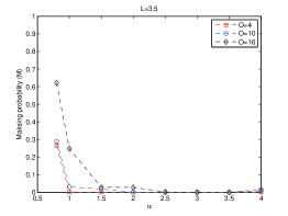
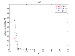
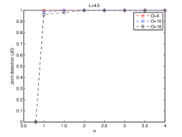
Figure 2: Masking (M) and joint detection (JD) results with respect to $\alpha$ on simulation data with different $(O$, $L)$ combinations.

7.2 Comparisons with some existing methods

We focus on the subspace estimation accuracy and compare ROC-PCA with the plain PCA and some representative robust PCA methods reviewed earlier, including RAPCA, ROBPCA, spherical PCA (S-PCA) and PCP. Note that the fast-MCD, as one of the most popular robust covariance matrix based methods, is already integrated in ROBPCA. RAPCA and ROBPCA are provided by the library LIBRA (Verboven and Hubert,, 2005). Our implementation of S-PCA follows Locantore et al., (1999). For PCP, we use the inexact augmented Lagrange multiplier algorithm (Lin et al.,, 2010). (We also tested the stable PCP and the EGMS algorithms (Zhou et al.,, 2010; Zhang and Lerman,, 2014), but they do not show better statistical performances than PCP in the presence of OC outliers, and take more time. So PCP is used as a representative method in the class of low-rank approximation based robust PCA.)

Comparison in the presence of r-Type outliers

We consider two setups with $n>p$ and $n<p$, respectively. In both setups, the data matrix ${\boldsymbol{X}}$ is generated according to Section 7.1, with $r=3$, ${\boldsymbol{D}}=\mbox{diag}\{100,60,20\}$, ${\boldsymbol{\mu}}=\boldsymbol{0}$ and $\sigma^{2}\in\{0.5,1\}$. The first $O$ rows of the outlier matrix ${\boldsymbol{S}}$ are all given by $[10,\cdots,10]$, while the rest rows are $\boldsymbol{0}$. In the $n>p$ situation, $n=100$, $p=50$, and $O\in\{4,10,16\}$. In the case of $n<p$, $n=50$, $p=100$, and $O\in\{2,5,8\}$. The major concern here is the subspace estimation accuracy and we use a conservative choice $q=2O$ for breakdown.

Table 2: PC affinity comparison in the presence of r-Type OC outliers.

$(n,p)$	$\sigma^{2}$	$O$	PCA	PCP	S-PCA	RAPCA	ROBPCA	ROC-PCA
$(100,50)$	0.5	$4$	0	6	69	51	96	96
		$10$	0	1	3	53	96	96
		$16$	0	1	1	33	95	95
	1	$4$	3	7	19	31	92	92
		$10$	1	1	3	27	92	92
		$16$	0	2	1	15	92	90
$(50,100)$	0.5	$2$	1	3	90	31	94	94
		$5$	0	2	3	21	93	93
		$8$	2	1	3	35	92	92
	1	$2$	1	2	60	21	87	87
		$5$	0	1	2	20	85	85
		$8$	1	1	1	18	84	84
$(450,15)$	0.001	$2$	0	100	100	100	1	100

Table 3: Computational time (in seconds) comparison in the presence of r-Type OC outliers.

$(n,p)$	$\sigma^{2}$	$O$	PCA	PCP	S-PCA	RAPCA	ROBPCA	ROC-PCA
$(100,50)$	0.5	$4$	0.02	0.12	0.03	0.14	1.06	5.00
		$10$	0.01	0.11	0.02	0.12	1.03	10.3
		$16$	0.01	0.11	0.02	0.12	1.08	15.9
	1	$4$	0.01	0.11	0.02	0.12	0.98	4.27
		$10$	0.01	0.11	0.02	0.12	1.01	18.2
		$16$	0.01	0.11	0.02	0.13	1.05	35.9
$(50,100)$	0.5	$2$	0.03	0.16	0.03	0.07	0.94	13.4
		$5$	0.01	0.14	0.02	0.06	0.83	20.5
		$8$	0.01	0.16	0.03	0.05	0.83	37.0
	1	$2$	0.01	0.16	0.03	0.05	0.83	10.8
		$5$	0.01	0.14	0.02	0.05	0.88	23.2
		$8$	0.01	0.15	0.02	0.05	0.81	29.9
$(450,15)$	0.001	$2$	0.05	0.05	0.04	1.19	1.15	2.63

According to the results of PCA in Table 2, the existence of OC outliers can severely skew the estimated PC directions. PCP did not show much improvement in handling OC outliers. RAPCA behaved better than PCA and PCP. But its performance deteriorates when the noise level increases. The performance of S-PCA is not stable; in particular, it showed poor results with $\geq 10\%$ outliers occurring. In contrast, ROC-PCA and ROBPCA behaved excellently in the aforementioned two setups.

To make the story complete, consider $n=450$, $p=15$, $O=2$, $\sigma^{2}=0.001$ as shown at the bottom of Table 2. In this extremely simple case, all robust PCA approaches perfectly estimated the PC subspace except ROBPCA which gave an extremely low value of PC affinity. Unfortunately, such a limitation of ROBPCA is commonly observed for datasets with large $n$, small $O$ and low $\sigma^{2}$. It is largely due to the failure of the trial direction sampling. (Indeed, in this situation most trial directions used in the multi-step ROBPCA fall into the PC subspace and so there is a large chance for outliers to remain in the $h$-subset—see Section 2.)

The computational times are reported in Table 3. ROC-PCA did not run as fast as the other procedures/algorithms, but was definitely affordable. This is an acceptable tradeoff between performance and computational complexity in robust PCA. Of course, faster algorithms are still in great need, which is an interesting topic for further research.

Comparison in the presence of e-Type outliers

To test for e-Type outliers, we generated the data under $n=100$, $p=18$, $r=3$, ${\boldsymbol{D}}=\mbox{diag}\{80,60,40\}$, ${\boldsymbol{\mu}}=\boldsymbol{0}$, $\sigma^{2}\in\{0.5,1\}$. The outlier matrix ${\boldsymbol{S}}$ has $O^{e}\in\{60,120\}$ random entries set to be $15$ and $0$ otherwise. Again, we set $q^{e}=2O^{e}$ following the discussion in Section 7.1. Table 4 and Table 5 show the mean PC affinity values and mean computational times from $50$ runs. Although ROC-PCA runs slower than the other methods, it shows superior statistical performance, especially when the number of outliers is large.

Table 4: PC affinity comparison for e-Type OC outliers.

$\sigma^{2}$	$O^{e}$	PCA	PCP	S-PCA	RAPCA	ROBPCA	ROC-PCA
0.5	$60$	16	97	98	85	80	100
	$120$	9	53	54	67	10	99
1	$60$	20	94	97	86	78	99
	$120$	9	47	48	60	10	99

Table 5: Computational time comparison for e-Type OC outliers.

$\sigma^{2}$	$O^{e}$	PCA	PCP	S-PCA	RAPCA	ROBPCA	ROC-PCA
0.5	$60$	0.03	0.03	0.03	0.16	0.99	29.5
	$120$	0.04	0.04	0.03	0.12	0.89	39.5
1	$60$	0.01	0.03	0.01	0.12	0.89	23.0
	$120$	0.02	0.04	0.03	0.12	0.90	25.4

Comparison in the presence of observation outliers

As before, we consider two types of outliers. The r-Type experiments assume the model ${\boldsymbol{X}}={\boldsymbol{L}}+{\boldsymbol{S}}+{\boldsymbol{E}}$, where ${\boldsymbol{L}}$ has rank $r$, given by ${\boldsymbol{L}}={\boldsymbol{U}}{\boldsymbol{D}}{\boldsymbol{V}}^{T}$ with randomly generated orthogonal ${\boldsymbol{U}}$ and ${\boldsymbol{V}}$, ${\boldsymbol{S}}$ is a sparse component, and ${\boldsymbol{E}}$ has i.i.d. $\mathcal{N}(0,\sigma^{2})$ entries. We set $n=100$, $p=50$, $r=3$, ${\boldsymbol{D}}=\mbox{diag}\{100,60,20\}$ and $\sigma^{2}=1$. The first $O\in\{4,10,16\}$ rows of ${\boldsymbol{S}}$ are all given by $[10,\cdots,10]$, while the rest rows are $\boldsymbol{0}$. As shown by Table 6, we found that ROC-PCA and ROBPCA usually have excellent performances. However, ROB-PCA is subject to the same trail direction sampling issue as in the r-Type OC outlier case; it can fail in very easy settings (examples not shown).

Table 6: PC affinity comparison in the presence of r-Type outliers in the observation space.

$O$	PCA	PCP	S-PCA	RAPCA	ROBPCA	ROC-PCA
$4$	14	13	41	20	92	92
$10$	10	10	15	29	91	91
$16$	11	11	13	18	90	89

The elementwise case is more complicated. Table 7 gives some examples. The experiments with e-Type outliers in the observation space use the same model, with ${\boldsymbol{U}}$ randomly generated, $n=100$, $p=18$, $r=3$, ${\boldsymbol{D}}=\mbox{diag}\{80,60,40\}$, $\sigma^{2}=1$. The following three setups are considered. 1) ${\boldsymbol{V}}$ is randomly generated and ${\boldsymbol{S}}$ has $144$ entries set to be $15$ and $0$ otherwise; 2) ${\boldsymbol{V}}={\boldsymbol{I}}[:,1:3]$ and the first three columns of the outlier matrix ${\boldsymbol{S}}$ have $12$ entries set to be $5$; 3) ${\boldsymbol{V}}$ is randomly generated and ${\boldsymbol{S}}$ has $72$ entries set to be $20$ and $0$ otherwise.

Table 7: PC affinity comparison in the presence of e-Type outliers in the observation space.

	PCA	PCP	S-PCA	RAPCA	ROBPCA	ROC-PCA
Setting 1	75	98	94	90	64	95
Setting 2	99	28	99	95	99	99
Setting 3	79	99	97	88	74	79

Most methods did not perform uniformly well. S-PCA, though simple, did a very good job. The affinity value of ROC-PCA is not very high in the last setting. A careful examination of the results shows that although checking the outlyingness in the OC subspace is reasonable, the e-Type observation outliers may lead to error propagation in the OC coordinates and so desire a much larger value of $q^{e}$. To fix this, we tried the $\ell_{0}$ penalized ROC-PCA which uses $P({\boldsymbol{S}};\lambda)=\frac{\lambda^{2}}{2}\sum 1_{s_{ij}\neq 0}$ with $\lambda$ as the threshold parameter. It falls into the $\Theta$-$P$ framework in Section 4.2 and corresponds to the hard-thresholding in implementation (She,, 2012). With $\lambda$ taken the universal threshold level $\sigma\sqrt{2\log(nd)}$ (or optimally tuned using the true PC subspace), the PC affinity value of ROC-PCA can be increased to $98$.

BROC-PCA in large-$p$ computation

We compare the standard ROC-PCA and BROC-PCA in large-$p$ setups. Data samples are generated in the same way as in Section 7.1, with $n=40$, $r=3$, ${\boldsymbol{D}}=\mbox{diag}\{80,60,40\}$, ${\boldsymbol{\mu}}=\boldsymbol{0}$ and $\sigma^{2}=1.5$. The first four rows of the outlier matrix ${\boldsymbol{S}}$ are all given by $[5,\cdots,5]$, and the remaining ones are $\boldsymbol{0}$. We vary $p$ in $\{100,300,500,1000\}$. The batch sizes we tried are described as follows: $m_{i}=35$, $i=1,2$, and $m_{3}=27$ for $p=100$; $m_{1}=100$, $m_{i}=70$, $i=2,3$, and $m_{4}=57$ for $p=300$; $m_{i}=100$, $1\leq i\leq 3$, $m_{i}=70$, $i=4,5$, $m_{6}=57$ for $p=500$; $m_{i}=100$, $1\leq i\leq 8$, $m_{i}=70$, $i=9,10$, and $m_{11}=57$ for $p=1,000$. Table 8 reports the mean CPU times (in seconds) and estimation accuracy from $20$ runs.

Table 8: Computational time and estimation accuracy for the standard ROC-PCA and BROC-PCA with different dimensions.

	ROC-PCA		BROC-PCA
	$100\cdot\cos\theta$	time	$100\cdot\cos\theta$	time
$p=100$	98	4.5	98	3.9
$p=300$	95	77.1	93	32.8
$p=500$	92	265.2	89	95.9
$p=1000$	88	2624.4	84	816.8

As show in Table 8, BROC-PCA can provide not only comparably accurate subspace recovery with the standard ROC-PCA, but impressive gains in computational efficiency as especially when $p$ is large. For example, when $p=1000$, the computational cost of the standard ROC-PCA can be reduced by almost $70\%$.

8 Real Data

We also applied ROC-PCA to analyze a segmentation dataset collected by Brodley (Lichman,, 2013) which contains features extracted from seven classes of hand-segmented images (brickface, sky, foliage, cement, window, path and grass). Each class has $330$ image regions, and for each image region $19$ features are provided (e.g., the contrast of vertically or horizontally adjacent pixels). In this experiment, we randomly picked $90$ samples from the cement class as normal observations and $10$ from the foliage class as outliers.

In PCA applications, the adjusted variance (Shen and Huang,, 2008) is often used to assess the goodness of fit. We use a robust version, called robust adjusted variance (RAV), to take outliers into account. Let $\hat{{\boldsymbol{V}}}_{r}$ be a robust estimate of the top $r$ loading vectors from data matrix ${\boldsymbol{X}}$. The RAV explained by $\hat{{\boldsymbol{V}}}_{r}$ is then defined as $\|{\boldsymbol{X}}^{0}{\boldsymbol{P}}_{\hat{{\boldsymbol{V}}}_{r}}\|_{F}^{2}/\|{{\boldsymbol{X}}}^{0}\|_{F}^{2}$, where ${{\boldsymbol{X}}}^{0}$ is a submatrix of ${\boldsymbol{X}}$ containing clean samples only.

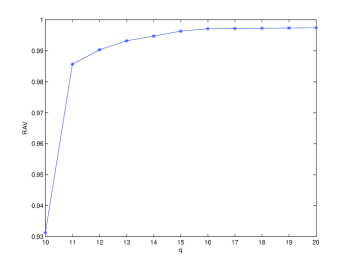
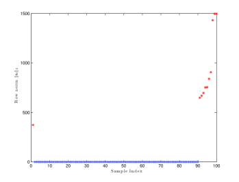
Figure 3: Left: RAV versus $q$ (with $r=3$) on the segmentation dataset. Right: Outlyingness plot: row norms of $\hat{{\boldsymbol{S}}}$. All nonzeros are marked in red. The last 10 correspond to the foliage outliers, while the first one is from the cement class.

We ran the r-Type algorithm with $r=1,2,3$ and $q$ decreasing from $20$ to $10$. Three principal components seem to be enough from the high RAV percentages in Table 9. The left panel of Figure 3 shows a relatively big drop in RAV when $q$ changes from $11$ to $10$. ROC-PCA thus yielded 11 outliers rather than 10. To get some intuition, we also plotted in the right panel the outlyingness for each observation, i.e., row norms of $\hat{{\boldsymbol{S}}}$ (with $q=11$). The last $10$ samples in the foliage class were successfully identified and most observations in the cement class have $\hat{\boldsymbol{s}}_{i}$ exactly zero. Interestingly, the first sample pops up with a large row norm of about ${400}$(!) in the outlyingness plot. We examined the data carefully and verified this finding—for example, the 7th feature for the first observation takes value 375.1, while the other $89$ samples in the same class show an average of only 1.8. The pleasant finding shows the power of ROC-PCA in automatic outlier detection without much human intervention.

We also compared ROC-PCA with PCA, PCP (Candès et al.,, 2011), S-PCA (Locantore et al.,, 1999), RAPCA (Hubert et al.,, 2002) and ROBPCA (Hubert et al.,, 2005) on the segmentation dataset. Among these methods only ROC-PCA and PCP labeled outliers explicitly. The outlying entries detected by PCP scatter all over the matrix, and the zero/nonzero pattern provides little help in separating the foliage samples from the majority of the cement data. Table 9 gives the RAV rates explained by the top $1$-$3$ PCs. The first six rows evaluated RAV on the 90 cement samples. The true performance of ROC-PCA, as shown in the last row, was assessed on the 89 clean observations in consideration of its outlier detection. The improvement bought by simultaneous subspace recovery and outlier identification is significant.

Table 9: Explained variance in terms of RAV $\times 100$, by the top $1$-$3$ PCs. The RAV evaluation of the first six rows is based on the cement class, and ROC-PCA at the bottom is after removing all its detected outliers.

	1 PC	2 PCs	3 PCs
PCA	5	20	66
PCP	13	54	57
RAPCA	45	71	80
S-PCA	48	75	81
ROBPCA	48	75	82
$\text{ROC-PCA}^{0}$	48	76	82
ROC-PCA	58	91	99

9 Conclusion

We showed that PCA is sensitive to a type of outliers which may not be easily revealed in the original observation space; mathematically formulating these projected outliers gave rise to the robust orthogonal complement PCA. We showed that ROC-PCA comes with a robust guarantee as generalized robust M-estimators, and provides ease in computation and regularization. Our theoretical analyses revealed the high breakdown point of ROC-PCA and established a non-asymptotic oracle inequality which can achieve the minimax error rate.

Some future research topics include further studies of the performance of the manifold optimization algorithm, as well as the development of faster algorithms in very high dimensions. Another interesting direction is to jointly investigate observation anomalies, which are of independent interest in many computer vision applications, and OC outliers (which can skew the PC subspace) to provide a reinforced robustification of PCP.

10 Proofs

10.1 Proof of Theorem 1

Part (i): Let $(\hat{{\boldsymbol{V}}}_{\perp},\hat{{\boldsymbol{\mu}}},\hat{{\boldsymbol{S}}})$ be a coordinate-wise minimum of the ROC-PCA problem (4) in the sense that fixing any two of $\hat{{\boldsymbol{V}}}_{\perp}$, $\hat{{\boldsymbol{\mu}}}$, and $\hat{{\boldsymbol{S}}}$, the remaining one is a (global) minimizer of (4).

The sub-problem for ${{\boldsymbol{V}}_{\perp}}$ is smooth on the Stiefel manifold. Equipped with the canonical metric, the Riemannian gradient, calculated in (10), vanishes at ${\hat{\boldsymbol{V}}}_{\perp}$. That is, ${\boldsymbol{X}}^{T}({\boldsymbol{X}}\hat{{\boldsymbol{V}}}_{\perp}-\boldsymbol{1}\hat{{\boldsymbol{\mu}}}^{T}-\hat{{\boldsymbol{S}}})=\hat{{\boldsymbol{V}}}_{\perp}({\boldsymbol{X}}\hat{{\boldsymbol{V}}}_{\perp}-\boldsymbol{1}\hat{{\boldsymbol{\mu}}}^{T}-\hat{{\boldsymbol{S}}})^{T}{\boldsymbol{X}}\hat{{\boldsymbol{V}}}_{\perp}$. The sub-problem for ${\boldsymbol{S}}$ is not necessarily convex or smooth. However, based on Lemma 1 in She, (2012), $\Theta({\boldsymbol{X}}\hat{{\boldsymbol{V}}}_{\perp}-\frac{1}{n}\boldsymbol{1}\boldsymbol{1}^{T}({\boldsymbol{X}}\hat{{\boldsymbol{V}}}_{\perp}-\hat{{\boldsymbol{S}}});\lambda)$, always gives a global minimizer for any $P$ coupled with $\Theta$ in the way of (8); see Section 4.2 in the text for details. Hence $\hat{{\boldsymbol{V}}}_{\perp}$, $\hat{{\boldsymbol{\mu}}}$ and $\hat{{\boldsymbol{S}}}$ must satisfy the following equations

$${\boldsymbol{X}}^{T}({\boldsymbol{X}}\hat{{\boldsymbol{V}}}_{\perp}-\boldsymbol{1}\hat{{\boldsymbol{\mu}}}^{T}-\hat{{\boldsymbol{S}}}) =\hat{{\boldsymbol{V}}}_{\perp}({\boldsymbol{X}}\hat{{\boldsymbol{V}}}_{\perp}-\boldsymbol{1}\hat{{\boldsymbol{\mu}}}^{T}-\hat{{\boldsymbol{S}}})^{T}{\boldsymbol{X}}\hat{{\boldsymbol{V}}}_{\perp},$$ (18)

$$\hat{{\boldsymbol{S}}} =\Theta({\boldsymbol{X}}\hat{{\boldsymbol{V}}}_{\perp}-\frac{1}{n}\boldsymbol{1}\boldsymbol{1}^{T}({\boldsymbol{X}}\hat{{\boldsymbol{V}}}_{\perp}-\hat{{\boldsymbol{S}}});\lambda),$$ (19)

$$\hat{{\boldsymbol{\mu}}} =\frac{1}{n}({\boldsymbol{X}}\hat{{\boldsymbol{V}}}_{\perp}-\hat{\boldsymbol{S}})^{T}\boldsymbol{1}.$$ (20)

Now, for $\psi(t)=t-\Theta(t;\lambda)$, we have

$$\begin{array}[]{ll}&\psi({\boldsymbol{X}}\hat{{\boldsymbol{V}}}_{\perp}-\boldsymbol{1}\hat{{\boldsymbol{\mu}}}^{T};\lambda)\\ =&{\boldsymbol{X}}\hat{{\boldsymbol{V}}}_{\perp}-\boldsymbol{1}\hat{{\boldsymbol{\mu}}}^{T}-\Theta({\boldsymbol{X}}\hat{{\boldsymbol{V}}}_{\perp}-\boldsymbol{1}\hat{{\boldsymbol{\mu}}}^{T};\lambda)\\ =&{\boldsymbol{X}}\hat{{\boldsymbol{V}}}_{\perp}-\boldsymbol{1}\hat{{\boldsymbol{\mu}}}^{T}-\Theta({\boldsymbol{X}}\hat{{\boldsymbol{V}}}_{\perp}-\frac{1}{n}\boldsymbol{1}\boldsymbol{1}^{T}({\boldsymbol{X}}\hat{{\boldsymbol{V}}}_{\perp}-\hat{{\boldsymbol{S}}});\lambda)\\ =&{\boldsymbol{X}}\hat{{\boldsymbol{V}}}_{\perp}-\boldsymbol{1}\hat{{\boldsymbol{\mu}}}^{T}-\hat{\boldsymbol{S}},\end{array}$$

where the last two equalities are by (20) and (19), respectively. It follows that

$$\begin{array}[]{ll}&{\boldsymbol{X}}^{T}\psi({\boldsymbol{X}}\hat{{\boldsymbol{V}}}_{\perp}-\boldsymbol{1}{\boldsymbol{\mu}}^{T};\lambda)-\hat{{\boldsymbol{V}}}_{\perp}(\psi({\boldsymbol{X}}{{\boldsymbol{V}}_{\perp}}-\boldsymbol{1}{\boldsymbol{\mu}}^{T};\lambda))^{T}{\boldsymbol{X}}\hat{{\boldsymbol{V}}}_{\perp}\\ =&{\boldsymbol{X}}^{T}({\boldsymbol{X}}\hat{{\boldsymbol{V}}}_{\perp}-\boldsymbol{1}\hat{{\boldsymbol{\mu}}}^{T}-\hat{{\boldsymbol{S}}})-\hat{{\boldsymbol{V}}}_{\perp}({\boldsymbol{X}}\hat{{\boldsymbol{V}}}_{\perp}-\boldsymbol{1}\hat{{\boldsymbol{\mu}}}^{T}-\hat{{\boldsymbol{S}}})^{T}{\boldsymbol{X}}\hat{{\boldsymbol{V}}}_{\perp}\\ =&\boldsymbol{0},\end{array}$$

with the last equality due to (18). Moreover, we have

$$\begin{array}[]{ll}&\boldsymbol{1}^{T}\psi({\boldsymbol{X}}\hat{{\boldsymbol{V}}}_{\perp}-\boldsymbol{1}\hat{{\boldsymbol{\mu}}}^{T};\lambda)\\ =&\boldsymbol{1}^{T}\psi({\boldsymbol{X}}\hat{{\boldsymbol{V}}}_{\perp}-\frac{1}{n}\boldsymbol{1}\boldsymbol{1}^{T}({\boldsymbol{X}}\hat{{\boldsymbol{V}}}_{\perp}-\hat{{\boldsymbol{S}}});\lambda)\ \ \mbox{(by \eqref{eq:coordminimum3})}\\ =&\boldsymbol{1}^{T}({\boldsymbol{X}}\hat{{\boldsymbol{V}}}_{\perp}-\frac{1}{n}\boldsymbol{1}\boldsymbol{1}^{T}({\boldsymbol{X}}\hat{{\boldsymbol{V}}}_{\perp}-\hat{{\boldsymbol{S}}})-\Theta({\boldsymbol{X}}\hat{{\boldsymbol{V}}}_{\perp}-\frac{1}{n}\boldsymbol{1}\boldsymbol{1}^{T}({\boldsymbol{X}}\hat{{\boldsymbol{V}}}_{\perp}-\hat{{\boldsymbol{S}}});\lambda))\\ =&\boldsymbol{1}^{T}({\boldsymbol{X}}\hat{{\boldsymbol{V}}}_{\perp}-\frac{1}{n}\boldsymbol{1}\boldsymbol{1}^{T}({\boldsymbol{X}}\hat{{\boldsymbol{V}}}_{\perp}-\hat{{\boldsymbol{S}}})-\hat{{\boldsymbol{S}}})\ \mbox{(by \eqref{eq:coordminimum2})}\\ =&\boldsymbol{1}^{T}({\boldsymbol{I}}-\frac{1}{n}\boldsymbol{1}\boldsymbol{1}^{T}){\boldsymbol{X}}\hat{{\boldsymbol{V}}}_{\perp}\\ =&\boldsymbol{0}.\end{array}$$

Therefore, $(\hat{{\boldsymbol{V}}}_{\perp},\hat{{\boldsymbol{\mu}}})$ is also an $M$-estimate associated with $\psi$.

Part (ii): The proof is straightforward and the details are omitted.

10.2 Proof of Theorem 2

Throughout this proof, we use $C$, $c$, $L$ to denote universal constants. They are not necessarily the same at each occurrence.

Given any matrix ${\boldsymbol{A}}$, we use $CS({\boldsymbol{A}})$ and $RS({\boldsymbol{A}})$ to denote its column space and row space, respectively, and ${\mathbf{P}}_{{\boldsymbol{A}}}$ to denote the orthogonal projection matrix onto $CS({\boldsymbol{A}})$, i.e., ${\mathbf{P}}_{{\boldsymbol{A}}}={\boldsymbol{A}}({\boldsymbol{A}}^{T}{\boldsymbol{A}})^{+}{\boldsymbol{A}}^{T}$, where ⁺ stands for the Moore-Penrose pseudoinverse, while ${\mathbf{P}}_{{\boldsymbol{A}}}^{\perp}$ denotes the projection onto the orthogonal complement of $CS({\boldsymbol{A}})$. We also use such projection matrices to denote the associated subspaces by a bit abuse of notation. Given two matrices ${\boldsymbol{A}}$ and ${\boldsymbol{B}}$ of the same dimensions, their inner product is defined as $\langle{\boldsymbol{A}},{\boldsymbol{B}}\rangle=tr({\boldsymbol{A}}^{T}{\boldsymbol{B}})$.

First, by the definition of ROC-PCA, we have

$$\begin{split}&\frac{np}{2}M(\hat{\boldsymbol{A}},\hat{\boldsymbol{S}},\hat{\boldsymbol{V}},\hat{\boldsymbol{V}}_{\perp};{\boldsymbol{A}}^{*},{\boldsymbol{S}}^{*},{\boldsymbol{V}}^{*},{\boldsymbol{V}}_{\perp}^{*})\\ \leq&\ \frac{np}{2}M({\boldsymbol{A}},{\boldsymbol{S}},{\boldsymbol{V}},{\boldsymbol{V}}_{\perp};{\boldsymbol{A}}^{*},{\boldsymbol{S}}^{*},{\boldsymbol{V}}^{*},{\boldsymbol{V}}_{\perp}^{*})+\langle{\boldsymbol{E}},\hat{\boldsymbol{A}}\hat{\boldsymbol{V}}^{T}+\hat{\boldsymbol{S}}\hat{\boldsymbol{V}}_{\perp}^{T}-{\boldsymbol{A}}{\boldsymbol{V}}^{T}-{\boldsymbol{S}}{\boldsymbol{V}}_{\perp}^{T}\rangle.\end{split}$$ (21)

Define $\mathcal{J}=\{i:{\boldsymbol{S}}[i,:]\neq\boldsymbol{0}\}$, $\hat{\mathcal{J}}=\{i:\hat{\boldsymbol{S}}[i,:]\neq\boldsymbol{0}\}$, and $\tilde{\mathcal{J}}=\mathcal{J}\cup\hat{\mathcal{J}}$. For convenience, we denote ${\mathbf{P}}_{{\boldsymbol{I}}[:,\tilde{\mathcal{J}}]}$ by ${\mathbf{P}}_{\tilde{\mathcal{J}}}$ and its orthogonal complement by ${\mathbf{P}}_{\tilde{\mathcal{J}}}^{\perp}$; ${\mathbf{P}}_{\hat{\mathcal{J}}}$, ${\mathbf{P}}_{{\mathcal{J}}}$ and ${\mathbf{P}}_{{\mathcal{J}}}^{\perp}$ are defined similarly. Then

$$\hat{\boldsymbol{A}}\hat{\boldsymbol{V}}^{T}+\hat{\boldsymbol{S}}\hat{\boldsymbol{V}}_{\perp}^{T}-{\boldsymbol{A}}{\boldsymbol{V}}^{T}-{\boldsymbol{S}}{\boldsymbol{V}}_{\perp}^{T}$$

$$= (\hat{\boldsymbol{A}}\hat{\boldsymbol{V}}^{T}+\hat{\boldsymbol{S}}\hat{\boldsymbol{V}}_{\perp}^{T}-{\boldsymbol{A}}{\boldsymbol{V}}^{T}){\mathbf{P}}_{{\boldsymbol{V}}}+{\mathbf{P}}_{\tilde{\mathcal{J}}}^{\perp}\hat{\boldsymbol{A}}\hat{\boldsymbol{V}}^{T}{\mathbf{P}}_{{\boldsymbol{V}}_{\perp}}+{\mathbf{P}}_{\tilde{\mathcal{J}}}(\hat{\boldsymbol{A}}\hat{\boldsymbol{V}}^{T}+\hat{\boldsymbol{S}}\hat{\boldsymbol{V}}_{\perp}^{T}-{\boldsymbol{S}}{\boldsymbol{V}}_{\perp}^{T}){\mathbf{P}}_{{\boldsymbol{V}}_{\perp}}$$

$$= (\hat{\boldsymbol{A}}\hat{\boldsymbol{V}}^{T}+\hat{\boldsymbol{S}}\hat{\boldsymbol{V}}_{\perp}^{T}-{\boldsymbol{A}}{\boldsymbol{V}}^{T}){\mathbf{P}}_{{\boldsymbol{V}}}+{\mathbf{P}}_{\tilde{\mathcal{J}}}^{\perp}\hat{\boldsymbol{A}}\hat{\boldsymbol{V}}^{T}{\mathbf{P}}_{{\boldsymbol{V}}_{\perp}}+({\mathbf{P}}_{{\mathcal{J}}}\cap{\mathbf{P}}_{\tilde{\mathcal{J}}})(\hat{\boldsymbol{A}}\hat{\boldsymbol{V}}^{T}+\hat{\boldsymbol{S}}\hat{\boldsymbol{V}}_{\perp}^{T}-{\boldsymbol{S}}{\boldsymbol{V}}_{\perp}^{T}){\mathbf{P}}_{{\boldsymbol{V}}_{\perp}}$$

$$+({\mathbf{P}}_{\mathcal{J}}^{\perp}\cap{\mathbf{P}}_{\tilde{\mathcal{J}}})(\hat{\boldsymbol{A}}\hat{\boldsymbol{V}}^{T}+\hat{\boldsymbol{S}}\hat{\boldsymbol{V}}_{\perp}^{T}-{\boldsymbol{S}}{\boldsymbol{V}}_{\perp}^{T}){\mathbf{P}}_{{\boldsymbol{V}}_{\perp}}$$

$$= (\hat{\boldsymbol{A}}\hat{\boldsymbol{V}}^{T}+\hat{\boldsymbol{S}}\hat{\boldsymbol{V}}_{\perp}^{T}-{\boldsymbol{A}}{\boldsymbol{V}}^{T}){\mathbf{P}}_{{\boldsymbol{V}}}+{\mathbf{P}}_{\tilde{\mathcal{J}}}^{\perp}\hat{\boldsymbol{A}}\hat{\boldsymbol{V}}^{T}{\mathbf{P}}_{{\boldsymbol{V}}_{\perp}}+{\mathbf{P}}_{{\mathcal{J}}}(\hat{\boldsymbol{A}}\hat{\boldsymbol{V}}^{T}+\hat{\boldsymbol{S}}\hat{\boldsymbol{V}}_{\perp}^{T}-{\boldsymbol{S}}{\boldsymbol{V}}_{\perp}^{T}){\mathbf{P}}_{{\boldsymbol{V}}_{\perp}}$$

$$+({\mathbf{P}}_{\mathcal{J}}^{\perp}\cap{\mathbf{P}}_{\hat{\mathcal{J}}})(\hat{\boldsymbol{A}}\hat{\boldsymbol{V}}^{T}+\hat{\boldsymbol{S}}\hat{\boldsymbol{V}}_{\perp}^{T}-{\boldsymbol{S}}{\boldsymbol{V}}_{\perp}^{T}){\mathbf{P}}_{{\boldsymbol{V}}_{\perp}}$$

$$\equiv {\boldsymbol{C}}_{1}+{\boldsymbol{C}}_{2}+{\boldsymbol{C}}_{3}+{\boldsymbol{C}}_{4}.$$

Clearly, $rank({\boldsymbol{C}}_{1})\leq rank({\mathbf{P}}_{{\boldsymbol{V}}})=r$, $rank({\boldsymbol{C}}_{2})\leq rank(\hat{\boldsymbol{V}})=r$, $rank({\boldsymbol{C}}_{3})\leq rank({\mathbf{P}}_{{\mathcal{J}}})\leq q$, $rank({\boldsymbol{C}}_{4})\leq rank({\mathbf{P}}_{\mathcal{J}}^{\perp}\cap{\mathbf{P}}_{\hat{\mathcal{J}}})\leq q$. Due to the orthogonality between ${\boldsymbol{C}}_{1}$, ${\boldsymbol{C}}_{2}$, ${\boldsymbol{C}}_{3}$, and ${\boldsymbol{C}}_{4}$, $\|\hat{\boldsymbol{A}}\hat{\boldsymbol{V}}^{T}+\hat{\boldsymbol{S}}\hat{\boldsymbol{V}}_{\perp}^{T}-{\boldsymbol{A}}{\boldsymbol{V}}^{T}-{\boldsymbol{S}}{\boldsymbol{V}}_{\perp}^{T}\|_{F}^{2}=\sum_{l=1}^{4}\|{\boldsymbol{C}}_{l}\|_{F}^{2}$. The last term of (21) now becomes

$$\langle{\boldsymbol{E}}, \hat{\boldsymbol{A}}\hat{\boldsymbol{V}}^{T}+\hat{\boldsymbol{S}}\hat{\boldsymbol{V}}_{\perp}^{T}-{\boldsymbol{A}}{\boldsymbol{V}}^{T}-{\boldsymbol{S}}{\boldsymbol{V}}_{\perp}^{T}\rangle=\sum_{l=1}^{4}\langle{\boldsymbol{E}},{\boldsymbol{C}}_{l}\rangle.$$ (22)

A lemma will be introduced to bound each term on the right. To make our conclusion more general, we only require that ${\boldsymbol{E}}$ is sub-Gaussian.

Definition 1.

$\xi$ is called a sub-Gaussian random variable if there exist constants $C,c>0$ such that $\,\mathbb{P}\{|\xi|\geq t\}\leq Ce^{-ct^{2}},\forall t>0$. The scale ($\psi_{2}$-norm) for $\xi$ is defined as $\sigma(\xi)=\inf\{\sigma>0:\,\mathbb{E}\exp(\xi^{2}/\sigma^{2})\leq 2\}$. ${\boldsymbol{\xi}}\in\mathbb{R}^{p}$ is called a sub-Gaussian random vector with scale bounded by $\sigma$ if all one-dimensional marginals $\langle{\boldsymbol{\xi}},{\boldsymbol{\alpha}}\rangle$ are sub-Gaussian satisfying $\|\langle{\boldsymbol{\xi}},{\boldsymbol{\alpha}}\rangle\|_{\psi_{2}}\leq\sigma\|{\boldsymbol{\alpha}}\|_{2}$, $\forall{\boldsymbol{\alpha}}\in R^{p}$.

Some examples include Gaussian random variables and bounded random variables (such as Bernoulli). The following lemma assumes $\operatorname{\mbox{vec}\,}({\boldsymbol{E}})$ is sub-Gaussian.

Lemma 1.

Suppose ${\boldsymbol{E}}\in\mathbb{R}^{n\times m}$ and $\operatorname{\mbox{vec}\,}({\boldsymbol{E}})$ is sub-Gaussian with mean zero and $\psi_{2}$-norm bounded by $\sigma$. (i) Given ${\boldsymbol{X}}\in\mathbb{R}^{n\times p}$, $1\leq J\leq p$, $1\leq r\leq J\wedge m$, define $\Gamma_{J,r}^{{\boldsymbol{X}}}=\{{\boldsymbol{A}}\in\mathbb{R}^{n\times m}:\|{\boldsymbol{A}}\|_{F}\leq 1,\mbox{rank}({\boldsymbol{A}})\leq r,CS({\boldsymbol{A}})\subset{\mathbf{P}}_{{\boldsymbol{X}}_{\mathcal{J}}})\mbox{ for some }\mathcal{J}:|\mathcal{J}|=J\}$ with ${\boldsymbol{X}}_{\mathcal{J}}$ denoting the submatrix consisting of the columns of ${\boldsymbol{X}}$ indexed by $\mathcal{J}$. Let $P_{o}^{\prime}(J,r)=\sigma^{2}\{[\mbox{rank}({\boldsymbol{X}})\wedge J+m-r]r+\log{p\choose J}\}$. Then for any $t\geq 0$,

$$\,\mathbb{P}\left(\sup_{{\boldsymbol{A}}\in\Gamma_{J,r}^{{\boldsymbol{X}}}}\langle{\boldsymbol{E}},{\boldsymbol{A}}\rangle\geq t\sigma+\sqrt{L\cdot P_{o}^{\prime}(J,r)}\right)\leq C\exp(-ct^{2}),$$ (23)

where $L,C,c>0$ are universal constants. (ii) Given ${\boldsymbol{X}}\in\mathbb{R}^{n\times p}$, $1\leq J,J^{\prime}\leq p$, $1\leq r\leq J\wedge m$, define $\Gamma_{J,J^{\prime},r}^{{\boldsymbol{X}}}=\{{\boldsymbol{A}}\in\mathbb{R}^{n\times m}:\|{\boldsymbol{A}}\|_{F}\leq 1,rank({\boldsymbol{A}})\leq r,CS({\boldsymbol{A}})\subset{\mathbf{P}}_{{\boldsymbol{X}}_{\mathcal{J}}}^{\perp}\cap{\mathbf{P}}_{{\boldsymbol{X}}_{\mathcal{J}^{\prime}}}\mbox{ for some }{\mathcal{J}},{\mathcal{J}}^{\prime}\subset[p]\mbox{ satisfying }|{\mathcal{J}}^{\prime}|=J^{\prime},|{\mathcal{J}}|=J\}$. Let $P_{o}^{\prime\prime}(J,J^{\prime},r)=\sigma^{2}\{(rank({\boldsymbol{X}})\wedge J^{\prime}\wedge(p-J))r+(m-r)r+\log{p\choose J}+\log{p\choose J^{\prime}}\}$. Then for any $t\geq 0$,

$$\,\mathbb{P}\left(\sup_{{\boldsymbol{A}}\in\Gamma_{J,J^{\prime},r}^{{\boldsymbol{X}}}}\langle{\boldsymbol{E}},{\boldsymbol{A}}\rangle\geq t\sigma+\sqrt{L\cdot P_{o}^{\prime\prime}(J,J^{\prime},r)}\right)\leq C\exp(-ct^{2}),$$ (24)

where $L,C,c>0$ are universal constants.

The proof of the lemma follows similar lines of the proof of Lemma 4 in She, (2014) and is omitted.

Noticing that ${\boldsymbol{C}}_{1},{\boldsymbol{C}}_{2}\in\Gamma_{n,r}^{{\boldsymbol{I}}}$, ${\boldsymbol{C}}_{3}\in\Gamma_{q,d}^{{\boldsymbol{I}}}$, ${\boldsymbol{C}}_{4}\in\Gamma_{q,q,d}^{{\boldsymbol{I}}}$, we can apply the lemma to bound (22). Take ${\boldsymbol{C}}_{3}$ as an example. Letting $P_{o}^{(3)}(q,d)=\sigma^{2}\{qd+(p-d)d+\log{n\choose q}\}$, we have $\langle{\boldsymbol{E}},{\boldsymbol{C}}_{3}\rangle-\frac{1}{a}\|{\boldsymbol{C}}_{3}\|_{F}^{2}-bLP_{o}^{(3)}(q,d)\leq\|{\boldsymbol{C}}_{3}\|_{F}\langle{\boldsymbol{E}},{\boldsymbol{C}}_{3}/\|{\boldsymbol{C}}_{3}\|_{F}\rangle-2\sqrt{\frac{b}{a}}\|{\boldsymbol{C}}_{3}\|_{F}\sqrt{LP_{o}^{(3)}(q,d)}$, which is further bounded by $\frac{1}{a^{\prime}}\|{\boldsymbol{C}}_{3}\|_{F}^{2}+\frac{a^{\prime}}{4}\sup_{1\leq q\leq n,1\leq d\leq p}\left(\sup_{{\boldsymbol{A}}\in\Gamma_{q,d}^{{\boldsymbol{I}}}}\langle{\boldsymbol{E}},{\boldsymbol{A}}\rangle-2\sqrt{\frac{b}{a}}\sqrt{LP_{o}^{(3)}(q,d)}\right)_{+}^{2}$ for any $a,b,a^{\prime}>0$. Denote the last term by $\frac{a^{\prime}}{4}R^{2}$ with $R^{2}=\sup_{1\leq q\leq n,1\leq d\leq p}R_{q,d}$. From Part (i) of Lemma 1, $\,\mathbb{E}R^{2}\leq C\sigma^{2}$ if we choose $b>4a$. Indeed,

$$\quad\,\mathbb{P}(R\geq t\sigma)$$

$$\leq\sum_{q=1}^{n}\sum_{d=1}^{p}\,\mathbb{P}(R_{q,d}\geq t\sigma)$$

$$\leq\sum_{q=1}^{n}\sum_{d=1}^{p}\,\mathbb{P}(\sup_{{\boldsymbol{A}}\in\Gamma_{q,d}^{{\boldsymbol{I}}}}\langle{\boldsymbol{E}},{\boldsymbol{A}}\rangle-\sqrt{LP_{o}^{(3)}(q,d)}\geq t\sigma+(2\sqrt{{b}/{a}}-1)\sqrt{LP_{o}^{(3)}(q,d)})$$

$$\leq\sum_{q=1}^{n}\sum_{d=1}^{p}C\exp(-ct^{2})\exp\left\{-c\left((2\sqrt{{b}/{a}}-1)^{2}L\cdot P_{o}^{(3)}(q,d)/\sigma^{2}\right)\right\}\leq C^{\prime}\exp(-ct^{2}).$$

The other terms $\langle{\boldsymbol{E}},{\boldsymbol{C}}_{1}\rangle,\langle{\boldsymbol{E}},{\boldsymbol{C}}_{2}\rangle$, and $\langle{\boldsymbol{E}},{\boldsymbol{C}}_{4}\rangle$ can be similarly handled by Lemma 1.

In summary, letting we obtain a bound for (22) as follows

$$\,\mathbb{E}\langle{\boldsymbol{E}},\hat{\boldsymbol{A}}\hat{\boldsymbol{V}}^{T}+\hat{\boldsymbol{S}}\hat{\boldsymbol{V}}_{\perp}^{T}-{\boldsymbol{A}}{\boldsymbol{V}}^{T}-{\boldsymbol{S}}{\boldsymbol{V}}_{\perp}^{T}\rangle$$

$$\leq \,\mathbb{E}\{(\frac{1}{a}+\frac{1}{a^{\prime}})\|\hat{\boldsymbol{A}}\hat{\boldsymbol{V}}^{T}+\hat{\boldsymbol{S}}\hat{\boldsymbol{V}}_{\perp}^{T}-{\boldsymbol{A}}{\boldsymbol{V}}^{T}-{\boldsymbol{S}}{\boldsymbol{V}}_{\perp}^{T}\|_{F}^{2}\}+C\sigma^{2}+$$

$$+bL\sigma^{2}\{2nr+2(p-r)r+qd+(p-d)d+qd+(p-d)d+3\log{n\choose J}\}$$

$$\leq \,\mathbb{E}\{(\frac{1}{a}+\frac{1}{a^{\prime}})(1+b^{\prime})\|{\boldsymbol{A}}{\boldsymbol{V}}^{T}+{\boldsymbol{S}}{\boldsymbol{V}}_{\perp}^{T}-{\boldsymbol{A}}^{*}{\boldsymbol{V}}^{*T}-{\boldsymbol{S}}^{*}{\boldsymbol{V}}_{\perp}^{*T}\|_{F}^{2}$$

$$+(\frac{1}{a}+\frac{1}{a^{\prime}})(1+\frac{1}{b^{\prime}})\|\hat{\boldsymbol{A}}\hat{\boldsymbol{V}}^{T}+\hat{\boldsymbol{S}}\hat{\boldsymbol{V}}_{\perp}^{T}-{\boldsymbol{A}}^{*}{\boldsymbol{V}}^{*T}-{\boldsymbol{S}}^{*}{\boldsymbol{V}}_{\perp}^{*T}\|_{F}^{2}\}$$

$$+bCL\sigma^{2}\{qp+pr+nr+q\log(en/q)\},$$

for any $a,b,a^{\prime},b^{\prime}$ that are positive and satisfy $b>4a$. Choosing $(\frac{1}{a}+\frac{1}{a^{\prime}})(1+\frac{1}{b^{\prime}})<\frac{1}{2}$ and $b>4a$ (e.g., $a=a^{\prime}=8$, $b^{\prime}=2$, $b=33$), we get $np\,\mathbb{E}M(\hat{\boldsymbol{A}},\hat{\boldsymbol{S}},\hat{\boldsymbol{V}},\hat{\boldsymbol{V}}_{\perp};{\boldsymbol{A}}^{*},{\boldsymbol{S}}^{*},{\boldsymbol{V}}^{*},{\boldsymbol{V}}_{\perp}^{*})\leq CnpM({\boldsymbol{A}},{\boldsymbol{S}},{\boldsymbol{V}},{\boldsymbol{V}}_{\perp};{\boldsymbol{A}}^{*},{\boldsymbol{S}}^{*},{\boldsymbol{V}}^{*},{\boldsymbol{V}}_{\perp}^{*})+C\sigma^{2}+npP_{o}(q,r;n,p,\sigma^{2}).$

10.3 Proof of Theorem 3

Let ${\boldsymbol{B}}({\boldsymbol{A}},{\boldsymbol{S}},{\boldsymbol{V}},{\boldsymbol{V}}_{\perp})={\boldsymbol{A}}{\boldsymbol{V}}^{T}+{\boldsymbol{S}}{\boldsymbol{V}}_{\perp}^{T}$. With a bit abuse of notation, the set of ${\boldsymbol{B}}({\boldsymbol{A}},{\boldsymbol{S}},{\boldsymbol{V}},{\boldsymbol{V}}_{\perp})$ for all $({\boldsymbol{A}},{\boldsymbol{S}},{\boldsymbol{V}},{\boldsymbol{V}}_{\perp})\in\mathcal{S}(r,q)$ is still denoted by $\mathcal{S}(r,q)$.

Case (i) $(n+p)r<qd+q\log(en/q)$. Define a signal subclass ${\mathcal{B}}^{1}(r,q)=\{{\boldsymbol{B}}({\boldsymbol{A}},{\boldsymbol{S}},{\boldsymbol{V}},{\boldsymbol{V}}_{\perp}):{\boldsymbol{A}}=\boldsymbol{0},{\boldsymbol{S}}\in{\mathcal{B}}_{S}^{1}(r,q),{\boldsymbol{V}}={\boldsymbol{I}}[:,1:r],{\boldsymbol{V}}_{\perp}={\boldsymbol{I}}[:,(r+1):p]\}$, where

$${\mathcal{B}}_{S}^{1}(r,q) =\{{\boldsymbol{S}}\in\mathbb{R}^{n\times d}:{\boldsymbol{S}}=[{\boldsymbol{S}}^{l},{\boldsymbol{S}}^{r}],{\boldsymbol{S}}^{l}=[{\boldsymbol{s}}_{1}^{l},\ldots,{\boldsymbol{s}}_{n}^{l}]^{T}\in\mathbb{R}^{n\times[d/2]}\mbox{ with }{\boldsymbol{s}}_{i}^{l}\in\{\boldsymbol{0},\gamma R\cdot\boldsymbol{1}\},$$

$${\boldsymbol{S}}^{r}=[s_{i,j}^{r}]\in\mathbb{R}^{n\times(d-[d/2])},s_{i,j}^{r}=0\mbox{ if }{\boldsymbol{s}}_{i}^{l}=\boldsymbol{0},\mbox{ and }\in\{0,\gamma R\}\mbox{ otherwise},\mbox{ and }\|{\boldsymbol{S}}\|_{2,0}\leq q\}.$$

Here $R={\sigma}(1+\frac{\log(en/q)}{d})^{1/2}$ and $\gamma>0$ is a small constant to be chosen later. Clearly, ${\mathcal{B}}^{1}(r,q)\subset\mathcal{S}(r,q)$. By Stirling’s approximation, $\log|\mathcal{B}^{1}(q)|\geq\log{n\choose q}+\log 2^{qd/2}\geq q\log(n/q)+(qd/2)\log 2\geq c\{q\log(en/q)+qd\}$ for some universal constant $c$. Let $\rho({\boldsymbol{S}}_{1},{\boldsymbol{S}}_{2})=\|\operatorname{\mbox{vec}\,}({\boldsymbol{S}}_{1})-\operatorname{\mbox{vec}\,}({\boldsymbol{S}}_{2})\|_{0}$ be the Hamming distance. Applying Lemma 8.3 of Rigollet and Tsybakov, (2011) row-wise, followed by the Varshamov-Gilbert bound (cf. Lemma 2.9 in Tsybakov, (2009)), there exists a subset ${\mathcal{B}}_{S}^{10}(r,q)\subset{\mathcal{B}}_{S}^{1}(r,q)$ such that

$$\log|{\mathcal{B}}_{S}^{10}(r,q)|\geq c_{1}(q\log(en/q)+qd)\mbox{ and }\rho({\boldsymbol{S}}_{1},{\boldsymbol{S}}_{2})\geq c_{2}qd,\forall{\boldsymbol{S}}_{1},{\boldsymbol{S}}_{2}\in{\mathcal{B}}_{S}^{10},{\boldsymbol{S}}_{1}\neq{\boldsymbol{S}}_{2}$$ (25)

for some universal constants $c_{1},c_{2}>0$. Let ${\mathcal{B}}^{10}(r,q)=\{{\boldsymbol{B}}({\boldsymbol{A}},{\boldsymbol{S}},{\boldsymbol{V}},{\boldsymbol{V}}_{\perp}):{\boldsymbol{A}}=\boldsymbol{0},{\boldsymbol{S}}\in{\mathcal{B}}_{S}^{10}(r,q),{\boldsymbol{V}}={\boldsymbol{I}}[:,1:r],{\boldsymbol{V}}_{\perp}={\boldsymbol{I}}[:,(r+1):p]\}$. Then for any ${\boldsymbol{B}}_{1},{\boldsymbol{B}}_{2}\in\mathcal{B}^{10}(r,q)$, ${\boldsymbol{B}}_{1}\neq{\boldsymbol{B}}_{2}$,

$$\|{\boldsymbol{B}}_{1}-{\boldsymbol{B}}_{2}\|_{F}^{2}=\gamma^{2}R^{2}\rho({\boldsymbol{B}}_{1},{\boldsymbol{B}}_{2})\geq c_{2}\gamma^{2}R^{2}qd.$$ (26)

For Gaussian models, the Kullback-Leibler divergence of $\mathcal{MN}({\boldsymbol{B}}_{2},\sigma^{2}\boldsymbol{I}\otimes{\boldsymbol{I}})$ (denoted by $P_{{\boldsymbol{B}}_{2}}$) from $\mathcal{MN}({\boldsymbol{B}}_{1},\sigma^{2}\boldsymbol{I}\otimes{\boldsymbol{I}})$ (denoted by $P_{{\boldsymbol{B}}_{1}}$) is $\mathcal{K}(\mathcal{P}_{{\boldsymbol{B}}_{1}},\mathcal{P}_{{\boldsymbol{B}}_{2}})=\frac{1}{2\sigma^{2}}\|{\boldsymbol{B}}_{1}-{\boldsymbol{B}}_{2}\|_{F}^{2}$. Let $P_{\boldsymbol{0}}$ be $\mathcal{MN}(\boldsymbol{0},\sigma^{2}\boldsymbol{I}\otimes{\boldsymbol{I}})$. Then, for any ${\boldsymbol{B}}\in{\mathcal{B}}^{1}(r,q)$, we have

$$\mathcal{K}(P_{\boldsymbol{0}},P_{{\boldsymbol{B}}})=\frac{1}{2\sigma^{2}}\|\boldsymbol{0}-{\boldsymbol{S}}\|_{F}^{2}\leq\frac{\gamma^{2}}{\sigma^{2}}R^{2}qd$$

and so

$$\frac{1}{|\mathcal{B}^{10}|}\sum_{{\boldsymbol{B}}\in\mathcal{B}^{10}(r,q)}\mathcal{K}(P_{\boldsymbol{0}},P_{{\boldsymbol{B}}})\leq\gamma^{2}(qd+q\log(en/q)).$$ (27)

Combining (26) and (27) and choosing a sufficiently small value for $\gamma$, we can apply Theorem 2.7 of Tsybakov, (2009) to get the desired lower bound.

Case (ii) $(n+p)r\geq qd+q\log(en/q)$. Consider a signal subclass

$${\mathcal{B}}^{2}(r)=\{{\boldsymbol{B}}=[b_{i,j}]\in\mathbb{R}^{n\times p}: \ b_{i,j}=0\mbox{ or }\gamma\sigma\mbox{ if }(i,j)\in[n]\times[r/2]\cup[r/2]\times[p]$$

$$\mbox{ and }b_{i,j}=0\mbox{ otherwise}\}.$$

where $\gamma>0$ is a small constant to be chosen later. Then it is not difficult to see that $|{\mathcal{B}}^{2}(r)|=2^{(n+p-r/2)r}$, $\mathcal{B}^{2}(r)\subset\mathcal{B}(r,q)$, and $r({\boldsymbol{B}}_{1}-{\boldsymbol{B}}_{2})\leq r$, $\forall{\boldsymbol{B}}_{1},{\boldsymbol{B}}_{2}\in\mathcal{B}^{2}(r)$. Also, since $r\leq n\wedge p$, $(n+p-r/2)r\geq c(n+p)r$ for some universal constant $c$.

Let $\rho({\boldsymbol{B}}_{1},{\boldsymbol{B}}_{2})=\|\operatorname{\mbox{vec}\,}({\boldsymbol{B}}_{1})-\operatorname{\mbox{vec}\,}({\boldsymbol{B}}_{2})\|_{0}$ be the Hamming distance. By the Varshamov-Gilbert bound, there exists a subset ${\mathcal{B}}^{20}(r)\subset{\mathcal{B}}^{2}(r)$ such that

$$\log|{\mathcal{B}}^{20}(r)|\geq c_{1}r(n+p),\mbox{ and }\rho({\boldsymbol{B}}_{1},{\boldsymbol{B}}_{2})\geq c_{2}r(n+p),\forall{\boldsymbol{B}}_{1},{\boldsymbol{B}}_{2}\in\mathcal{B}^{20},{\boldsymbol{B}}_{1}\neq{\boldsymbol{B}}_{2}$$

for some universal constants $c_{1},c_{2}>0$. Therefore, $\|{\boldsymbol{B}}_{1}-{\boldsymbol{B}}_{2}\|_{F}^{2}=\gamma^{2}\sigma^{2}\rho({\boldsymbol{B}}_{1},{\boldsymbol{B}}_{2})\geq c_{2}\gamma^{2}\sigma^{2}(n+p)r$, for any ${\boldsymbol{B}}_{1},{\boldsymbol{B}}_{2}\in\mathcal{B}^{20}$, ${\boldsymbol{B}}_{1}\neq{\boldsymbol{B}}_{2}$. The afterward treatment follows the same lines as in (i) and the details are omitted.

References

- Absil et al., (2008) Absil, P.-A., Mahony, R., and Sepulchre, R. (2008). Optimization Algorithms on Matrix Manifolds. Princeton University Press, Princeton, NJ.
- Alqallaf et al., (2009) Alqallaf, F., Van Aelst, S., Yohai, V., and Zamar, R. (2009). Propagation of outliers in multivariate data. The Annals of Statistics, 37(1):311–331.
- Barzilai and Borwein, (1988) Barzilai, J. and Borwein, J. M. (1988). Two-point step size gradient methods. IMA Journal of Numerical Analysis, 8(1):141–148.
- Candès et al., (2011) Candès, E. J., Li, X., Ma, Y., and Wright, J. (2011). Robust principal component analysis? J. ACM, 58(3):11:1–11:37.
- Croux et al., (2003) Croux, C., Filzmoser, P., Pison, G., and Rousseeuw, P. J. (2003). Fitting multiplicative models by robust alternating regressions. Statistics and Computing, 13(1):23–36.
- Croux and Ruiz-Gazen, (1996) Croux, C. and Ruiz-Gazen, A. (1996). A fast algorithm for robust principal components based on projection pursuit. In COMPSTAT: Proceedings in computational statistics, pages 211–217.
- Croux and Ruiz-Gazen, (2005) Croux, C. and Ruiz-Gazen, A. (2005). High breakdown estimators for principal components: the projection-pursuit approach revisited. Journal of Multivariate Analysis, 95(1):206–226.
- Dai and Fletcher, (2005) Dai, Y.-H. and Fletcher, R. (2005). Projected barzilai-borwein methods for large-scale box-constrained quadratic programming. Numerische Mathematik, 100(1):21–47.
- Davies, (1992) Davies, L. (1992). The asymptotics of rousseeuw’s minimum volume ellipsoid estimator. The Annals of Statistics, 20(4):1828–1843.
- Davies, (1987) Davies, P. (1987). Asymptotic behaviour of s-estimates of multivariate location parameters and dispersion matrices. The Annals of Statistics, pages 1269–1292.
- Donoho and Johnstone, (1994) Donoho, D. and Johnstone, I. (1994). Ideal spatial adaptation via wavelet shrinkages. Biometrika, 81:425–455.
- Donoho, (1982) Donoho, D. L. (1982). Breakdown properties of multivariate location estimators. Technical report, Technical report, Harvard University, Boston.
- Edelman et al., (1998) Edelman, A., Arias, T. A., and Smith, S. T. (1998). The geometry of algorithms with orthogonality constraints. SIAM journal on Matrix Analysis and Applications, 20(2):303–353.
- Fan and Li, (2001) Fan, J. and Li, R. (2001). Variable selection via nonconcave penalized likelihood and its oracle properties. Journal of the American Statistical Association, 96(456):1348–1360.
- Gohberg and Krein, (1969) Gohberg, I. C. and Krein, M. G. (1969). Introduction to the theory of linear nonselfadjoint operators in Hilbert space, volume 18. American Mathematical Soc.
- Hampel et al., (2011) Hampel, F. R., Ronchetti, E. M., Rousseeuw, P. J., and Stahel, W. A. (2011). Robust statistics: the approach based on influence functions, volume 114. John Wiley & Sons.
- Hubert et al., (2005) Hubert, M., Rousseeuw, P., and Branden, K. (2005). Robpca: a new approach to robust principal component analysis. Technometrics, 47(1):64–79.
- Hubert et al., (2002) Hubert, M., Rousseeuw, P., and Verboven, S. (2002). A fast method for robust principal components with applications to chemometrics. Chemometrics and Intelligent Laboratory Systems, 60(1):101–111.
- Johnstone and Lu, (2009) Johnstone, I. M. and Lu, A. Y. (2009). On consistency and sparsity for principal components analysis in high dimensions. Journal of the American Statistical Association, 104(682–693).
- Li and Chen, (1985) Li, G. and Chen, Z. (1985). Projection-pursuit approach to robust dispersion matrices and principal components: primary theory and monte carlo. Journal of the American Statistical Association, 80(391):759–766.
- Lichman, (2013) Lichman, M. (2013). UCI machine learning repository.
- Lin et al., (2010) Lin, Z., Chen, M., and Ma, Y. (2010). The augmented lagrange multiplier method for exact recovery of corrupted low-rank matrices. arXiv:1009.5055.
- Locantore et al., (1999) Locantore, N., Marron, J., Simpson, D., Tripoli, N., Zhang, J., Cohen, K., Boente, G., Fraiman, R., Brumback, B., Croux, C., Fan, J., Kneip, A., Marden, J., Pena, D., Prieto, J., Ramsay, J., Valderrama, M., Aguilera, A., Locantore, N., Marron, J., Simpson, D., Tripoli, N., Zhang, J., and Cohen, K. (1999). Robust principal component analysis for functional data. Test, 8(1):1–73.
- Mackey, (2008) Mackey, L. W. (2008). Deflation methods for sparse pca. In Advances in neural information processing systems, pages 1017–1024.
- Maronna, (1976) Maronna, R. A. (1976). Robust m-estimators of multivariate location and scatter. The annals of statistics, 4:51–67.
- Maronna et al., (2006) Maronna, R. A., Martin, R. D., and Yohai, V. J. (2006). Robust statistics. J. Wiley.
- Maronna and Yohai, (2008) Maronna, R. A. and Yohai, V. J. (2008). Robust low-rank approximation of data matrices with elementwise contamination. Technometrics, 50(3):295–304.
- Peng et al., (2012) Peng, Y., Ganesh, A., Wright, J., Xu, W., and Ma, Y. (2012). Rasl: Robust alignment by sparse and low-rank decomposition for linearly correlated images. Pattern Analysis and Machine Intelligence, IEEE Transactions on, 34(11):2233–2246.
- Raydan, (1997) Raydan, M. (1997). The barzilai and borwein gradient method for the large scale unconstrained minimization problem. SIAM Journal on Optimization, 7(1):26–33.
- Rigollet and Tsybakov, (2011) Rigollet, P. and Tsybakov, A. (2011). Exponential screening and optimal rates of sparse estimation. Ann. Statist., 39(2):731–771.
- Rocke, (1996) Rocke, D. M. (1996). Robustness properties of s-estimators of multivariate location and shape in high dimension. The Annals of Statistics, pages 1327–1345.
- Rousseeuw and Van Driessen, (1999) Rousseeuw, P. and Van Driessen, K. (1999). A fast algorithm for the minimum covariance determinant estimator. Technometrics, 41(3):212–223.
- Rousseeuw, (1985) Rousseeuw, P. J. (1985). Multivariate estimation with high breakdown point. Mathematical Statistics and Applications Vol. B, pages 283–297.
- Rousseeuw and Croux, (1993) Rousseeuw, P. J. and Croux, C. (1993). Alternatives to the median absolute deviation. Journal of the American Statistical Association, 88(424):1273–1283.
- Rousseeuw and Leroy, (1987) Rousseeuw, P. J. and Leroy, A. M. (1987). Robust regression and outlier detection. Wiley Series in Probability and Mathematical Statistics: Applied Probability and Statistics. John Wiley & Sons Inc., New York.
- She, (2009) She, Y. (2009). Thresholding-based iterative selection procedures for model selection and shrinkage. Electronic Journal of statistics, 3:384–415.
- She, (2012) She, Y. (2012). An iterative algorithm for fitting nonconvex penalized generalized linear models with grouped predictors. Computational Statistics & Data Analysis, 56(10):2976–2990.
- She, (2014) She, Y. (2014). Selectable factor extraction in high dimensions. arXiv:1403.6212.
- She et al., (2013) She, Y., Li, H., Wang, J., and Wu, D. (2013). Grouped iterative spectrum thresholding for super-resolution sparse spectrum selection. IEEE Transactions on Signal Processing, 61:6371–6386.
- She and Owen, (2011) She, Y. and Owen, A. (2011). Outlier detection using nonconvex penalized regression. Journal of the American Statistical Association, 106(494):626–639.
- Shen and Huang, (2008) Shen, H. and Huang, J. Z. (2008). Sparse principal component analysis via regularized low rank matrix approximation. Journal of multivariate analysis, 99(6):1015–1034.
- Stahel, (1981) Stahel, W. A. (1981). Breakdown of covariance estimators. Fachgruppe für Statistik, Eidgenössische Techn. Hochsch.
- Tibshirani, (1996) Tibshirani, R. (1996). Regression shrinkage and selection via the lasso. Journal of the Royal Statistical Society. Series B (Methodological), 58:267–288.
- Tsybakov, (2009) Tsybakov, A. (2009). Introduction to Nonparametric Estimation. Springer Series in Statistics. Springer, New York.
- Verboven and Hubert, (2005) Verboven, S. and Hubert, M. (2005). Libra: a matlab library for robust analysis. Chemometrics and Intelligent Laboratory Systems, 75(2):127–136.
- Wen and Yin, (2010) Wen, Z. and Yin, W. (2010). A feasible method for optimization with orthogonality constraints. Mathematical Programming, 142:1–38.
- Wright et al., (2013) Wright, J., Ganesh, A., Min, K., and Ma, Y. (2013). Compressive principal component pursuit. Information and Inference, 2(1):32–68.
- Wright et al., (2009) Wright, J., Ganesh, A., Rao, S., Peng, Y., and Ma, Y. (2009). Robust principal component analysis: Exact recovery of corrupted low-rank matrices by convex optimization. In Proc. of Neural Information Processing Systems, volume 3, pages 2080–2088.
- Xu et al., (2010) Xu, H., Caramanis, C., and Sanghavi, S. (2010). Robust pca via outlier pursuit. In Advances in Neural Information Processing Systems, pages 2496–2504.
- Zhang and Hager, (2004) Zhang, H. and Hager, W. W. (2004). A nonmonotone line search technique and its application to unconstrained optimization. SIAM Journal on Optimization, 14(4):1043–1056.
- Zhang and Lerman, (2014) Zhang, T. and Lerman, G. (2014). A novel m-estimator for robust pca. The Journal of Machine Learning Research, 15(1):749–808.
- Zhang et al., (2012) Zhang, Z., Ganesh, A., Liang, X., and Ma, Y. (2012). Tilt: transform invariant low-rank textures. International Journal of Computer Vision, 99(1):1–24.
- Zhao and Yu, (2006) Zhao, P. and Yu, B. (2006). On model selection consistency of lasso. The Journal of Machine Learning Research, 7:2541–2563.
- Zhou et al., (2006) Zhou, B., Gao, L., and Dai, Y.-H. (2006). Gradient methods with adaptive step-sizes. Computational Optimization and Applications, 35(1):69–86.
- Zhou et al., (2010) Zhou, Z., Li, X., Wright, J., Candes, E., and Ma, Y. (2010). Stable principal component pursuit. In Information Theory Proceedings (ISIT), 2010 IEEE International Symposium on, pages 1518–1522. IEEE.
- Zou and Hastie, (2005) Zou, H. and Hastie, T. (2005). Regularization and variable selection via the elastic net. Journal of the Royal Statistical Society: Series B (Statistical Methodology), 67(2):301–320.