Optimal Distributed Searching in the Plane with and without Uncertainty

Abstract

We consider the problem of multiple agents or robots searching for a target in the plane. This is motivated by Search and Rescue operations (SAR) in the high seas which in the past were often performed with several vessels, and more recently by swarms of aerial drones and/or unmanned surface vessels. Coordinating such a search in an effective manner is a non trivial task. In this paper, we develop first an optimal strategy for searching with $k$ robots starting from a common origin and moving at unit speed. We then apply the results from this model to more realistic scenarios such as differential search speeds, late arrival times to the search effort and low probability of detection under poor visibility conditions. We show that, surprisingly, the theoretical idealized model still governs the search with certain suitable minor adaptations.

1 Introduction

Searching for an object on the plane with limited visibility is often modelled by a search on a lattice. In this case it is assumed that the search agent identifies the target upon contact. An axis parallel lattice induces the Manhattan or $L_{1}$ metric on the plane. One can measure the distances traversed by the search agent or robot using this metric. Traditionally, search strategies are analysed using the competitive ratio used in the analysis of on-line algorithms. For a single robot the competitive ratio is defined as the ratio between the distance traversed by the robot in its search for the target and the length of the shortest path between the starting position of the robot and the target. In other words, the competitive ratio measures the detour of the search strategy as compared to the optimal shortest route.

In 1989, Baeza-Yates et al. [1, 2, 3] proposed an optimal strategy for searching on a lattice with a single searcher with a competitive ratio of $2n+5+\Theta(1/n)$ to find a point at an unknown distance $n$ from the origin. The strategy follows a spiral pattern exploring $n$-balls in increasing order, for all integer $n$. This model has been historically used for search and rescue operations in the high seas where a grid pattern is established and search vessels are dispatched in predetermined patterns to search for the target [5, 16].

Historically, searches were conducted using a limited number (at most a handful) of vessels and aircrafts. This placed heavy constraints in the type of solutions that could be considered, and this is duly reflected in the modern search and rescue literature [6, 7, 8, 9].

However, the comparably low cost of surface or underwater unmanned vessels allows for searches using hundreds, if not thousands of vessels. Motivated by this consideration, we study strategies for searching optimally in the plane with a given, arbitrarily large number of robots.

Additionally, the search pattern reflects probabilities of detection and discovery according to some known distribution that reflects the specifics of the search at hand. For example, the search of the SS Central America reflected the probabilities of location using known survivor accounts and ocean currents. These probabilities were included in the design stage of the search pattern, with the ship and its gold cargo being successfully recovered in 1989 after more than 130 years of previous unsuccessful search efforts [15].

In this paper, we address the problem of searching in the plane with multiple agents under probability of detection and discovery. We begin with the theoretical model for two and four robots of López-Ortiz and Sweet [11] that abstracts out issues of visibility and differing speeds of searchers. Searching for an object on the plane with limited visibility is commonly modelled by a search on a lattice. Under this setting, visual contact on the plane corresponds to identifying the target upon contact on the grid.

1.1 Summary of Results and Structure of the Paper

We construct a theoretical model and give an optimal strategy for searching with $k$ robots with unit speed, starting simultaneously from a common origin.

We then progressively enrich this model with practical parameters, specifically different search speeds, different arrival times to the search effort and poor visibility conditions. We show that the principles from the theoretical solution also govern the more realistic search scenario under these conditions subject to a few minor adaptations. Lastly, we deal with cases with a varying probability of location as well as probability of detection (POD).

We first consider the case where all searchers start from a common point which we term the origin, and second, when they start from arbitrary points on the lattice.

Initially we consider the case where all $k$ searchers move at the same speed and give a strategy for finding a target with $k=4r$ searchers with a competitive ratio of $2n/k+5/k$, as well as a lower bound for $k$ searchers of $2n/k+5/k$ for general $k$, which matches the upper bound up to an $o(1/k)$ term.

This is then generalized to any number of robots (not just multiples of four) and using the same ideas, we show that the techniques developed also generalize to searchers with various speeds. Lastly, we show that the proposed theoretical strategy also governs a search under actual weather conditions, in which there is a non-negligible probability of the target being missed in a search. We use tables from the extensive literature on SAR (Search-and-Rescue) operations to conduct simulations and give scenarios in which the proposed strategy can greatly aid in the quest for a missing person or object in a SAR setting [6, 7, 8].

Figure 1: Search with two robots.

Figure 2: Search with four robots.

2 Parallel Searching

López-Ortiz and Sweet [11] consider the case of searches using two and four robots whose search path is shown in Figs. 2 and 2. In this case, the robots move in symmetric paths around the origin and prove the following theorem.

Theorem 2.1

[11] Searching in parallel with $k=2,4$ robots for a point at an unknown distance $n$ in the lattice is $(2n+4+4/(3n))/k+o(1/n^{2})$ competitive.

This is in fact optimal for the two and four robots case, as the next theorem shows.

Theorem 2.2

Searching in parallel with $k$ robots for a point at an unknown distance $n$ in the lattice requires at least $(2n^{2}+4n+4/3)/k+\Omega(1/n)$ steps, which implies a competitive ratio of at least $(2n+4+4/(3n))/k+\Omega(1/n^{2})$.

Proof

Following the notation of [11], let $A(n)$ be the combined total distance traversed by all robots up and until the last point at distance $n$ is visited. We claim that in the worst case $A(n)\geq 2n^{2}+5n+3/2$, for some $n>1$. Define $g(n)$ as the number of points visited on the $(n+1)$-ball before the last visit to a point on the $n$-ball.

First, note that there are $2n^{2}+2n+1$ points in the interior of the closed ball of radius $n$ and that visiting any $m$ points requires at least $m-1$ steps. Hence, $A(n)=2n^{2}+2n+g(n).$ If $g(n)$ points have already been visited, this means that after the last point at distance $n$ is visited, there remain $4(n+1)-g(n)$ points to visit in the $n$-ball. Now, visiting $m$ points in a ball requires at least $2m-1$ steps with one robot, and $2m-k$ with $k$ robots. Thus visiting the remaining points requires at least $2(4(n+1)-g(n))-k$ steps. Hence, $A(n+1)=A(n)^{2}+2(4(n+1)-g(n))-k$ as claimed. Now we consider the competitive ratio at distance $n$ and $n+1$ for each of the robots as they visit the last point at such distance in their described path. We denote by $A_{i}(n)$ the portion of the points $A(n)$ visited by the $i$th robot. Hence, the competitive ratio for robot $i$ at distances $n$ and $n+1$ is given by $A_{i}(n)/n$ and $A_{i}(n+1)/(n+1)$. Observe that $\sum_{i=1}^{k}A_{i}(n)=A(n)$, for any $n$ and hence, there exist $i$ and $j$ such that $A_{i}(n)\geq A(n)/k$ and $A_{j}(n+1)\geq A(n+1)/k$. Lastly, the competitive ratio, as a worst case measure is minimized when $A_{i}(n)/n=A_{j}(n+1)/(n+1)$ or equivalently when $A(n)/n=A(n+1)/(n+1)$ with solution $g(n)=2n+(4-k)n/(3n+1).$ Substituting in the expression for $A(n)$, we obtain $A(n)=2n^{2}+4n+(4-k)n/(3n+1)=2n^{2}+4n+4/3+\Theta(1/n)$ with a robot searching, in the worst case at least $A(n)/k$ steps for a competitive ratio of

$$\frac{2n+4+4/(3n)}{k}+\Omega(1/n^{2}).$$

∎

3 Search Strategy

3.1 Even-work strategy for parallel search with $k=4r$ robots

A natural generalization of the $k=2$ and $k=4$ robot cases, as shown in Figs. 2 and 2 suggest a spiral strategy consisting of $k$ nested spirals searching in an outward fashion. However, because the pattern must replicate or echo the shape of inner paths, all attempts lead to an unbalanced distribution of the last search levels and thus a suboptimal strategy. A better competitive ratio gives us the strategy described in this section that we call even-work strategy. Each of the $r$ robots covers an equal region of a quadrant using the pattern in Fig. 6. The entire strategy consists of four rotations of this pattern, one for each quadrant in the plane.

Theorem 3.1

Searching in parallel with $k=4r$ robots for a point at an unknown distance $n$ in the lattice has the asymptotic competitive ratio of at most $(2n+7.42)/k.$

Proof

We know the lower bound for asymptotic competitive ratio is $2n/k+5/k$. We want to describe the upper bound of even-work strategy of $2n/k+7.428/k$.

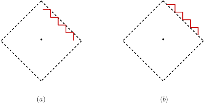
Figure 3: Covering the $n$-ball: (a) best case scenario (b) worst case scenario.

From the lower bound, we can deduce that for each ball the number of extra points covered by the robots is 5 in the best case (Fig. 3 (a)). In the worst case, the robots perform 8 units of extra amount of work (Fig. 3 (b)). So in order to cover all the points on a ball, the robots traverse a total of 13 units of extra distance. Thus, 13/5 = 2.6 is an upper bound on the amount of work per point. When robots move from the ball of radius $n$ to $n+1$, a single robot must pick up the extra point to be explored. We balance the distribution of the new work as shown in Fig. 4.

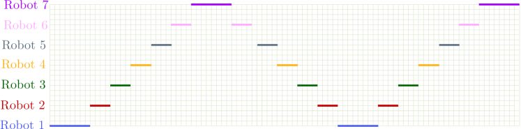
Figure 4: Allocation of additional search tasks as radius increases (x-axis). The y-axis indicates which robot is activated in that ball.

After covering the ball $n$, we have $2n^{2}+2n$ points covered, this is if we had the same amount of work for each point. The lower bound gives us $2n^{2}+5n$ amount of work to cover all the points at distance $n$. When we look at the last $4n$ points (on the $n$ ball), for each of the $4n$ points, we have $3n$ work. Thus, 7/4 amount of work per point (lower bound). From where we get the relation: $\frac{\lceil n/k\rceil(1+8/5)}{\lceil n/k\rceil(1+3/4)}=\frac{13/5}{7/4}=1.486.$ and $5\cdot 1.486=7.428.$∎

3.2 Parallel search with any number of robots

This case illustrates how the abstract search strategy for a number of robots multiple of four can readily be adapted to an arbitrary number of robots. Let $k$ be the number of robots, where $k$ is not necessarily divisible by 4.

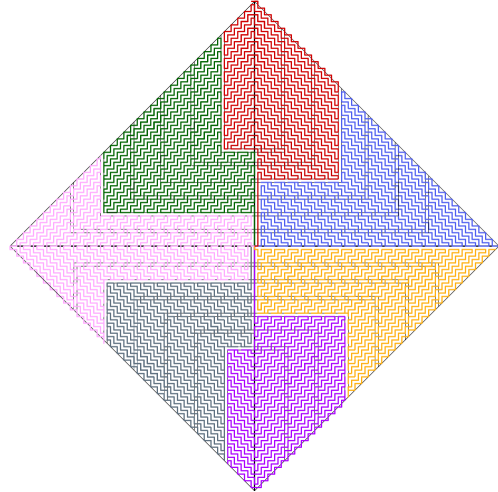
Figure 5: Parallel search with 7 robots.

We first design the strategy for $4k$ robots obtaining 4 times as many regions as robots. We then assign to every robot 4 consecutive regions as shown in Fig. 5 for the case $k=7$. Observe that now some of the regions span more than one quadrant and how the search path for each robot transitions from region to region while exploring the same ball of radius $n$ in all four regions assigned to it. Observe that from Theorems 2.2 and 3.1, it follows that this strategy searches the plane optimally as well.

Theorem 3.2

Searching in parallel with $k$ robots for a point at an unknown distance in the lattice has an asymptotic competitive ratio of at most $(2n+7.42)/k$.

4 From theory to practice

4.1 The Search Strategy

In Fig. 6, we show the search strategy with $k=4r$ robots. The snapshots are taken at search time $t=40,80,160$ and $t=260$. Since the robots traverse at unit speed, the total area explored by each robot is $t$ while the combination of all robots is $kt$.

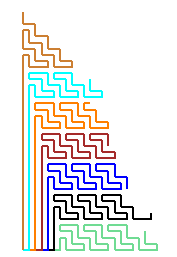
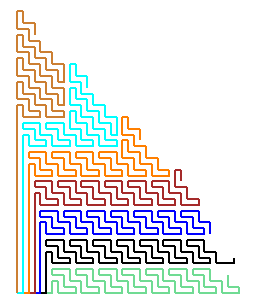
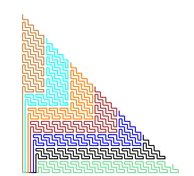
Figure 6: Parallel search with $r=7$ robots at time $t=40,80,160,240$.

While we envision the swarm of robots being usually deployed from a single vessel and as such all of them starting from the same original position, for certain searches additional resources are brought to bear as more searchers join the search-and-rescue effort. In this setting we must consider an agent or agents joining a search effort already under way.

Theorem 4.1

There exists an optimal strategy for parallel search with $k$ initial robots starting from a common origin and later adding new robots to the search.

Proof

In this case we can compute the exact time at which the additional searcher will meet up with the explored area and have the search agents switch from a $k$ robot search pattern to a $k+1$ search pattern. The net cost of this transition effort is bounded by the diameter of the $n$ ball at which the extra searcher joins, with no ill effect over the asymptotic competitive ratio. Hence, the search is asymptotically optimal. ∎

Parallel search with $k$ robots with different speeds is another case which nicely illustrates how the abstract search strategy for robots with equal speed can be readily adapted to robots of varying speeds.

Theorem 4.2

There exists an optimal strategy for parallel search with $k$ robots with different speeds.

Proof

Suppose we are given $k$ robots with varying speeds. Let the speed of the $k$ robots be $s_{1},s_{2},\ldots,s_{k}$ respectively. We can consider the speeds to be integral, subject to proper scaling and rounding. Let $s=\sum_{i=1}^{k}s_{i}$. We use the strategy for $4s$ robots and we assign for each robot respectively: $4s_{1},4s_{2},...,4s_{k}$ regions. It follows that every robot completes the exploration of its region at the same time as any other robot since the difference in area explored corresponds exactly to the difference in search speed and the search proceeds uniformly and optimally over the entire range as well. ∎

4.2 Probability of detection

In real life settings there is a substantial probability that the search agent might miss the target even after exploring the immediate vicinity of the target. Indeed, in searches on high or stormy seas often multiple passes must be made before a man overboard is located and rescued. In this case, the search vessel uses a nautical pattern resembling a clover and is known as sector search. (See [10, 12] for a robotics perspective of sector searches and other SAR techniques).

The search-and-rescue literature provides ready tables of probability of detection (POD) under various search conditions [6, 7, 8]. Fig. 7 shows the initial probability map for a typical man overboard event. Fig. 8 shows the probability of detection as a function of the width of the search area spanned. The unit search width magnitude is computed using location, time, target and search-agent specific information such as visibility, lighting conditions, size of target and height of search vessel. We consider then a setting in which a suitable POD distribution has been computed taking into account present visibility conditions and size of target (see Fig. 7). Armed with this information, a robot must then make a choice between searching an unexplored cell in the lattice or revisiting a previously explored cell.

Figure 7: Initial probability map [7].

Consider first a model in which a robot can “teleport” from any given cell to another, ignoring any costs of movement related to this switch. The greedy strategy consists of robots moving to the cell with current highest probability of containing the target. Each cell is then searched using the corresponding pattern for the number of robots deployed in the cell.

Lemma 1

Greedy is the optimal strategy for searching a probabilistic space under the teleport model.

Proof

Let $p^{j}_{i}$ be the probability of discovering the target in cell $i$ during the $j$ visit, sorted in decreasing order. We now relabel them $p_{1},p_{2},\ldots$ The expected time of discovery is $\sum_{t=1}^{\infty}p_{t}\cdot t$ which is minimized when $p_{t}$ are in decreasing order, which can be shown formally via a standard greedy technique proof. ∎

While we introduce the teleportation model as a means of understanding the complexity of the problem, observe that in real life robots could potentially be redeployed using means such as air lifting with orders of magnitude faster traveling speeds than surface searching vessels. As such, the teleportation cost would be a lower order term though never strictly zero.

In what follows we study more carefully the case where moving from one search position to another happens at the same speed as searching and hence, transit time should be accounted for in the algorithm.

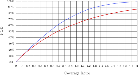
Figure 8: Average probabilities of detection (POD) over an area for visual searches using parallel sweeps (blue line: ideal search conditions, red line: normal search conditions) [7].

Observe that the probability of each cell evolves over time. It remains at its initial value so long as it is still unexplored and it becomes $(1-p)^{m}$ times its initial value after $m$ search passes, where $1-p$ is the probability of not detecting a target present in the current cell during a single search pass.

4.2.1 High Level Description of the Search Strategy.

In real life, of course, there is a cost associated with moving from a cell to another. In this case, the algorithm creates supercells of size $h\times h$ unit cells, for some value of $h$, which depends on the total number of robots available to the search effort.

The algorithm computes the combined probability of the target being found in a supercell which corresponds to the sum of the individual probabilities of the unit cells as given by the POD map.

At each time $t$, the algorithm considers the highest probability key supercell and compares it to the lowest probability key supercell being explored to determine if a robot transfer should take place. If so, it updates the probabilities of discovery accordingly. The search process continues ad infinitum or until the probability of finding the target falls below a certain threshold, in which case we consider that the object is irretrievably lost.

The process above is used to compute the number of robots gained/lost by each supercell. Once the probabilities have been rebalanced, we need to determine the source/destination pair for each robot. This is important since the distance between source and destination is dead search time, so we wish to minimize the amount of transit time. To this end, we establish a minimum-cost network flow [14] that computes the lowest total transit cost robot reassignment that satisfies the computed gains and losses.

4.2.2 Probabilistic Search Algorithm.

More formally, let $C^{t}_{1},C^{t}_{2},\ldots,C^{t}_{j}$ be the areas being explored at time $t$ by $r^{t}_{1},r^{t}_{2},\ldots,r^{t}_{j}$ robots respectively for $r_{i}\geq 0$. The combined probability of a supercell is the sum of the probabilities of the cells inside it.

These combined probabilities are then sorted in decreasing order and the algorithm dispatches robots to the highest probability supercell until the marginal value of the robots is below that of an unexplored supercell. More precisely, let $C_{i}$ and $C_{j}$ be the two supercells of highest combined probability, $p_{i}$ and $p_{j}$, respectively. The algorithm then assigns $s$ robots to supercell $C_{i}$ such that

$$p_{1}/s\geq p_{2}>p_{1}/(s+1).$$ (1)

The algorithm similarly assigns robots to $C_{j}$, $C_{m}$, and so on, updating the discovery probability per robot for each supercell. Observe that if more than one robot is assigned to $C_{j}$, the algorithm might need to increase the assignment of robots to $C_{i}$ so that Ineq. 1 is re-established.

This process continues until all $k$ robots have been allocated, and the search begins. More specifically, the algorithm maintains two priority queues. One is a max priority queue (PQ) of supercells using the combined probability per robot as key. That is, supercell $i$ appears with priority key equals to $p_{i}/(r_{i}+1)$ where $r_{i}$ is the present number of robots assigned to it by the algorithm. The other is a min PQ of supercells presently being explored with the residual probability $p_{i}/r_{i}$ of each as key.

The algorithm then compares the top element in the maxPQ with the top element in the minPQ. If the probability of the maxPQ is larger than the minPQ it adds an additional robot to the maxPQ node, and decrements its key with updated priority. Similarly, the minPQ node losses a robot and its priority is incremented due to the loss of one robot.

As the cells within a supercell are explored, the probability that the target is contained in the supercell is updated according to the probability of missing the target in an explored cell.

When the probability of the least likely supercell currently being explored falls below that of a supercell in the maxPQ we transfer a robot from the present supercell to the maxPQ supercell. The minPQ supercell gets an increased probability while the maxPQ supercell gets a decreased probability resulting from the respective decrease/increase in the number of robots in the denominator. The keys are updated accordingly in both priority queues and the algorithm continues transferring robots from minPQ supercells to maxPQ supercells. The algorithm however, does not remove the last robot from a supercell until all cells within it have been explored at least once.

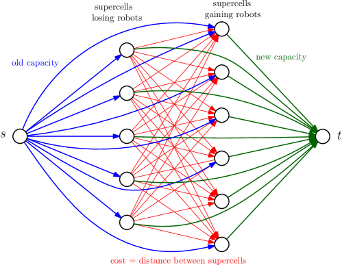
Figure 9: Optimal robot reassignment via minimum cost network flow.

Once the algorithm has computed the number of robots gained/lost by each supercell, it establishes a minimum cost network flow problem to compute the lowest total transit cost robot-reassignment schedule that satisfies the computed gains and losses.

This is modelled as a network flow in a complete bipartite graph (see Fig. 9). In this graph, nodes on the left side of the bipartite graph correspond to supercells losing robots, while nodes on the right correspond to supercells gaining robots. Every node (both losing and gaining) has an incoming arc from the source node with capacity equal to the old number of robots in the associated supercell and cost zero. Similarly, all nodes are connected to the sink with an edge of capacity exactly equal to the updated robot count of the associated supercell and cost zero as well. Lastly, the cross edges in the bipartite graph have infinite capacity and cost equal to the distance between the supercells represented by the end points.

From the construction it follows that the only way to satisfy the constraints is to reassign the robots from the losing supercell nodes to the gaining supercell nodes at minimum travel cost. This network flow problem can be solved in $O(E^{2})$ time using the algorithm of Orlin [13]. In this case $E=O(n^{2})$ and hence, in the worst case the minimum cost network flow algorithm runs in time $O(n^{4})$ where $n$ is the number of supercells.

We summarize this algorithm as the following theorem:

Theorem 4.3

The probabilistically weighted distributed scheduling strategy for the time interval $[0,t]$ can be computed in $O(t\,n^{4})$ steps, where $n$ is the size of the search grid.

4.3 Time to discovery

There are several parameters of a SAR cost. First is the total cost of the search effort as measured in vessel and personnel hours times the number of hours in the search. The second is the effectiveness of the search in terms of the probability of finding the target. Lastly, the time to discovery or speed-to-destination as time is of the essence in most search rescue scenarios. That is to say, a multiple robot search is preferable to a single agent search with the same cost and probability of detection as time to discovery is lower. Observe as well that multiple robots allow for higher coverage of the unit search width, dramatically increasing the probability of detection. The strategies presented in this paper suggest that robot swarm searches outperform traditional searches in all three of these parameters.

5 Conclusion

We present optimal strategies for robot swarm searches under both idealized and realistic considerations. The search strategies are based on a theoretical search primitive which is then enriched with realistic considerations. Interestingly, the theoretical model is resilient to these assumptions and can be readily adapted to take them into consideration. We give pseudo-code showing that the search primitives are simple and can easily be implemented with minimal computational and navigational capabilities. We then give a heuristic to account for the probability of detection map often available in real life searches. The strategies proposed have a factor of $k$ improved time to discovery as compared to a single searcher for the same total travel effort.

6 Appendix

Let $k=4r$ be the number of robots searching in parallel starting from a common origin. The following pseudo-code describes the algorithm of parallel search using $r$ robots for the first quadrant. A simple rotation applied to the code gives the search strategy for the other three quadrants, which we omit for reasons of clarity.

Algorithm 1 Strategy$(r,n)$

  Input: Let $k=4r$ the number of robots, and let $n$ be the covered distance.

  Output: parallel search strategy of $r$ robots in a quadrant.

  Robot-1($n$).

  for $i=2$ to $r-1$  do

     Middle-robots($i,\;n$).

  end for

  Robot-r($n$).

Algorithm 2 Robot-1($n$)

  Input: Let $k=4r$ the total number of robots and let $n$ be the covered distance.

  Output: The parallel search strategy of the first robot in a quadrant.

  Initialization($r$, 0);

  for $v=1$ to $n$ do

     for $j=1$ to $2(r-1)$ do

        Stairs($8(v-1)+3$, $horizontal$, $NW$).

        Stairs($8(v-1)+5$, $horizontal$, $SE$).

     end for

     for $j=1$ to $2$ do

        Stairs($4j+8(v-1)$, $horizontal$, $NW$).

        Stairs($4j+2+8(v-1)$, $vertical$, $SE$).

     end for

  end for

Algorithm 3 Initialization($x,y$)

  Input: Let $(x,y)$ be the initial starting point.

  Output: Constructs the initial pattern for a robot

  2 up.

  1 right.

  2 down.

  3 right.

Algorithm 4 Stairs($n$, $d$, $direction$)

  Input: Let $n$ be the number of steps in the stair, $d$ - the initial horizontal or vertical step and $direction$ either $NW$ for North-West or $SE$ for South-East.

  Output: The stairs in direction $direction$ starting with the first step $d$.

  if $direction=NW$ then

     1 up.

     Init-Stair($n$, $d$, $NW$).

     1 up.

  else

     1 right.

     Init-Stair($n$, $d$, $SE$).

     1 right.

  end if

Algorithm 5 Init-Stair($n$, $d$, $direction$)

  Input: Let $n$ be the number of steps in the stair, $d$ - the initial horizontal or vertical step and $direction$ either $NW$ for North-West or $SE$ for South-East.

  Output: The $n$ stairs in direction $direction$ starting with the first step $d$.

  if $n>1$  then

     if $d=horizontal$  then

        if $direction=NW$ then

           2 left.

        else

           2 right.

        end if

        Init-Stair($n-1$, $vertical$, $direction$).

     else

        if $direction=NW$ then

           2 up.

        else

           2 down.

        end if

        Init-Stair($n-1$, $horizontal$, $direction$).

     end if

  end if

Algorithm 6 Middle-robots($i,\;n$)

  Input: Let $k=4r$ the total number of robots, $i$ - the number of the current robot and let $n$ be the covered distance.

  Output: The parallel search strategy of $r-2$ (middle) robots in a quadrant.

  Initialization($r-i+1,5*(i-1)$).

  for $v=1$ to $n$  do

     for $j=1$ to $2(r-i)$  do

        Stairs($3+8(v-1)$, $horizontal$, $NW$).

        Stairs($5+8(v-1)$, $horizontal$, $SE$).

     end for

     Stairs($4+8(v-1)$, $horizontal$, $NW$).

     Stairs($6+8(v-1)$, $vertical$, $SE$).

     Stairs($8+8(v-1)$, $horizontal$, $NW$).

     for $j=1$ to 2(i-1)  do

        Stairs($7+8(v-1)$, $vertical$, $SE$).

        Stairs($9+8(v-1)$, $vertical$, $NW$).

     end for

     Stairs($10+8(v-1)$, $vertical$, $SE$).

  end for

Algorithm 7 Robot-r($n$)

  Input: Let $k=4r$ the total number of robots and let $n$ be the covered distance.

  Output: The parallel search strategy of the $r$th robot in a quadrant.

  Initialization(1, $5(r-1)$);

  Stairs($8(v-1)+4$, $horizontal$, $NW$).

  Stairs($8(v-1)+6$, $vertical$, $SE$).

  Stairs($8(v-1)+8$, $horizontal$, $NW$).

  for $j=1$ to $2(r-1)$ do

     Stairs($8(v-1)+7$, $vertical$, $SE$).

     Stairs($8(v-1)+9$, $vertical$, $NW$).

  end for

  for $v=2$ to $n$ do

     for $k=1$ to $2$ do

        Stairs($8(v-1)+4k-2$, $vertical$, $SE$).

        Stairs($8(v-1)+4k$, $horizontal$, $NW$).

     end for

     for $j=1$ to $2(r-1)$ do

        Stairs($8(v-1)+7$, $vertical$, $SE$).

        Stairs($8(v-1)+9$, $vertical$, $NW$).

     end for

  end for

References

- [1] S. Alpern and S. Gal. The Theory of Search Games and Rendezvous, Kluwer, 2002.
- [2] R. Baeza-Yates, J. Culberson and G. Rawlins. Searching in the plane, Inf. and Comp., vol. 106, (1993), pp. 234-252.
- [3] R. Baeza-Yates, R. Schott. Parallel searching in the plane, Comp. Geom.: Theory and Applications, Vol. 5, (1995), pp. 143-154.
- [4] Clear Path Robotics Inc., http://www.clearpathrobotics.com/
- [5] Canadian Coast Guard/Garde Cotiere Canadienne. Merchant ship search and rescue manual, (CANMERSAR), (1986).
- [6] IMO IAMSAR Manual. Organization and Management, vol. I, (2010).
- [7] IMO IAMSAR Manual. Mission Co-Ordination, vol. II, (2010).
- [8] IMO IAMSAR Manual. Mobile Facilities, vol. III, (2010).
- [9] B. O. Koopman, Search and screening, Report No. 56 (ATI 64 627), Operations Evaluation Group, Office of the Chief of Naval Operations, Washington, D.C., 1946.
- [10] A. López-Ortiz, On-line target searching in bounded and unbounded domains, Ph.D. thesis, University of Waterloo, 1996.
- [11] A. López-Ortiz and G. Sweet, Parallel Searching on a Lattice, Proc. of the 13th Canadian Conference on Computational Geometry (CCCG), (2001).
- [12] National Search and Rescue Secretariat/Secrétariat national Recherche et sauvetage. CANSARP, SARScene, Vol. 4, July 1994.
- [13] J.B. Orlin, A polynomial time primal network simplex algorithm for minimum cost flows, Mathematical Programming 78 (1997) pp. 109–129.
- [14] C.H. Papadimitriou and K. Steiglitz, Combinatorial Optimization: Algorithms and Complexity, Dover Publications INC, 1998.
- [15] L.D. Stone, Revisiting the SS Central America Search, International Conference on Information Fusion (FUSION) 2010, pp. 1-8.
- [16] U.S. Coast Guard Addendum to the U.S. National Search and Rescue Supplement (NSS) to the IAMSAR Manual. COMDTINST M16130.2F, January 2013.