Formation of stars and clusters over cosmological time

Abstract

The concept that stars form in the modern era began some 60 years ago with the key observation of expanding OB associations. Now we see that these associations are an intermediate scale in a cascade of hierarchical structures that begins on the ambient Jeans length close to a kiloparsec in size and continues down to the interiors of clusters, perhaps even to binary and multiple stellar systems. The origin of this structure lies with the dynamical nature of cloud and star formation, driven by supersonic turbulence and interstellar gravity. Dynamical star formation is also relatively fast compared to the timescale for cosmic accretion, and in this limit of rapid gas consumption, the star formation rate essentially keeps up with the accretion rate, whatever that rate is, leading to a sequence of near-equilibrium states during galaxy formation and evolution. In these states, most of the large-scale and statistical properties of galaxies and of star formation inside them depend on the rate of cosmic accretion, which is a function of galaxy mass and epoch. This simplification of star formation on a cosmic scale allows successful simulations and modeling even when the details of star formation on the scale of molecular clouds is unclear. Dynamical star formation also helps to explain the formation of bound clusters, which require a local efficiency that exceeds the average by more than an order of magnitude. Efficiency increases with density in a hierarchically structured gas. Cluster formation should vary with environment as the relative degree of cloud self-binding varies, and this depends mostly on the ratio of the interstellar velocity dispersion to the galaxy rotation speed. As this ratio increases, galaxies become more clumpy, thicker, and have more tightly bound star-forming regions. The formation of old globular clusters is understood in this context, with the metal-rich and metal-poor globulars forming in high-mass and low-mass galaxies, respectively, because of the galactic mass-metallicity relation. This relation is a result of the accretion equilibrium. Metal-rich globulars remain in the disks and bulge regions where they formed, while metal-poor globulars get captured as parts of satellite galaxies and end up in today’s spiral galaxy halos. Blue globulars in the disk could have formed very early when the whole Milky Way had a low mass.

1 Celebrating the Beginnings: 60 and 64 years ago

A good place to begin this story is with the publications by Viktor Ambartsumian in 1949 and 1950, and then again in the Western literature in 1954, of his discovery that luminous stars are in loose associations that expand over time. This was the beginning of the modern era of star-formation research. The only explanation for the systematic motion was that the associations are young, with expansion ages of several million years, and therefore that the stars themselves are young. Before this, astronomers could not really tell if star formation was still going on in the present-day universe. The age of the solar system, galactic stars, and the Hubble time were all thought to be about 3 Gyr (see 1935 Science Volume 82). Blaauw (1952) quickly confirmed Ambartsumian’s discovery. Prior speculation about the mechanisms and locations of star formation (Bok, 1936; Edgeworth, 1946; Whipple, 1946; Spitzer, 1949), whether it took place in the early universe or more recently (as suggested to Spitzer by the high luminosities of supergiant stars), suddenly fell into place.

A flurry of activity followed. In 1952 Herbig speculated that the variable stars he had been studying in nebulae could actually be young and not just interacting with nearby gas. Öpik (1953) proposed that stellar associations expanded because of supernova-induced star formation, and Zwicky (1953) proposed that the expansion came from cluster unbinding as the gas left. Morgan et al. (1953) discovered spiral arms in the Milky Way from the positions of OB associations. Hoyle (1953) proposed that collapsing clouds would fragment, making clusters. Soon after, Salpeter (1955) determined the distribution function of stellar masses at intermediate mass in the solar neighborhood. Also at about this time, Ewen & Purcell (1951) and Muller & Oort (1951) discovered the 21 cm emission line of hydrogen, after which Lilley (1955) determined the gas-to-dust ratio, and Bok (1955) found that dark clouds had too little HI for their dust, suggesting that the gas is molecular.

It is interesting to note that a possible impediment to early recognition that the interstellar medium is gravitationally unstable to collapse into clouds and stars was the wrong gas-to-dust ratio; the interstellar gas mass was thought to be too low by a factor of $\sim 10$ (see Spitzer, 1941, page 243). This was before interstellar HI was detected, and, although heavy elements like sodium and calcium were observed in interstellar absorption lines, it was also before the extent of their depletion onto grains was known. Oort (1932) showed from vertical gravity that the non-stellar mass amounted to an average density of about 1 atom cm^-3, but the form of this matter was not known (he included meteorites in his possible list of mass contributors). Thus Spitzer (1941) and Whipple (1946) tried to make stars by the convergence of radiation pressure on mutually shielding dust particles, which had a 1/2 Gyr timescale in the ambient medium. The idea that a medium with an average density of $\sim 1$ atom cm^-3 could be gravitationally unstable on an enormous scale, forming kiloparsec-size cloud complexes with a cascade to smaller scales forced by supersonic turbulence, had to wait for a more general understanding of spiral structure and large-scale disk dynamics, and for extensive observations of correlated gas structures and motions. (For a review of the contributions by Lyman Spitzer Jr. to the early developments of star formation theory, see Elmegreen, 2009).

A personal milestone was the IAU Symposium 76 on “Star Formation,” held in Geneva Switzerland in 1976. This marked the year of my first publication on this topic. It was also a good place for a honeymoon. In the context of the present talk, the conference summary by Donald Lynden-Bell (1977) was noteworthy. There he said: “There are three great areas of astronomy to which a theory of star formation is vital,” and the first area listed was “The formation and evolution of galaxies.” For this he described a complicated hypothetical star formation rate ${\cal R}$ that is a function of many environmental variables but then said “However, if we knew the true functional form of ${\cal R}$ and offered it to a galaxy builder he would probably tell us ‘Oh, go jump in the lake, that’s far too complicated’. Thus galaxy builders need oversimplified average laws like Schmidt’s suggestion ${\cal R}=C\rho^{2}$.” After much research since then by a large community on star formation triggering in pillars, shells, spiral arms, and supersonically compressed turbulent clouds, we have come back to Lynden-Bell’s suggestion.

2 The Oversimplified Average Law

“Oversimplified average laws” like the Schmidt law, or, in today’s terms, the Kennicutt-Schmidt law, have indeed become the preferred form for galaxy builders. In fact, the star formation law can be even simpler, i.e., linearly proportional to total galactic gas mass, and even then most of the statistical properties of galaxies can be derived without regard to detailed processes on stellar scales. These properties include the distribution functions of stellar, gaseous, and metal masses over cosmic time, along with the star formation rates. The reason for this simplification is that the star formation timescale in terms of the time to use up the available gas is generally shorter than the timescale for cosmic evolution. Then star formation keeps up with the accretion rate and all of these large-scale distribution functions depend primarily on the properties of cosmic accretion (Larson, 1972; Edmunds, 1990; Davé et al., 2012; Lilly et al., 2013; Dekel et al., 2013; Peng & Maiolino, 2014).

Following Dekel et al. (2013), the baryonic accretion rate through the galaxy virial radius at redshift $z$ is

$${{dM_{\rm acc}}\over{dt}}=30f_{b}M_{\rm halo,0,12}e^{-0.79z}(1+z)^{2.5}\;M_{\odot}\;{\rm yr}^{-1},$$ (1)

where $M_{\rm halo,0,12}$ is the halo mass today in units of $10^{12}\;M_{\odot}$ (equal to about 2 for the Milky Way), and the baryonic fraction is $f_{b}=0.16$. The accretion rate to the disk could be about the same as the rate through the virial radius when the halo mass is equal to or less than $10^{12}\;M_{\odot}$, because then accretion mostly penetrates the halo in a cold flow (Kereš et al., 2005; Dekel & Birnboim, 2006). For a review of accretion and star formation, see Sánchez Almeida et al. (2014).

The star formation rate in these simple models is

$${\rm SFR}=M_{\rm gas}/\tau$$ (2)

for gas consumption time $\tau$ that may depend on stellar or halo mass and redshift. Gas is also lost to the halo in a wind at the rate

$${{dM_{\rm gas}}\over{dt}}=-w\times{\rm SFR}$$ (3)

where $w$ is the mass loading factor for winds ($w\sim 1$ in Peng & Maiolino, 2014); $w$ may also depend on galaxy mass and redshift (Zahid et al., 2014). If stars return a fraction $R$ ($\sim 0.4$; Peng & Maiolino, 2014) of their mass to the interstellar medium, then the interstellar mass varies with time as

$${{dM_{\rm gas}}\over{dt}}={{dM_{\rm acc}}\over{dt}}-(1-R+w)M_{\rm gas}/\tau.$$ (4)

If $\tau$ is small compared to timescales for changes in the accretion rate, then there is a steady state where $dM_{\rm gas}/dt\sim 0$ and

$${\rm SFR}\sim\left(1\over{1-R+w}\right){{dM_{\rm acc}}\over{dt}}.$$ (5)

Dekel et al. (2013) show that these equations compare well to numerical simulations. They also derive the consumption time $\tau$ to be about $0.17t_{\rm H}$ for instantaneous Hubble time $t_{\rm H}$. This time relation comes from the ratio of the virial radius to the virial speed, which depends on $t_{\rm H}$, combined with the ratio of the disk radius to the virial radius, which comes from the halo spin parameter, plus the similarity between the free fall time at the average gas density and the disk dynamical time, and the efficiency of star formation per unit free fall time. The point is that $\tau$ is smaller at earlier times and always small enough to keep the galaxy in a quasi-equilibrium state, even when the galaxy is young.

Equation (2) comes from a more fundamental relation

$${\rm SFR/Volume}=\epsilon_{\rm ff}\rho/\tau_{\rm ff}$$ (6)

where $t_{\rm ff}$ is the free fall time and $\epsilon_{\rm ff}$ is the fraction of the gas mass that turns into stars in a free fall time. Generally $\epsilon_{\rm ff}$ is small, several per cent, for densities close to the average interstellar density (Krumholz & Tan, 2007). Krumholz et al. (2012) show that all regions of star formation, ranging from individual molecular clouds to normal galaxies to starburst galaxies to high-redshift galaxies, satisfy this relation if the free fall time is taken to be the minimum of two values, the value for giant molecular clouds, which have much higher densities than the average ISM in normal disks, and the value for the ambient medium, with the additional conditions that the gas pressure is determined by the weight of the mass column density and the Toomre instability parameter is constant and of order unity.

3 Why is $\epsilon\sim 0.01$?

The low value of $\epsilon_{\rm ff}\sim 0.01$ suggests a broad spectrum of possibilities, ranging from molecular clouds and other interstellar gas that is prevented from collapsing for several tens of free fall times, to the presence of only a small fraction of the gas in a form that can collapse into a star, with a rapid collapse rate for this small fraction. The observation of bound star clusters that form locally in only several free fall times (Getman et al., 2014) suggests that $\epsilon_{\rm ff}$ is actually high in dense regions, because a high total efficiency is necessary to keep the stars bound to the cluster after the gas leaves (Parmentier & Fritze, 2009). In this case $\epsilon_{\rm ff}$ should be an increasing function of density. However, such an increase is inconsistent with the expected speed-up of collapse at high density: $\epsilon_{\rm ff}M/\tau_{\rm ff}$ in a region of total mass $M$ should give the same star formation rate whether it is measured at high density or low density. Because $\tau_{\rm ff}\propto\rho^{1/2}$, $\epsilon_{\rm ff}$ should scale as $\rho^{-1/2}$ to keep $\epsilon_{\rm ff}M/\tau_{\rm ff}$ constant if $M$ is constant.

A solution to this problem (Elmegreen, 2002) is that only a low fraction of the total mass $M$ can be at a high density, collapsing rapidly on its local dynamical time, while a much larger fraction of $M$ is at a low density, collapsing slowly or unable to collapse at all on its own dynamical time. The collapsing fraction has to decrease with increasing average density. Thus $\epsilon_{\rm ff}$ should be viewed as including a term equal to the fraction of the gas at a density greater than $\rho$ (Elmegreen, 2008). Then the star formation rate is independent of the scale of measurement because

$$\epsilon_{\rm ff}(\rho)\rho^{1/2}f_{\rm M}(\rho)=\epsilon_{\rm ff}(\rho_{0})\rho_{0}^{1/2}f_{\rm M}(\rho_{0})$$ (7)

for either some normalization at an average density $\rho_{0}$, or, what is more physically motivated, a normalization at a some high density $\rho_{0}$ where the local efficiency has its maximum possible value close to unity. Here $f_{\rm M}(\rho)$ is the mass fraction at density larger than $\rho$. Depending on the details of collapse and cloud structure, we could alternatively write the above equation as

$$\epsilon_{\rm ff}(\rho)\int_{\rho}\rho^{1/2}f^{\prime}_{\rm M}(\rho)d\rho=\epsilon_{\rm ff}(\rho_{0})\rho_{0}^{1/2}f_{\rm M}(\rho_{0})$$ (8)

where $f^{\prime}$ is the differential form of $f$, namely the fraction of the gas between density $\rho$ and $\rho+d\rho$. As a result of these considerations, the local efficiency increases with $\rho$ as

$$\epsilon_{\rm ff}(\rho)=\epsilon_{\rm ff}(\rho_{0})\left({{\rho_{0}}\over{\rho}}\right)^{1/2}{{f_{\rm M}(\rho_{0})}\over{f_{\rm M}(\rho)}}.$$ (9)

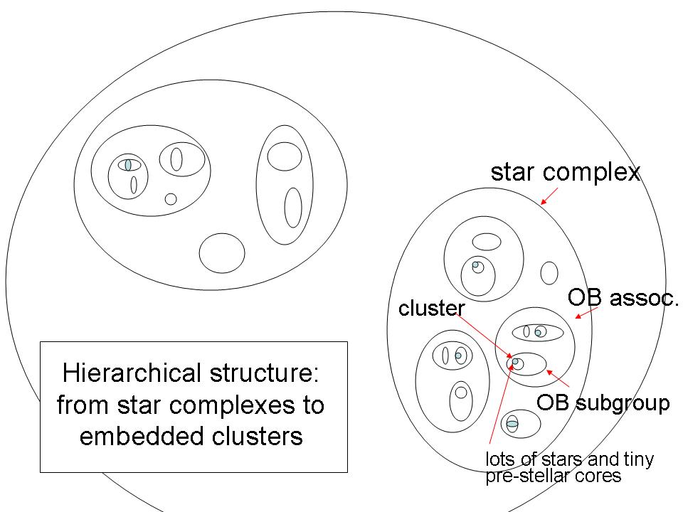
Figure 1: Schematic showing hierarchical structure with smaller and younger star formation regions nested inside larger and older star forming regions. As we zero in on the densest regions, the low-density inter-region gas gets left behind and the average density increases. Also increasing at the same time is the fraction of the gas at this high density that is at even higher density. If the efficiency of star formation in some region is the mass fraction of the densest sub-clumps (where stars form), then this mass fraction increases with average density simply because of the hierarchical structure. The efficiency therefore increases with average density.

The mass fraction $f_{M}(\rho)$ is most likely determined by turbulent fragmentation (Elmegreen, 2002, 2008), which makes this function a log-normal in weakly self-gravitating regions or a log-normal with a power-law tail in strongly self-gravitating regions (Klessen, 2000; Vázquez-Semadeni et al, 2008; Kritsuk et al., 2011; Elmegreen, 2011). Turbulent fragmentation partitions a cloud hierarchically so that dense regions are inside and to the side of lower-density regions (Burkhart et al., 2013). With hierarchical structure, the fraction of the mass in the highest density regions increases as the average density increases (Figure 1). If we consider that the formation of a bound cluster requires a certain minimum local efficiency, like $\sim 10-20$%, depending on the timescale for gas clearing (it has to be 50% in the immediate neighborhood of the stars for rapid clearing), then this minimum local efficiency corresponds to a minimum average local density in comparison to the fiducial density $\rho_{0}$ (Elmegreen, 2008, 2011). Thus star formation at low average density, as in star complexes (Efremov, 1995) or OB associations, has a low efficiency, several percent, and leaves the stars expanding, as found by Ambartsumian 64 years ago. Star formation at high average density, inside molecular cloud cores, for example, has a high efficiency, 10% or more, often leaving a bound cluster. At even higher density, where individual or multiple stellar systems form, the efficiency can approach 50% or more. There is no characteristic length or mass scale for star formation (aside from the lower mass limit to the power law in the initial stellar mass function). Stellar groupings form with a wide range of densities, following the log-normal distribution (Bressert et al., 2010).

This simplified view of bound cluster formation glosses over many details, of course, but it has predictive value and it coincides qualitatively with the current picture of star formation in a turbulent medium. One prediction of it is that the density at which star formation becomes highly efficient, perhaps viewed as a critical density for star formation or a density at which self-gravity becomes stronger than other forces, should increase in regions with higher Mach number and/or higher average density. The critical density should be viewed as relative to the average rather than as absolute. This prediction comes from the efficiency function $\epsilon(\rho)$, which, for a log-normal density pdf and mass function $f_{\rm M}(\rho)$, reaches a certain high value when the density exceeds a certain multiple of the average. There is no absolute scale in this argument. Moreover, the ratio of the density at high efficiency to the average density increases with both Mach number (Elmegreen, 2008) and central concentration of the cloud (Elmegreen, 2011). Higher pressures should therefore correspond to higher threshold densities, a higher fraction of star formation in bound clusters, and denser clusters. Applications of this scaling to the central molecular zone of galaxies were made by Kruijssen et al. (2014), who explained the modest star formation rate there (considering the $\times 100$ density compared to the disk) as a result of a higher threshold density.

Another application is to clumpy galaxies, such as high redshift clumpy galaxies and local dwarf irregulars. As discussed more in Sections 6 and 7 below, clumpy galaxies have high ratios of velocity dispersion to rotation speed. In this case the relative binding energy of the star-forming regions is high too. Such high binding energy corresponds to more strongly concentrated clouds and a higher mass fraction forming stars at high efficiency, according to the discussion above. Thus we predict a higher fraction of star formation in bound clusters, and possibly denser clusters, in clumpy galaxies than in smooth-disk galaxies.

Also important in the determination of $\epsilon$ is the geometry of the star-forming gas at high density, which tends to be filamentary (e.g. Hacar et al., 2013; Palmeirim et al., 2013). Filamentary gas drains down to cores on a timescale equal to about the dynamical time, $(G\rho)^{-1/2}$, for local filament density $\rho$, multiplied the ratio of the length to width of the filament. This extra multiplicative factor is the result of gravity being an isotropic central force with a dynamical time proportional to the inverse square root of the average density inside an enclosing sphere, rather than the inverse square root of the local density inside sub-regions of that sphere. Thus there is a slowness to filamentary star formation compared to spherical star formation at the same local (peak) density. This means that the accreting core can sustain prestellar growth for many local dynamical times as the attached filament or filaments drain into it. Still the process is dynamical, that is, without equilibrium from feedback or delays from magnetic diffusion. It is just that the timing has a contribution from the geometry in addition to the local peak density.

4 Starbursts are Thick

Krumholz et al. (2012) model equation (6) in a way that allows them to convert from a volume density $\rho$ to a surface density $\Sigma$, for comparison with observations. To do this they make two reasonable assumptions, that the value of Toomre $Q=\kappa\sigma/\left(\pi G\Sigma\right)$ is about constant, as determined by gravitational instability feedback regulating the velocity dispersion $\sigma$ ($\kappa$ is the epicyclic frequency), and the gas pressure is determined by hydrostatic equilibrium, $\rho\sigma^{2}\sim 0.5\pi G\Sigma^{2}$. The first relation says that $\sigma\propto\Sigma$ for a given $\kappa$ and then the second says that $\rho=$ constant at that $\kappa$. This means that the midplane density is about the same in all galaxy disks of the same size and rotation rate, regardless of whether the galaxy has low or high surface brightness from star formation.

The projected star formation rate in this interpretation is $\epsilon_{\rm ff}\Sigma/t_{\rm ff}$, and so it varies only as $\Sigma$ varies for a given midplane density (i.e., fixed $t_{\rm ff}$), and $\Sigma\propto\sigma$, the velocity dispersion. Thus higher star formation rate densities correspond to higher velocity dispersions. Considering also that the galaxy thickness varies as $H\sim\sigma^{2}/\left(\pi G\Sigma\right)$ for a one-component disk, it follows that $H\propto\sigma\propto\Sigma$. Thus galaxies with a high surface brightness of star formation are thicker on the line of sight, and have a higher gas velocity dispersion, than galaxies with a low surface brightness from star formation, all else being equal. Starburst galaxies have more layers of fixed density on the line-of-sight than low-surface brightness galaxies of the same size and rotation rate. A starburst merger of a given size, like the Antennae galaxies, is thicker than an isolated galaxy (and has a larger velocity dispersion). Large HI velocity dispersions in interacting galaxies were measured long ago (Elmegreen et al., 1993) and have been modeled by computer simulations (Powell et al., 2013).

5 LEGUS

A recent HST survey of nearby galaxies in the ultraviolet, LEGUS (PI: Calzetti, 2014, in preparation) has been analyzed to determine the characteristics of hierarchical structure in star-forming regions (Elmegreen et al., 2014). There were 12 galaxies in the analysis covering a range of late Hubble types and star formation rates, including NGC 1705 and NGC 5253, which contain super star clusters. The analysis consisted of blurring the images in successively increasing sizes and counting the number of regions in each blurred image. A log-log plot of this number versus the blur scale typically gives a power law, and the slope of this power law is the projected fractal dimension.

The study indicated that the fractal dimension of a whole galaxy is higher, more like 2 than 1, in the most actively star-forming galaxies (including NGC 1705, NGC 5253, and UGC 695) and that individual regions in all of the galaxies also have high dimensions ($\sim 2$). Inactive galaxies have low overall dimensions ($\sim 1-1.5$) although their individual regions have high dimensions. This means that the basic building block for star formation is a bright patch with a high dimension, and that the most active galaxies are composed of only one or two of these patches, which essentially cover a high fraction of the disk. The less active galaxies, including some with spiral arms, typically have their star-forming regions spread out, and this gives them a lower overall fractal dimension. A high fractal dimension, $\sim 2$, corresponds to a region that is filled with emission in projection; there are relatively few empty lines of sight.

6 Clumpy Galaxies and Super Star Clusters

The number of giant star-forming regions, or star complexes, in a galaxy is an important discriminant of star formation activity. Each region typically has a size and mass comparable to the Jean length and mass at the average turbulent speed and average density of the interstellar medium. The Jeans length is essentially $\sigma/\left(G\rho\right)^{1/2}$. The galaxy size, on the other hand, scales with the rotation speed $V_{\rm circ}$ instead of the velocity dispersion, and may be written approximately as $V_{\rm circ}/\left(G\rho\right)^{1/2}$. The number of Jeans lengths in a galaxy of a given average density is therefore $(V_{\rm circ}/\sigma)^{2}$. This number is small when the gaseous velocity dispersion is a high fraction of the rotation speed. This is the case for local dwarf Irregulars and BCDs, which have about the same $\sigma$ as local spirals but lower $V_{\rm circ}$, and also for high redshift clumpy galaxies, which have about the same $V_{\rm circ}$ as local spirals but much higher $\sigma$ (Förster Schreiber et al., 2009).

The disk thickness and turbulent Jeans length are nearly the same, $\sigma^{2}/\left(\pi G\Sigma\right)$, so galaxies with high $\sigma/V_{\rm circ}$ have relatively thick disks (relative to their diameters). This is the case for local dwarf irregulars and clumpy high-redshift disks. In the case of the clumpy high-z disks, the relative thickness is presumably what produced the old thick disks in today’s galaxies (Bournaud et al., 2009). Considering the results of the previous paragraph, the relative disk thickness scales inversely with the number of giant star complexes.

7 Super Star Clusters

Now we come to the formation of super star clusters. How can some small galaxies like NGC 1705 produce a $10^{6}\;M_{\odot}$ bound cluster when large galaxies like the Milky Way only produce clusters up to $\sim 10^{5}\;M_{\odot}$? (Some local spiral galaxies have more massive clusters, Larsen & Richtler, 1999, but the Milky Way apparently does not.). The answer again seems to come down to the number of star complexes. The ratio of the gravitational binding energy in a Jeans mass cloud complex to the background energy density from the galaxy (in the form of tidal forces, shear, rotation, etc.) also involves only the ratio of $\sigma^{2}$ to $V_{\rm circ}^{2}$ (in the present approximation where background stars are ignored). This ratio of binding energy scales inversely with the number of star complexes.

It follows that morphologically clumpy galaxies produce thicker disks and have more strongly bound star-forming regions than smooth galaxies. The thicker disks (for the same galaxy size) correspond to higher star formation rates (see previous section), and the tighter self-binding reasonably transforms to a higher fraction of star formation in the form of bound clusters (Elmegreen, 2011). Greater self-binding should also correspond to a more massive cluster at the upper end of the cluster mass range, and possibly denser clusters of all mass. This shift toward a more massive largest cluster corresponds to the formation of a super star cluster at the upper end of a power law distribution of cluster masses. The power law need not change as $\sigma/V_{\rm circ}$ increases, because that is determined by turbulent and gravitational fragmentation, with some contribution from sub-cluster coalescence, which are all scale-free processes.

We can now see where the old globular clusters might have come from. The metal-rich globular clusters, which tend to coincide with the disks and bulges of today’s galaxies, were presumably made in the giant clumps of high-redshift clumpy galaxies (Kravtsov & Gnedin, 2005; Shapiro et al., 2010), which were also massive enough to hold on to their winds and metals, and thereby achieve a high metallicity. These clumpy galaxies are the predecessors of today’s giant spirals. The metal-poor globular clusters, which tend to coincide with the halos of today’s galaxies, presumably came from high redshift dwarf galaxies (Elmegreen et al., 2012), which should also have been clumpy, like today’s dwarfs, but because of their inability to contain their star-formation winds, lost the metal-enriched material that stellar evolution generated. Here we are using the galaxy mass dependence of the wind mass loading factor, $w$, discussed in section 2, to explain the mass-metallicity relationship in galaxies (Mannucci et al., 2009; Lilly et al., 2013). Metal-poor globulars associated with disk populations could have originated in-situ (Brodie et al., 2014) when the disk had a much lower mass and metallicity than today.

8 Summary

Lynden-Bell’s wish of an “oversimplified average law like Schmidt’s suggestion” came true. The law is essentially SFR$\sim\epsilon\rho/t_{\rm ff}$ or SFR$\sim M_{\rm gas}/\tau$ for $\tau\sim 0.17t_{\rm H}$ with instantaneous Hubble time $t_{\rm H}$. Because the gas depletion time $\tau$ is relatively short compared to the accretion time, whole galaxies can be in approximate equilibrium with the star formation rate equal to the cosmic accretion rate and the metallicity approximately constant, increasing only as the galaxy mass increases.

Locally, star formation is more dynamic than this, acting on a timescale of several crossing times for each region and with an efficiency that is low at the average density but increases with density, considering the hierarchical distribution of mass and density during turbulent fragmentation. This increasing efficiency explains how bound clusters can form at high density when the average efficiency is low at low density. The dependence of the efficiency on the shape of the density distribution function may also explain how the clustering fraction in star formation varies with environment, including an expected increase with $\sigma/V_{\rm rot}$ from more tightly bound clouds.

Galaxies go through a sequence of equilibrium states while star-forming regions inside galaxies change, move, and disrupt on dynamical times. The difference is that galaxies have inert dark matter halos which hold the star formation in place, while star-forming regions have nothing to hold them down but disrupt by internal processes soon after they form. Both systems accrete gas on dynamical timescales and return a high fraction of this gas to the surrounding medium, but for galaxies, the returned gas falls back into the dark matter potential, while for star formation, it moves to the side and falls into another potential when the next cloud forms.

References

- Ambartsumian (1949) Ambartsumian, V.A. 1949, AJ, USSR, 26, 3
- Ambartsumian (1950) Ambartsumian, V.A. 1950, Izv. Ak. Nauk, USSR Phys. Ser. XIV, 15
- Ambartsumian (1954) Ambartsumian, V. A. 1954, Les Processus Nucléaires dans les Astres, Communications présentées au cinquième Colloque International d’Astrophysique tenu à Liège, p. 293
- Blaauw (1952) Blaauw, A. 1952, BAN, 11, 405
- Bok (1936) Bok, B.J. 1936, Obs, 59, 76
- Bok (1955) Bok, B.J. 1955, AJ, 60, 146
- Bournaud et al. (2009) Bournaud, F., Elmegreen, B. G., & Martig, M. 2009, ApJ, 707, L1
- Bressert et al. (2010) Bressert, E., Bastian, N., Gutermuth, R., et al. 2010, MNRAS, 409, L54
- Brodie et al. (2014) Brodie, J.P., Romanowsky, A.J., Strader, J. et al. 2014, arXiv.1405.2079
- Burkhart et al. (2013) Burkhart, B., Lazarian, A., Goodman, A., Rosolowsky, E. 2013, ApJ, 770, 141
- Davé et al. (2012) Davé, R., Finlator, K., & Oppenheimer, B. D. 2012, MNRAS, 421, 98
- Dekel & Birnboim (2006) Dekel, A. & Birnboim, Y. 2006, MNRAS, 368, 2
- Dekel et al. (2013) Dekel, A., Zolotov, A., Tweed, D., et al. 2013, MNRAS, 435, 999
- Edgeworth (1946) Edgeworth, K. E. 1946, MNRAS, 106, 470
- Edmunds (1990) Edmunds, M. G. 1990, MNRAS, 246, 678
- Efremov (1995) Efremov, Y.N. 1995, AJ, 110, 2757
- Elmegreen et al. (1993) Elmegreen, B.G., Kaufman, M. & Thomasson, M. 1993, ApJ, 412, 90
- Elmegreen (2002) Elmegreen, B.G. 2002, ApJ, 577, 206
- Elmegreen (2008) Elmegreen, B.G. 2008, ApJ, 672, 1006
- Elmegreen (2009) Elmegreen, B.G. 2009 in Reviews in Modern Astronomy, Formation and Evolution of Cosmic Structures, Vol. 21, Wiley-VCH, p. 157-181
- Elmegreen (2011) Elmegreen, B.G. 2011, ApJ, 731, 61
- Elmegreen et al. (2012) Elmegreen, B.G., Malhotra, S., & Rhoads, J. 2012, ApJ, 757, 9
- Elmegreen et al. (2014) Elmegreen, D.M., Elmegreen, B.G., Adamo, A. et al. 2014, ApJ, 787, L15
- Ewen & Purcell (1951) Ewen, H. I., & Purcell, E. M. 1951, Nature, 168, 356
- Förster Schreiber et al. (2009) Förster Schreiber, N. M., Genzel, R., Bouché, N. et al. 2009, ApJ, 706, 1364
- Getman et al. (2014) Getman, K.V., Feigelson, E.D., Kuhn, M. A. et al. 2014, arXiv1403.2741
- Hacar et al. (2013) Hacar, A., Tafalla, M., Kauffmann, J., Kovács, A. 2013, A&A, 554A, 55
- Herbig (1952) Herbig, G.H. 1952, JRASC, 46, 222
- Hoyle (1953) Hoyle, F. 1953, ApJ, 118, 513
- Kereš et al. (2005) Kereš, D., Katz, N., Weinberg, D. H., & Dav’e, R. 2005, MNRAS, 363, 2
- Klessen (2000) Klessen, R. S. 2000, ApJ, 535, 869
- Kravtsov & Gnedin (2005) Kravtsov, A. V., & Gnedin, O. Y. 2005, ApJ, 623, 650
- Kritsuk et al. (2011) Kritsuk, A. G., Norman, M. L., & Wagner, R. 2011, ApJ, 727, L20
- Kruijssen et al. (2014) Kruijssen, J.M.D., Longmore, S.N., Elmegreen, B.G., et al. 2014, MNRAS, 440, 3370
- Krumholz & Tan (2007) Krumholz, M.R., Tan, J.C. 2007, ApJ, 654, 304
- Krumholz et al. (2012) Krumholz, M.R., Dekel, A., & McKee, C.F. 2012, ApJ, 745, 69
- Larsen & Richtler (1999) Larsen, S.S. & Richtler, T. 1999, A&A, 345, 59
- Larson (1972) Larson, R. B. 1972, Nature Physical Science, 236, 7
- Lilley (1955) Lilley, A. E. 1955, ApJ, 121, 559
- Lilly et al. (2013) Lilly, S. J., Carollo, C. M., Pipino, A., Renzini, A., & Peng, Y. 2013, ApJ, 772, 119
- Lynden-Bell (1977) Lynden-Bell, D. 1977, IAUS 75, 75, 291
- Mannucci et al. (2009) Mannucci F. et al., 2009, MNRAS, 398, 1915
- Morgan et al. (1953) Morgan, W. W., Whitford, A. E., & Code, A. D. 1953, ApJ, 118, 318
- Muller & Oort (1951) Muller, C. A., & Oort, J. H. 1951, Nature, 168, 357
- Oort (1932) Oort, J.H. 1932, BAN, 6, 249
- Öpik (1953) Öpik, E. J., 1953, IrAJ, 2, 219
- Palmeirim et al. (2013) Palmeirim, P., André, Ph., Kirk, J., et al. 2013, A&A, 550A, 38
- Parmentier & Fritze (2009) Parmentier, G., & Fritze, U. 2009, ApJ, 690, 1112
- Peng & Maiolino (2014) Peng, Y.-J. & Maiolino, R. 2014, MNRAS, 438, 262
- Powell et al. (2013) Powell, L.C., Bournaud, F., Chapon, D., Teyssier, R. 2013, MNRAS, 434, 1028
- Salpeter (1955) Salpeter, E.E. 1955, ApJ, 121, 161
- Sánchez Almeida et al. (2014) Sánchez Almeida, J., Elmegreen, B.G., Muñoz-Tuñón, C. & Elmegreen, D.M. 2014, A&AR, in press
- Shapiro et al. (2010) Shapiro, K.L., Genzel, R., & Förster Schreiber, N.M. 2010, MNRAS, 403, L36
- Spitzer (1941) Spitzer, L., Jr. 1941, ApJ, 94, 232
- Spitzer (1949) Spitzer, L. Jr. 1949, Astronomical Society of the Pacific Leaflets, 5, 336
- Vázquez-Semadeni et al (2008) Vázquez-Semadeni E., González, R.F., Ballesteros-Paredes, J., Gazol, A., & Kim, J. 2008, MNRAS, 390, 769
- Whipple (1946) Whipple, F. 1946, ApJ, 104, 1
- Zahid et al. (2014) Zahid, H.J., Torrey, P., Vogelsberger, M., Hernquist, L., Kewley, L., Davé, R. 2014, Ap&SS, 349, 873
- Zwicky (1953) Zwicky, F. 1953, PASP, 65, 205