Abstract: Kopparty and Wang studied in [3] the relation between the roots of a univariate polynomial over ${\mathbb{F}}_{q}$ and the zero-nonzero pattern of its coefficients. We generalize their results to polynomials in more variables.

1 Introduction

In [3] Kopparty and Wang considered the zero-nonzero pattern of a univariate polynomial $P(X)$ over ${\mathbb{F}}_{q}$ and its relation to the number of roots in ${\mathbb{F}}_{q}^{\ast}$. Their main theorem [3, Th. 1] states that a polynomial with many zeros cannot have long sequences of consecutive coefficients all being equal to zero. Then in [3, Th. 2] they gave necessary and sufficient conditions for a product of pairwise different linear factors to have sequences of zero coefficients of maximal possible length for any polynomial with prescribed number of roots. In this note we generalize the abovementioned results to polynomials in more variables.
In Section 2 we start by recalling the results by Kopparty and Wang. In Section 3 we then present and prove the generalizations.

2 Univariate polynomials

The main theorem in [3] is their Theorem 1 which we present in a slightly stronger version.

Theorem 1

Let $P(X)\in{\mathbb{F}}_{q}[X]$ be a nonzero polynomial of degree at most $q-2$, say $P(X)=\sum_{i=0}^{q-2}b_{i}X^{i}$. Let $m$ be the number of $x\in{\mathbb{F}}_{q}^{\ast}$ with $P(x)\neq 0$. Then there does not exist any $k\in\{0,\ldots,q-2\}$ where all the $m$ coefficients $b_{k}$, $b_{k+1{\mbox{ mod }}(q-1)},\ldots,b_{k+m-1{\mbox{ mod }}(q-1)}$ are zero.

The modification made in Theorem 1 is that we consider $k\in\{0,\ldots,q-2\}$ rather than just $k\in\{0,\ldots,q-1-m\}$. The proof in [3] is easily modified to cover this more general situation. Alternatively, one can deduce it by writing $P(X)=X^{s}Q(X)$ with $s$ maximal and then applying [3, Th. 1] to $Q(X)$.

Obviously, if we consider a product of $q-1-m$ pairwise different linear factors $X-x$ with $x\neq 0$, this polynomial has exactly $m$ non-roots in ${\mathbb{F}}_{q}^{\ast}$ and we have $b_{q-m}=\cdots=b_{q-2}=0$ which is a sequence of $m-1$ consecutive zero coefficients modulo $q-1$. The below theorem, corresponding to [3, Th. 2], gives sufficient and necessary conditions for a sub-sequence of $m-1$ consecutive zeros among $b_{0},\ldots,b_{q-m-2}$ to exist.

Theorem 2

Let $S$ be a subset of ${\mathbb{F}}_{q}^{\ast}$ of size $q-1-m$, where $m\geq 2$ and consider

$$P(X)=\prod_{a\in S}(X-a)=\sum_{i=0}^{q-1-m}b_{i}X^{i}.$$ (1)

There exists a $k\in\{1,\ldots,q-2m\}$ such that $b_{k}=\cdots=b_{k+m-2}=0$ if and only if ${\mathbb{F}}_{q}^{\ast}\backslash S$ is contained in $\gamma H$ for some $\gamma\in{\mathbb{F}}_{q}^{\ast}$ and for some proper multiplicative subgroup $H$ of ${\mathbb{F}}_{q}^{\ast}$.

Inspecting the proof in [3] one sees that for polynomials of the form (1) the existence of one sub-sequence of $m-1$ consecutive zero coefficients in $b_{0},\ldots,b_{|S|-1}$ is equivalent to the existence of $(q-1)/|H|$ such disjoint sequences.

Proposition 3

Let $P(X)$ be a polynomial as in (1) satisfying the condition of Theorem 2. That is, there exists a $k\in\{1,\ldots,q-2m\}$ such that $b_{k}=\cdots=b_{k+m-2}=0$ where $m=|{\mathbb{F}}_{q}^{\ast}\backslash S|$. Write $d=|H|$ where $H$ is the subgroup corresponding to $P$. The coefficients $b_{jd},b_{jd+(d-m)}$, $j=0,\ldots,\frac{q-1}{d}-1$ are nonzero and the only other possible nonzero coefficients of $P(X)$ are $b_{jd+1},b_{jd+1},\ldots,b_{jd+(d-m)-1}$, $j=0,\ldots,\frac{q-1}{d}-1$.

Proof: According to [3, Proof of Th. 2], if $P(X)$ satisfies the conditions in Theorem 2 then it can be written

$$\bigg{(}\sum_{j=1}^{(q-1)/d}b_{j}X^{(q-1)-jd}\bigg{)}\cdot U(X)$$

where $U$ is a product of $d-m$ pairwise different expressions $X-x$ with $x\in{\mathbb{F}}_{q}^{\ast}$.

Example 1

Let $\alpha$ be a primitive element of ${\mathbb{F}}_{16}$. We first consider

$$T=\{\beta\mid\beta^{3}=\alpha^{3}\}=\{\alpha,\alpha^{6},\alpha^{11}\}.$$

The support of $P(X)$ becomes $\{1,X^{3},X^{6},X^{9},X^{12}\}$. If we choose $T$ to be a subset of $\{\alpha,\alpha^{6},\alpha^{11}\}$ of size $2$ then the support of $P(X)$ becomes $\{1,X,X^{3},X^{4},X^{6},X^{7},X^{9},X^{10},X^{12},X^{13}\}$. Consider next

$$T=\{\beta\mid\beta^{5}=\alpha^{10}\}=\{\alpha^{2},\alpha^{5},\alpha^{8},\alpha^{11},\alpha^{14}\}.$$

The support of $P(X)$ becomes $\{1,X^{5},X^{10}\}$. Finally, if we choose $T$ to be a subset of $\{\alpha^{2},\alpha^{5},\alpha^{8},\alpha^{11},\alpha^{14}\}$ of size 3 then we can conclude:

$$\{1,X^{2},X^{5},X^{7},X^{10},X^{12}\}\subseteq\mbox{Supp}P\subseteq\{1,X,X^{2},X^{5},X^{6},X^{7},X^{10},X^{11},X^{12}\}.$$

3 Multivariate polynomials

The crucial observation used in the proof of Theorem 1 is that a univariate polynomial $F(X)$ can at most have $\deg F$ roots. For multivariate polynomials over general fields there does not exist a similar result as typically such polynomials have infinitely many roots when the field under consideration is infinite. For multivariate polynomials over finite fields, however, we do have a counterpart to the bound used in the proof of Theorem 1. We describe this bound in terms of roots from $({\mathbb{F}}_{q}^{\ast})^{n}$ in Proposition 3 below. To motivate the bound we need a few results from Gröbner basis theory.

Let ${\mathbb{F}}$ be a field and $I\subseteq{\mathbb{F}}[X_{1},\ldots,X_{n}]$ an ideal. Throughout this section assume that an arbitrary fixed monomial ordering $\prec$ has been chosen. Following [2] we define the footprint of $I$ by

$$\Delta_{\prec}(I) = \{X_{1}^{i_{1}}\cdots X_{n}^{i_{n}}\mid X_{1}^{i_{1}}\cdots X_{n}^{i_{n}}{\mbox{ is not }}$$

$$\,\,\,\,\,\,\,\,{\mbox{ a leading monomial of any polynomial in }}I\}.$$

From [1, Prop. 4, page 229] we know that $\{M+I\mid M\in\Delta_{\prec}(I)\}$ constitutes a basis for ${\mathbb{F}}[X_{1},\ldots,X_{n}]/I$ as a vector space over ${\mathbb{F}}$. Assume $I$ is finite dimensional (which simply means that $\Delta_{\prec}(I)$ is a finite set). Consider $\ell$ pairwise different points $P_{1},\ldots,P_{\ell}$ in the zero-set of $I$ (over ${\mathbb{F}}$). The map ${\mbox{ev}}:{\mathbb{F}}[X_{1},\ldots,X_{n}]/I\rightarrow{\mathbb{F}}^{\ell}$ given by ${\mbox{ev}}(F+I)=(F(P_{1}),\ldots,F(P_{\ell}))$ is a surjective vector space homomorphism (surjectivity follows by Lagrange interpolation). Therefore

$$\ell\leq|\Delta_{\prec}(I)|$$ (2)

(this result is often called the footprint bound [2]). In particular we derive:

Proposition 4

Consider $P(\vec{X})\in{\mathbb{F}}_{q}[X_{1},\ldots,X_{n}]$ with leading monomial equal to $X_{1}^{i_{1}}\cdots X_{n}^{i_{n}}$ such that $i_{s}<q-1$ for $s=1,\ldots,n$. Let $m$ be the number of elements in $({\mathbb{F}}_{q}^{\ast})^{n}$ which are not roots of $P$. Then $m\geq\prod_{s=1}^{n}(q-1-i_{s})$.

Proof: The proor follows by applying (2) to the ideal $I=\langle P(\vec{X}),X_{1}^{q-1}-1,\ldots,X_{n}^{q-1}-1\rangle$. The footprint of this ideal is a subset of

$$\{X_{1}^{j_{1}}\cdots X_{n}^{j_{n}}\mid 0\leq j_{s}<q-1,s=1,\ldots,n,{\mbox{ not all }}j_{s}{\mbox{ satisfy }}i_{s}\leq j_{s}\}.$$

Therefore, the number of non-roots is at least $|\{(j_{1},\ldots,j_{n})\mid i_{s}\leq j_{s}<q-1,s=1,\ldots,n\}|$.

Observe that for $n=1$ the statement in Proposition 4 is but the well-known fact that a multivariate polynomial $P$ has at least $q-1-\deg P$ non-roots in ${\mathbb{F}}_{q}^{\ast}$.

Before giving the generalization of Theorem 1 we introduce the set $U(q,m,n)$. This set shall play the role as did the set of consecutive monomials $\{X^{q-1-m},\ldots,X^{q-2}\}$ in connection with Theorem 1.

Definition 5

Given positive integers $m$ and $n$ let

$${\mathcal{M}}(q,n)=\{X_{1}^{i_{1}}\cdots X_{n}^{i_{n}}\mid 0\leq i_{1},\ldots,i_{n}<q-1\},$$

$$U(q,m,n)=\{X_{1}^{i_{1}}\cdots X_{n}^{i_{n}}\in{\mathcal{M}}(q,n)\mid\prod_{s=1}^{m}(q-1-i_{s})\leq m\}.$$

Theorem 6

Given a positive integer $n$ write $\vec{X}=(X_{1},\ldots,X_{n})$ and consider a nonzero polynomial $P(\vec{X})\in{\mathbb{F}}_{q}[\vec{X}]$ with $\deg_{X_{i}}P<q-1$, $i=1,\ldots,n$. Let $m$ be the number of $\vec{x}\in({\mathbb{F}}_{q}^{\ast})^{n}$ with $P(\vec{x})\neq 0$. Then there does not exist any $(k_{1},\ldots,k_{n})\in\{0,1,\ldots,q-2\}^{n}$ such that

$$\mbox{Supp}(X_{1}^{k_{1}}\cdots X_{n}^{k_{n}}P(\vec{X}){\mbox{ mod }}\{X_{1}^{q-1}-1,\ldots,X_{n}^{q-1}-1\})\cap U(q,m,n)=\emptyset.$$

Observe that for $n=1$ we have $U(q,m,n)=\{X^{q-1-m},\ldots,X^{q-1-1}\}$ which is a list of $m$ consecutive monomials. Hence, Theorem 6 is a natural generalization of Theorem 1 to polynomials in more variables.

Proof: Let $P(\vec{X})$ and $m$ be as in the theorem. Aiming for a contradiction assume that an $X_{1}^{k_{1}}\cdots X_{n}^{k_{n}}$ exists such that

$$\mbox{Supp}\big{(}X_{1}^{k_{1}}\cdots X_{n}^{k_{n}}P(\vec{X}){\mbox{ mod }}\{X_{1}^{q-1}-1,\ldots,X_{n}^{q-1}-1\}\big{)}\cap U(q,m,n)=\emptyset.$$

According to Proposition 4

$$X_{1}^{k_{1}}\cdots X_{n}^{k_{n}}P(\vec{X}){\mbox{ mod }}\{X_{1}^{q-1}-1,\ldots,X_{n}^{q-1}-1\}$$

has at least $m+1$ non-roots in ${\mathbb{F}}_{q}^{\ast}$; and so has $P(\vec{X})$.

The generalization of Theorem 2 is as follows:

Theorem 7

Consider sets $S_{i}\subseteq{\mathbb{F}}_{q}^{\ast}$, $i=1,\ldots,n$. Write $s_{i}=|S_{i}|$ and assume $0<s_{i}<q-1$, $i=1,\ldots,n$, not all $s_{i}$ being equal to $q-2$. Define $T_{i}={\mathbb{F}}_{q}^{\ast}\backslash S_{i}$ and let $t_{i}=|T_{i}|$ and $m=\prod_{i=1}^{n}t_{i}$ (by the above assumption on $s_{i}$ we have $m\geq 2$). Consider

$$P(\vec{X})=\prod_{i=1}^{n}\prod_{x\in S_{i}}(X_{i}-x).$$ (3)

There exists an $X_{1}^{k_{1}}\cdots X_{n}^{k_{n}}$ with $0<k_{1},\ldots,k_{n}<q-1$ such that

$$\mbox{Supp}(X_{1}^{k_{1}}\cdots X_{n}^{k_{n}}P(\vec{X}){\mbox{ mod }}\{X_{1}^{q-1}-1,\ldots,X_{n}^{q-1}-1\})\cap U(q,m-1,n)=\emptyset$$ (4)

if and only if for $i=1,\ldots,n$ it holds that $T_{i}$ is contained in $\gamma_{i}H_{i}$ for some $\gamma_{i}\in{\mathbb{F}}_{q}^{\ast}$ and for some proper multiplicative subgroup $H_{i}$ of ${\mathbb{F}}_{q}^{\ast}$.

We note that the role of the assumption $m\geq 2$ is to make $U(q,m-1,n)$ non-empty.

As already observed, for $n=1$ we have $U(q,m-1,n)=\{X_{1}^{q-m},\ldots,X_{1}^{q-2}\}$. Therefore for $n=1$ the assumption (4) is equivalent to saying that

$${\mathcal{M}}(q,n)\backslash\big{(}\mbox{Supp}P\cup U(q,m-1,n)\big{)}$$

contains a set $D$ such that

$$U(q,m-1,n)\subseteq X_{1}^{k_{1}}D{\mbox{ mod }}\{X_{1}^{q-1}-1\}$$

(a similar remark does not hold for $n>1$.) In other words, for $n=1$, ${\mathcal{M}}(q,n)\backslash\mbox{Supp}P$ contains besides $U(q,m-1,n)$ also a translated copy of $U(q,m-1,n=1)$ which is disjoint from $U(q,m-1,n)$. We have argued that Theorem 7 reduces to Theorem 2 in the case that $n=1$.
Turning to the general case of $n\geq 1$ one sees by inspection that $U(q,m-1,n)\subseteq{\mathcal{M}}(q,n)\backslash\mbox{Supp}P$. The condition $0<k_{i}<q-1$, $i=1,\ldots,n$ means that the sets assumed to exist or proved to exist, respectively, in Theorem 7 are different from $U(q,m-1,n)$ itself; but they may have an overlap with this set.

Before giving the proof we illustrate the theorem with an example.

Example 2

This is a continuation of Example 1 where we considered polynomials $P(X)\in{\mathbb{F}}_{16}[X]$ of the form (1) satisfying the conditions in Theorem 2. In this example we consider a polynomial $P(X_{1},X_{2})\in{\mathbb{F}}_{16}[X_{1},X_{2}]$ of the form (3) satisfying the condition in Theorem 7. Choosing $T_{1}=\{\alpha^{2},\alpha^{5},\alpha^{8},\alpha^{11},\alpha^{14}\}$ and $T_{2}=\{\alpha,\alpha^{6},\alpha^{11}\}$ we get that the support of $P(\vec{X})$ is

$$\{1,X_{1}^{5},X_{1}^{10},X_{2}^{3},X_{1}^{5}X_{2}^{3},X_{1}^{10}X_{2}^{3},X_{2}^{6},X_{1}^{5}X_{2}^{6},X_{1}^{10}X_{2}^{6},\,\,\,\,\,\,$$

$$X_{2}^{9},X_{1}^{5}X_{2}^{9},X_{1}^{10}X_{2}^{9},X_{2}^{12},X_{1}^{5}X_{2}^{12},X_{1}^{10}X_{2}^{12}\}.$$

Clearly, $m=5\cdot 3=15$. In Figure 1 the support is illustrated with diamonds. A set $D$ is illustrated with filled circles. This set satisfies that $D\subseteq{\mathcal{M}}(q,n)\backslash\mbox{Supp}P$ and that

$$X_{1}^{5}X_{2}^{3}D{\mbox{ mod }}\{X_{1}^{q-1}-1,\ldots X_{m}^{q-1}-1\}=U(q,m-1,2).$$

Hence,

$$\mbox{Supp}(X_{1}^{5}X_{2}^{3}P{\mbox{ mod }}\{X_{1}^{15}-1,X_{2}^{15}-1\})\cap U(q,m-1,2)=\emptyset.$$

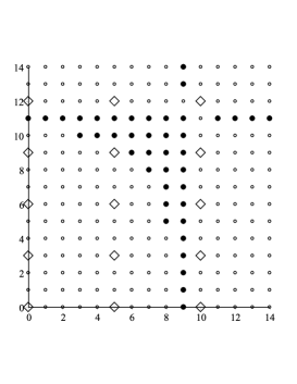
Figure 1: The situation in Example 2.

It is possible to give a proof of Theorem 7 which as a main tool uses Theorem 2 and Proposition 3 in combination with a study of the shape of $U(q,m-1,n)$. Using this approach the proof of the “if” part becomes straight forward whereas the proof of the “only if” part becomes technical and requires more care. Instead of stating the technical proof of the “only if” part we shall present a self contained proof of the “only if” part based on the technique from [3]. Our proof calls for the following lemma which has some interest in itself. We state the lemma in a slightly more general version than shall be needed (we will employ the lemma with ${\mathbb{F}}={\mathbb{F}}_{q}$ and $A_{1}=\cdots=A_{n}={\mathbb{F}}_{q}^{\ast}$).

Lemma 8

Given a field ${\mathbb{F}}$ let $A_{1},\ldots,A_{n}\subseteq{\mathbb{F}}$ be finite sets. Consider proper subsets $B_{1}\subsetneq A_{1},\ldots,B_{n}\subsetneq A_{n}$ and write

$$P(\vec{X})=\prod_{i=1}^{n}\prod_{x\in B_{i}}(X_{i}-x).$$

Assume that $G(\vec{X})\in{\mathbb{F}}[\vec{X}]$ is a polynomial with $\deg_{X_{i}}G<|A_{i}|$, $i=1,\ldots,n$ such that

$$\{\vec{x}\mid\vec{x}\in A_{1}\times\cdots\times A_{n},F(\vec{x})=0\}\subseteq\{\vec{x}\mid\vec{x}\in A_{1}\times\cdots\times A_{n},G(\vec{x})=0\}.$$

Then $F(\vec{X})$ divides $G(\vec{X})$.

Proof: It is enough to prove that $(X_{s}-x)$ divides $G(\vec{X})$ for arbitrary $s\in\{1,\ldots,n\}$ and $x\in B_{s}$. We can write $G(\vec{X})=Q(\vec{X})(X_{s}-x)+R(\vec{X})$ where $R(\vec{X})$ is a polynomial in ${\mathbb{F}}[X_{1},\ldots,X_{s-1},X_{s+1},\ldots,X_{n}]$ and where $\deg_{X_{i}}R<|A_{i}|$ for $i\in\{1,\ldots,s-1,s+1,\ldots,n\}$. We observe that $(\alpha_{1},\ldots,\alpha_{s-1},x,\alpha_{s+1},\ldots,\alpha_{n})$ is a root of $P$ and thereby also of $G$, for all $(\alpha_{1},\ldots,\alpha_{s-1},\alpha_{s+1},\ldots,\alpha_{n})$ in $A_{1}\times\cdots\times A_{s-1}\times A_{s+1}\times\cdots\times A_{n}$. But then $(\alpha_{1},\ldots,\alpha_{s-1},\alpha_{s+1},\ldots,\alpha_{n})$ is a root of $R$ and from the Chinese remainder theorem it follows that $R(\vec{X})=0$.

We are now ready to prove Theorem 7.

Proof: Assume that there exists an $X_{1}^{k_{1}}\cdots X_{n}^{k_{n}}$ with $0<k_{1},\ldots,k_{n}<q-1$ such that (4) holds true. Write

$$G(\vec{X})=X_{1}^{k_{1}}\cdots X_{n}^{k_{n}}P(\vec{X}){\mbox{ mod }}\{X_{1}^{q-1}-1,\ldots,X_{n}^{q-1}-1\}.$$

Clearly the roots of $P(\vec{X})$ in $({\mathbb{F}}_{q}^{\ast})^{n}$ are also roots of $G(\vec{X})$. Hence, by Lemma 8, $G(\vec{X})=Q(\vec{X})P(\vec{X})$ for some $Q(\vec{X})\in{\mathbb{F}}_{q}[\vec{X}]$. Recall that $X_{1}^{s_{1}}\cdots X_{n}^{s_{n}}$ is the leading monomial of $P(\vec{X})$. If we consider a monomial $N$ such that $NX_{1}^{s_{1}}\cdots X_{n}^{s_{n}}\in{\mathcal{M}}(q,n)$ then either $N=1$ or $NX_{1}^{s_{1}}\cdots X_{n}^{s_{n}}\in U(q,m-1,n)$. From assumption (4) it therefore follows that $G(\vec{X})=\alpha P(\vec{X})$ for some $\alpha\in{\mathbb{F}}_{q}^{\ast}$. This implies that

$$P(\vec{X})(X_{1}^{k_{1}}\cdots X_{n}^{k_{n}}-\alpha)=0{\mbox{ mod }}\{X_{1}^{q-1}-1,\ldots,X_{n}^{q-1}-1\}.$$

However, then all non-roots of $P(\vec{X})$ in $({\mathbb{F}}_{q}^{\ast})^{n}$ – that is the elements of $T_{1}\times\cdots\times T_{n}$ – must be roots of $X_{1}^{k_{1}}\cdots X_{n}^{k_{n}}-\alpha$. In other words, for $\vec{x}\in T_{1}\times\cdots\times T_{n}$ we have $x_{i}^{k_{i}}=\alpha_{i}$, $i=1,\ldots,n$ where $\prod_{i=1}^{n}\alpha_{i}=\alpha$. Consider an $i$ such that $t_{i}>1$. Let $y$ and $z$ be two different elements in $T_{i}$. For fixed $x_{j}\in T_{j}$, $j\in\{1,\ldots,i-1,i+1,\ldots,n\}$ both $(x_{1},\ldots,x_{i-1},y,x_{i+1},\ldots,x_{n})$ and $(x_{1},\ldots,x_{i-1},z,x_{i+1},\ldots,x_{n})$ satisfy that they produce the value $\alpha$ when plugged into $X_{1}^{k_{1}}\cdots X_{n}^{k_{n}}$. Hence, $\alpha_{1},\ldots,\alpha_{n}$ are unique. Let $H_{i}=\{\beta\in{\mathbb{F}}_{q}^{\ast}\mid\beta^{k_{i}}=1\}$ (which is a proper subgroup of ${\mathbb{F}}_{q}^{\ast}$ as $0<k_{i}<q-1$), and $\gamma_{i}\in T_{i}$. Then $T_{i}\subseteq\gamma_{i}H_{i}$.
We next prove the “if” part of the theorem. Assume that $T_{i}\subseteq\gamma_{i}H_{i}$, $i=1,\ldots,n$ and write $d_{i}=|H_{i}|$. Define

$$W_{i}=\big{\{}X_{i}^{v}\mid v\in\{jd_{i},\ldots,jd_{i}+(d_{i}-t_{i})\mid j=0,\ldots,\frac{q-1}{d_{i}}-1\}\big{\}}$$

and

$$W=\{X_{1}^{v_{1}}\cdots X_{n}^{v_{n}}\mid X_{i}^{v_{i}}\in W_{i},i=1,\ldots,n\}.$$

Proposition 3 tells us that $\mbox{Supp}P\subseteq W$ and by inspection we find that $U(q-1,m-1,n)$ is contained in ${\mathcal{M}}(q,n)\backslash W$. By symmetry we have

$$X_{1}^{k_{1}}\cdots X_{n}^{k_{n}}W{\mbox{ mod }}\{X_{1}^{q-1}-1,\ldots,X_{n}^{q-1}-1\}=W$$

for all $(k_{1},\ldots,k_{n})$ where for $i=1,\ldots,n$, $k_{i}=\ell_{i}d_{i}$ for some $\ell_{i}$. The theorem follows.

References

[1]
D. A. Cox, J. Little, and D. O’Shea.
Ideals, varieties, and algorithms: an introduction to
computational algebraic geometry and commutative algebra.
Springer, 2nd edition, 1997.
[2]
T. Høholdt.
On (or in) Dick Blahut’s ’footprint’.
Codes, Curves and Signals, pages 3–9, 1998.
[3]
S. Kopparty and Q. Wang.
Roots and coefficients of polynomials over finite fields.
Finite Fields and Their Applications, 29:198–201, 2014.