Power law condition for stability
of Poisson hail

Abstract.

The Poisson hail model is a space-time stochastic system introduced by Baccelli and Foss [BF] whose stability condition is non-obvious owing to the fact that it is a spatially infinite. Hailstones arrive at random points of time and are placed in random positions of space. Upon arrival, if not prevented by previously accumulated stones, a stone starts melting at unit rate. When the stone sizes have exponential tails then stability conditions exist. In this paper, we look at heavy tailed stone sizes and prove that the system can be stabilized when the rate of arrivals is sufficiently small. We also show that the stability condition is, in a weak sense, optimal. We use techniques and ideas from greedy lattice animals.

MSC 2010: 82B44, 82D30, 60K37

Keywords: Poisson hail, stability, workload, greedy lattice animals

1. Introduction

The purpose of this article is to loosen conditions for stability in the “Poisson hail” interacting queueing model introduced by [BF]. In the discrete setting for this model, there are countably many jobs (identified by countably many points in space-time). Job $i$ requires service $\tau_{i}$ from a subset $B_{i}\subset\mathbb{Z}^{d}$. As in the preceding paper, we associate to a job $i$ a (semi-arbitrary) server $x=x(i)\in\mathbb{Z}^{d}$ who is in some sense central in the group $B_{i}$. We suppose that for each site $w\in\mathbb{Z}^{d}$ the jobs $i$ with $x(i)=w$ arrive according to a Poisson process $N_{w}$ of rate $\lambda$. The jobs $i$ arriving at $w$ will have their subsets $B_{i}$ and service times $\tau_{i}$ distributed as i.i.d. vectors, so the arrivals at site $w$ may be considered as a marked Poisson process $\Phi_{w}$. In other words, $\Phi_{w}$ is a Poisson process on $\mathbb{R}\times\mathbb{R}_{+}\times 2^{\mathbb{Z}^{d}}$. Points in its support are typically denoted by $(t,\tau,B)$, the $t$’s forming the aforementioned rate-$\lambda$ Poisson process. The pair $(\tau,B)$ is referred to as the mark of the point $t$. We also assume that the $\Phi_{w}$ are obtained as follows: Let, for each $w$, $\widetilde{\Phi}_{w}$ be an independent copy of $\Phi_{0}$. Then let $\Phi_{w}$ contain all points of the form $(t,\tau,B+w)$ where $(t,\tau,B)$ is a point of $\widetilde{\Phi}_{w}$. Thus, the arrival process (including marks) is translation invariant. Physically, we can think of the system as a model of hailstones of cylindrical shape $B\times[0,\tau]\subset\mathbb{Z}^{d+1}$, where $\tau$ is the height of the stone and $B$ its base. When a hailstone appears at some point of time at which all sites $w\in B$ are free, it starts melting at rate $1$. If there is at least one $w\in B$ occupied by a previously arrived stone, then the current stone will not start melting before all sites in $w$ become free; at the first moment of time this happens, the hailstone starts melting at rate $1$. (Only the ground, $\mathbb{Z}^{d}$ is hot and heat is not transmitted upwards!) At each time $t$, we let $W(t,x)$ be the total work required for $x$ to be free of hailstones provided no stones arrive after $t$. In queueing terms, $W(t,x)$ is a workload. In hailstone terms, $W(t,x)$ is the sum of the heights of all hailstones which contain $x$ in their base and have not been melted yet. Since the superposition of $N_{w}$, $w\in\mathbb{Z}^{d}$, has infinite rate, it follows that within any time interval of positive length there are infinitely many stones arriving. Thus $W(t,\cdot)$ will change infinitely many times in any right neighborhood of $t$. However, typically, for fixed $x\in\mathbb{Z}^{d}$, and any $\varepsilon>0$, $W(t,x)$ depends only on $W(t-\varepsilon,y)$, for $y$ ranging in a finite (but random) number of sites. This is due to the fact that the only have to look at those $\Phi_{w}$ with points $(s,\tau,B)$ such that $t-\varepsilon\leq s\leq t$ and $x\in B$.

Fix $x\in\mathbb{Z}^{d}$ and suppose there is $w\in\mathbb{Z}^{d}$ such that $(t,\tau,B)$ is a point of $\Phi_{w}$. Then

(1) $$W(t+,x)=\begin{cases}\max_{y\in B}W(t-,y)+\tau,&x\in B\\ W(t-,x),&x\not\in B.\end{cases}$$

By convention, we shall assume that $t\mapsto W(t,x)$ is right-continuous: $W(t,x)$ $=W(t+,x)$. On the other hand, if there is no $w$ such that $(t,\tau,B)$ is a point of $\Phi_{w}$ with $x\in B$ then $W(s,t)$, $s\geq t$, decreases linearly for a interval of positive length until either it reaches zero or there is job arriving at some $s>t$ at some site $w$ whose base contains $x$. We have thus completely specified the dynamics of the system. The system considered here differs from that of [KB] in that the latter (i) considers only finitely many sites ($\mathbb{Z}^{d}$ is replaced by a finite set) but (ii) works for stationary and ergodic arrival processes.

The system is said to be stable if (starting from full vacancy at time $0$) the distribution of $W(t,x)$ is tight as $t$ varies for fixed $x$. The central question to be addressed is when is the system stable (for $\lambda$ sufficiently small). More precisely, for which laws on $(\tau,B)$ for jobs arriving at the origin is it the case that there exists $\lambda_{0}\in(0,\infty)$ so that the system is stable for all arrival rates $\lambda<\lambda_{0}$. To avoid trivialities, we assume that $B$ is a finite set, a.s. . The founding article [BF] showed that the system was indeed stable provided that there is $c\in(0,\infty)$ so that

$$\mathbb{E}[e^{c(\tau+(\operatorname{diam}B)^{d})}]<\infty,$$

where $\operatorname{diam}B$ is the diameter of set $B$, i.e., the maximum of $|x-y|_{\infty}$ over all $x,y\in B$, and where $|x|_{\infty}:=\max_{1\leq i\leq d}|x_{i}|$. The proof in [BF] is based on a comparison with an auxiliary branching process with weights requiring the condition stated in the last display.

Our purpose in this paper is to slacken this condition to the existence of the $(d+1+\varepsilon)$-th moment for $\tau+\operatorname{diam}B$. We then (easily) show that this condition is (in a certain weak sense) almost optimal. The key idea is to use ideas on laws of large numbers for lattice animals. This was first proved in [CGGK], though for this paper we take as reference the article by James Martin [JM]. In analogy to [KB], one could also ask whether stability is possible for more general arrival processes. This question, however, is outside the scope of our paper as our method explicitly uses the Poissonian assumptions.

Our principal result is

Theorem 1.

Suppose there exists $\varepsilon>0$ such that $\tau$ and $\operatorname{diam}B$ have finite moments of order $(d+1+\varepsilon)$:

$$\mathbb{E}\tau^{d+1+\varepsilon}+\mathbb{E}(\operatorname{diam}B)^{d+1+\varepsilon}<\infty.$$

Then there exists $\lambda_{0}>0$ so that for job arrival rate $\lambda<\lambda_{0}$ the system is stable.

That this result is (in a weak sense) the best possible is shown by

Theorem 2.

For any $d+1>\varepsilon>0$, we can find a (spatially homogeneous) job arrival process so that

$$\mathbb{E}\tau^{d+1-\varepsilon}+\mathbb{E}(\operatorname{diam}B)^{d+1-\varepsilon}<\infty$$

and the system is unstable.

Remark 1.

The condition of Theorem 1 is equivalent to the following: there exists $\varepsilon>0$ and $C>0$ such that, for any $x\geq 0$,

(2) $$\mathbb{P}(\tau+\operatorname{diam}B>x)\leq\frac{C}{x^{d+1+\varepsilon}}.$$

Similarly, the condition of Theorem 2 is equivalent to the same thing with $-\varepsilon$ in place of $\varepsilon$.

Given stability, it is easy to see that starting from complete vacancy (that is, no workload at any site), the system converges in distribution to an explicitly describable equilibrium. It is natural to ask whether the system possesses other, not necessarily spatially homogeneous, equilibria. While not definitively answering this we show

Theorem 3.

Under the conditions of Theorem 1, there exists $\lambda_{0}>0$ so that for arrival rate $0<\lambda<\lambda_{0}$, the only equilibrium for the system that is spatially translation invariant is the limit measure obtained by starting from zero workload.

We now assemble some observations and techniques from earlier papers, [KB, BF]. Start the system at time $-n$ from full vacancy and consider how the workload $W^{n}(t,x)$ at time $t\geq-n$ and site $x\in\mathbb{Z}^{d}$ is obtained.

Definition 1.

Let $\Gamma^{n}(x,t)$ be the set of locally constant cadlag (= piecewise constant, continuous on the right with left limits at every point) paths $\gamma:[u,t]\rightarrow\mathbb{Z}^{d}$ for some $-n\leq u\leq t$ such that
(i) $\gamma(t)=x$,
(ii) if $\gamma(s)\neq\gamma(s-)$, then a job arrived at time $s$ requiring service from both servers $\gamma(s)$ and $\gamma(s-)$.

Associate to such a $\gamma\in\Gamma^{n}(x,t)$ the score

$$V(\gamma)=\sum_{i}\tau_{i}-(t-u),$$

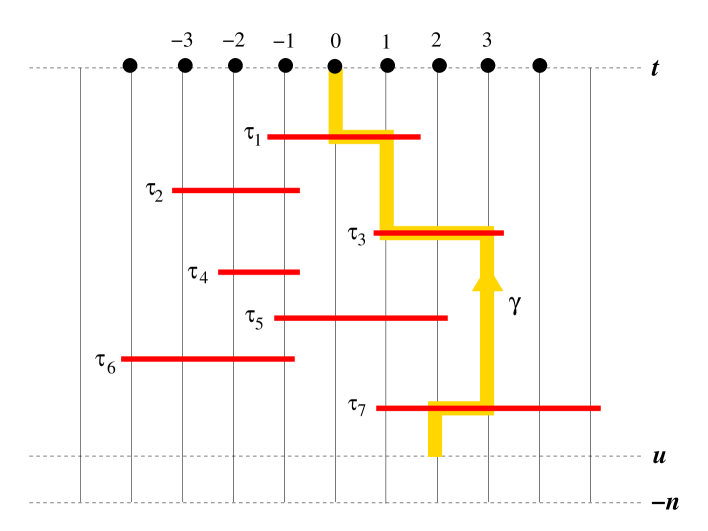
Figure 1. Graphical representation of the part of the process responsible for the computation of the profile $W(t,\cdot)$ when the system starts with $W(-n,\cdot)\equiv 0$. Consider the evaluation of $W(t,0)$ at site $x=0$. Horizontal intervals represent hailstone (job) arrivals with heights $\tau_{i}$. Only those arrivals which can potentially influence $W(t,0)$ are shown. Consider a path $\gamma$ as indicated, from $(u,2)$ to $(t,0)$. Its score is $V(\gamma)=\tau_{1}+\tau_{3}+\tau_{7}-(t-u)$. $W(t,0)$ is the maximum of these scores over all such paths starting from some $(u,y)$ and ending at $(t,0)$.

where the sum is over jobs $(\tau_{i},B_{i})$ which are arrive at time $s_{i}$ with $\gamma(s_{i})\in B_{i}$. Based on the way that the workload evolves (see discussion around equation (1)) we obtain that $W^{n}(t,x)=\sup_{\gamma\in\Gamma^{n}(x,t)}V(\gamma)$. See Figure 1.

There are three monotonicity properties that the system possesses and which we take into account when analyzing its stability. We start from full vacancy at time $-n$ and consider $W^{n}(t,x)$ for some $t\geq-n$. Then $W^{n}(t,x)$ will increase if we (i) delay all arrivals between $-n$ and $t$, or (ii) increase the heights of the stones, or (iii) enlarge their bases.

Thanks to the monotonicity, it was deduced in [BF] that it is enough, for the results sought, to consider the case where the sets $B$ for the team of servers required for a job $i$ with $x(i)=0$ is a cube centred at the origin and we write (for a job arriving at server $x$ in time interval $(m-1,m]$) $R^{x,m}_{i}$ for the value so that $B=x+[-R^{x,m}_{i},R^{x,m}_{i}]^{d}$. We will work with time doubly infinite, notwithstanding the fact that we consider the process on $[-n,\infty)$.

The first step is the discretization of the Poisson processes. We consider for $m\in\mathbb{Z}$ and $x\in\mathbb{Z}^{d}$ the random variables

$$R_{x,m}=\sum_{i}R^{x,m}_{i},\quad T_{x,m}=\sum_{i}\tau^{x,m}_{i},$$

the sum taken over all jobs $i$ arriving on the time interval $(m-1,m]$ at site $x$. Since the summands in $R_{x,m}$ are i.i.d. and their number is Poisson (and, therefore, light-tailed), it is clear that $R_{x,m}$ has finite $\alpha$ moment if each summand has finite $\alpha$ moment. Similarly for $T_{x,m}$.

Lemma 4.

If for $\alpha>0$, $\mathbb{E}(\operatorname{diam}B)^{\alpha}<\infty$ (resp., $\mathbb{E}\tau_{i}^{\alpha}<\infty$), then $\mathbb{E}R_{x,m}^{\alpha}<\infty$ (resp. $\mathbb{E}T_{x,m}^{\alpha}<\infty$).

We will deal with the discretized system where at server $w$ at time $n$ a job requiring service time $T_{w,n}$ from each server in the cube $[w-R_{w,n},w+R_{w,n}]^{d}$. By the monotonicity (see [BF] for detail), this discretization is effective in that if we can show stability for the discretized system of jobs then we will have shown stability for the original system: the workload at time $m$ for this system will dominate that arising from the nondscretized model. It is also as well to note that we have not given up too much here. In principle, if we have multiple $w$ jobs arriving during interval $(m-1,m]$ then we could, again in principle, lose if one job required a long service but only from $w$ while a second job required a very short service from a large cube of servers centred at $w$. However this will be rare for small $\lambda$, where our analysis is most relevant.

2. (Very) greedy lattice animals (GLA)

As noted, we wish to exploit the celebrated results (see [CGGK]) on greedy lattice animal systems. Recall that a lattice animal of $\mathbb{Z}^{r}$ is simply a connected subset (when $\mathbb{Z}^{r}$ is considered as a graph with the standard edge set). We are given a collection of i.i.d. positive random variables $\{X(x)\}_{x\in\mathbb{Z}^{r}}$. We suppose the existence of $\varepsilon>0$ so that $\mathbb{E}X(0)^{r+1+\varepsilon}<\infty$ or, equivalently, the existence of $\varepsilon>0$ and $C<\infty$ so that for all $t>1$,

(3) $$\mathbb{P}(X(0)>t)\leq C/t^{r+1+\varepsilon}.$$

(The $1$ in the power is unnecessary but it is in this case that we will use our results.)

We will then parametrize our system by taking i.i.d. random variables $X^{\lambda}(x)$ to be equal to $X(x)$ with probability $\lambda$ and otherwise $0$. For $\zeta\subset\mathbb{Z}^{r}$, its $X^{\lambda}$ value (or score) is simply

(4) $$X^{\lambda}(\zeta):=\sum_{x\in\zeta}X^{\lambda}(x).$$

The size $|\zeta|$ of the lattice animal is its cardinality. Note that $X^{\lambda}(\zeta)\to 0$, as $\lambda\to 0$, in probability, for any lattice animal of finite size. We fix positive integer $k$ and $c_{1}>0$ and consider the event

$$A_{k}:=\big{\{}\exists\text{ lattice animal $\zeta$ containing $0$},\,|\zeta|=2^{k},\,X^{\lambda}(\zeta)\geq c_{1}2^{k}\big{\}}.$$

We wish to prove the following upper bound on the probability of $A_{k}$, a result which may be of independent interest. We note that $\mathbb{P}(A_{k})$ depends both on $\lambda$ and $c_{1}$.

Proposition 5.

Given any $c_{1}>0$, there exists a $\lambda_{0}>0$ and a function $C:[0,\lambda_{0})\to(0,\infty)$ so that $C(\lambda)\rightarrow 0$ as $\lambda\rightarrow 0$ and so that, for $\lambda<\lambda_{0}$ and for all positive integers $k$,

$$\mathbb{P}(A_{k})\leq\frac{C(\lambda)}{2^{k(1+\varepsilon)}}.$$

Remark 2.

(i) We can use the above to bound the probability that there is a lattice animal of size $u\geq 2^{k}$ containing the origin whose value is $\geq c_{1}u$, when $\lambda$ is small, by considering $\bigcup_{\ell\geq k}A^{c_{1}/2}_{\ell}$ whose probability, by the above, is less than $C(\lambda)2^{-k(1+\varepsilon)}(1-2^{-(1+\varepsilon)})^{-1}$.
(ii) The above formalism will certainly apply to our situation with random variables $R_{x,m}+T_{x,m}$ at each site $x\in\mathbb{Z}^{r}$. Indeed, if $X(x)$ denotes the random variable at site $x$ for rate $\lambda=1$ conditioned on there being at least one arrival, then it is easy to see that with rate $\lambda<1$, $R_{x,m}+T_{x,m}$ is stochastically less than $X^{1-e^{-\lambda}}(x)$.

Some notation used in the proof and elsewhere. If $x=(x_{1},\ldots,x_{r})\in\mathbb{R}^{r}$ then $|x|_{\infty}:=\max_{1\leq i\leq r}|x_{r}|$. The $L^{\infty}$ ball $\mathbb{B}(x,\rho)$ centred at $x$ is the set

$$\mathbb{B}(x,\rho)=\{y\in\mathbb{R}^{r}:\,|y-x|_{\infty}\leq\rho\}.$$

We also let $|x|_{1}:=\sum_{i=1}^{r}|x_{i}|$. We use ${\text{\Large$\mathfrak{1}$}}_{A}$ for the indicator of $A$.

Proof of Proposition 5.

We split the value $X^{\lambda}(\zeta)$, see equation (4), into three parts:

(5) $$X^{\lambda}(\zeta)=X^{\lambda}_{a}(\zeta)+X^{\lambda}_{b}(\zeta)+X^{\lambda}_{c}(\zeta),$$

where

$$X^{\lambda}_{a}(\zeta) :=\sum_{x\in\zeta}X^{\lambda}(x)\,{\text{\Large$\mathfrak{1}$}}_{X^{\lambda}(x)\leq 2^{qk}/k^{2}}$$

$$X^{\lambda}_{b}(\zeta) :=\sum_{x\in\zeta}X^{\lambda}(x)\,{\text{\Large$\mathfrak{1}$}}_{2^{qk}/k^{2}<X^{\lambda}(x)\leq 2^{vk}}$$

$$X^{\lambda}_{c}(\zeta) :=\sum_{x\in\zeta}X^{\lambda}(x)\,{\text{\Large$\mathfrak{1}$}}_{X^{\lambda}(x)>2^{vk}}.$$

The constants $q$ and $v$ appearing in the splitting are chosen as

$$q:=\frac{r}{r+1+\varepsilon}<v<1.$$

Define next four events:

$$A_{k,a} :=\big{\{}\exists\text{ lattice animal $\zeta$ containing $0$},\,|\zeta|=2^{k},\,X^{\lambda}_{a}(\zeta)\geq c_{1}2^{k}/10\big{\}}$$

$$A_{k,b} :=\big{\{}\exists\text{ lattice animal $\zeta$ containing $0$},\,X^{\lambda}_{b}(\zeta)\geq c_{1}2^{k}/10\big{\}}$$

$$A_{k,c} :=\big{\{}N^{\lambda}_{c}(B_{k})\geq m\big{\}}$$

$$A_{k,d} :=A_{k}\setminus(A_{k,a}\cup A_{k,b}\cup A_{k,c}),$$

where $m$ is a positive integer satisfying

(6) $$m(v(r+1+\varepsilon)-r)>1+\varepsilon,$$

where $B_{k}:=[-2^{k},2^{k}]^{r}=\mathbb{B}(0,2^{k})$, and where $N^{\lambda}_{c}(B_{k})$ is the integer-valued random variable

$$N^{\lambda}_{c}(B_{k}):=\sum_{x\in B_{k}}{\text{\Large$\mathfrak{1}$}}_{X^{\lambda}(x)>2^{vk}}.$$

Note that if a lattice animal $\zeta$ of size $|\zeta|=2^{k}$ contains $0$, then $\zeta\subset B_{k}$.

We obtain an upper bound for $\mathbb{P}(A_{k})$ via

$$\mathbb{P}(A_{k})\leq\mathbb{P}(A_{k,a})+\mathbb{P}(A_{k,b})+\mathbb{P}(A_{k,c})+\mathbb{P}(A_{k,d}).$$

Bound for $\mathbb{P}(A_{k,d})$: Since $A_{k}$ occurs, there is a lattice animal $\zeta$ of size $2^{k}$ containing the origin and having value $X^{\lambda}(\zeta)\geq c_{1}2^{k}$. Since $A_{k,a}$ does not occur, we have $X^{\lambda}_{a}(\zeta)\leq c_{1}2^{k}/10$. Since $A_{k,b}$ does not occur, we have $X^{\lambda}_{b}(\zeta)\leq c_{1}2^{k}/10$ and so $X^{\lambda}_{b}(\zeta)\leq c_{1}2^{k}/10$. Therefore, from (5),

$$X^{\lambda}_{c}(\zeta)\geq\frac{c_{1}2^{k}}{2}.$$

But this, together with the fact that $A_{k,c}$ does not occur, implies that there is $x\in B_{k}$ such that $X^{\lambda}_{x}\geq 2^{k}c_{1}/2m$. Hence

$$\mathbb{P}(A_{k,d})\leq\sum_{x\in B_{k}}\mathbb{P}(X^{\lambda}(x)\geq 2^{k}c_{1}/2m)\leq K_{m}\lambda/2^{(1+\varepsilon)k},$$

for some constant $K_{m}$.

Bound for $\mathbb{P}(A_{k,c})$: The event $A_{k,c}$ is the event that the sum of at most $(2\times 2^{k}+1)^{r}$ Bernoulli random variables, each taking value $1$ with probability at most $p_{k}=\lambda C2^{-kv(r+1+\varepsilon)}$, exceeds $m$. To bound this probability we observe that if $S_{n}(p)$ is the sum of $n$ i.i.d. Bernoulli$(p)$ random variables then $\mathbb{P}(S_{n}(p)\geq m)$ is upper bounded by the probability that there is a set $A\subset\{1,\ldots,n\}$ of size $m$ such that all Bernoulli random variables are equal to $1$ on $A$, so

(7) $$\mathbb{P}(S_{n}(p)\geq m)\leq\binom{n}{m}p^{m}\leq\frac{n^{m}p^{m}}{m!}.$$

$$\mathbb{P}(A_{k,c})\leq\big{(}(2^{k+1}+1)^{r}p_{k}\big{)}^{m}\leq\frac{K_{m}^{\prime}\lambda}{2^{(1+\varepsilon)k}},$$

for some constant $K_{m}^{\prime}$ and thanks to the choice (6) for $m$.

Bound for $\mathbb{P}(A_{k,b})$: We have

$$\mathbb{P}(A_{k,b}) =\mathbb{P}\left(\exists\text{ lattice animal }\zeta,\,\sum_{x\in\zeta\cap B_{k}}X^{\lambda}(x){\text{\Large$\mathfrak{1}$}}_{2^{qk}/k^{2}<X^{\lambda}(x)\leq 2^{vk}}\geq\frac{c_{1}2^{k}}{10}\right)$$

$$\leq\mathbb{P}\left(2^{vk}\sum_{x\in B_{k}}{\text{\Large$\mathfrak{1}$}}_{2^{qk}/k^{2}<X^{\lambda}(x)\leq 2^{vk}}\geq\frac{c_{1}2^{k}}{10}\right)$$

$$\leq\mathbb{P}\left(\sum_{x\in B_{k}}{\text{\Large$\mathfrak{1}$}}_{2^{qk}/k^{2}<X^{\lambda}(x)}\geq\frac{c_{1}2^{(1-v)k}}{10}\right)$$

The sum in the probability is the sum of $n_{k}=(2^{k+1}+1)^{r}$ Bernoulli random variables, each with probability being 1 being at most $p_{k}:=\lambda C(2^{qk}/k^{2})^{-(r+1+\varepsilon)}=\lambda Ck^{2(r+1+\varepsilon)}/2^{rk}$. We can apply now inequality (7) with $n=n_{k}$, $p=p_{k}$ and $m=c_{1}2^{k(1-v)}/10$, and the Stirling formula for $m!\sim\sqrt{2\pi m}e^{m(\log m-1)}$, to obtain that the required probability $\mathbb{P}(A_{k,c})$ is not bigger than

$$\lambda e^{-m(\log m-2(r+1+\varepsilon)\log k)(1+o(1))}=\lambda o\left(2^{-(1+\varepsilon)k}\right),$$

as $k\to\infty$. Therefore,

$$\mathbb{P}(A_{k,c})\leq\frac{K^{\prime\prime}\lambda}{2^{(1+\varepsilon)k}},$$

for some constant $K^{\prime\prime}$.

Bound for $\mathbb{P}(A_{k,a})$: We repeat the argument given in [JM] (or [CGGK]).

Lemma 6 (Lemma 1 in [CGGK], Lemma 2.1 in [JM]).

For any lattice animal $\zeta$ of size $n$ containing the origin and any $1\leq\ell\leq n$ we can find a sequence $0=u_{0},u_{1},\ldots,u_{h}$ of points in $\mathbb{Z}^{r}$, $h$ being the integer part of $2n/\ell$, and $|u_{i}-u_{i-1}|_{\infty}\leq 1$ for all $1\leq i\leq h$, so that

$$\zeta\subset\bigcup_{i=0}^{h}\mathbb{B}(\ell u_{i},2\ell).$$

Proof.

For $y=(y^{1},\ldots,y^{r})\in\mathbb{R}^{r}$, let $\lfloor y/\ell\rfloor$ be the point $x$ in $\mathbb{Z}^{r}$ such that $x^{i}=\lfloor y^{i}/\ell\rfloor$ (the quotient of the division by $\ell$, componentwise). Clearly, $\ell x\leq y<\ell(x+1)$, componentwise, so $|y-\ell x|_{\infty}\leq\ell$. If $\zeta$ is a lattice animal containing $0$ we can find a sequence $\pi=(\pi_{0},\ldots,\pi_{2n})$ such that successive elements are either identical or neighbors in $\mathbb{Z}^{r}$ ($\pi$ is a path) and such that $\{\pi_{0},\ldots,\pi_{2n}\}=\zeta$. (To do this, consider a spanning tree of $\zeta$ and form $\pi$ by traversing the tree “from the bottom”.) Then $|\pi_{i}-\pi_{j}|_{\infty}\leq\ell$ if $|i-j|\leq\ell$. Define $u_{i}\in\mathbb{Z}^{r}$ by $u_{i}:=\lfloor\pi_{i\ell}/\ell\rfloor$, $i=0,\ldots,h$. Then $|u_{i}-u_{i-1}|_{\infty}\leq\ell$ for all $i$. Furthermore, if $x\in\zeta$ then $x=\pi_{t}$ for some $0\leq t\leq 2n$. Let $k=\lfloor t/\ell\rfloor$. Then $|\pi_{t}-\ell u_{k}|_{\infty}\leq|\pi_{t}-\pi_{k\ell}|_{\infty}+|\pi_{k\ell}-\ell u_{k}|_{\infty}\leq\ell+\ell$, so $x=\pi_{t}\in\mathbb{B}(\ell u_{k},2\ell)$. ∎

From this it is immediate that for given $\ell$ there are at most $9^{r2n/\ell}$ such $2\ell$–ball coverings. We use this result with $n=2^{k}$ . We consider $\ell$ of “scale” $2^{i}$ with $2^{i}\leq 2^{qk}/k^{2}$. Let $i_{0}$ be the maximal such value. For given $i$, we choose the value $\ell=l(i)$ to equal the integer part of $\lambda^{-1/2r}\,2^{i/q}$. With this value the probability that a $L^{\infty}$ ball of radius $2\ell$ contains a site having an $X^{\lambda}$ value is small for $\lambda$ small but not (in principle) negligible. From this it is easily seen that given a sequence $u_{0},u_{1},\ldots,u_{h}$ satisfying the above (and therefore given an $\ell$ covering), the probability that

the number of sites within the covering having value at least $$2^{i} 2(2^{k}/\ell)c_{1}$$ is at least

is bounded above by $20^{-2r\cdot 2^{k}/\ell}$ for $\lambda$ small. Thus we see that outside an event of probability $9^{hr}20^{-2\cdot 2^{k}r/\ell}$, this bound will hold for all $\ell$–coverings. Summing over $i$ such that $2^{i}\leq 2^{kq}/k^{2}$ we have that outside probability

$$\sum_{2^{i}\leq 2^{kq}/k^{2}}(\frac{1}{2}){2\cdot 2^{k}r/\ell(i)}\leq 2(\frac{1}{2})^{2\cdot 2^{k}r/\ell(i_{0})}\leq 2(\frac{1}{2})^{c(\lambda k^{2/q})}$$

for each such $i$ and for each corresponding $\ell(i)$–covering, the number of sites in the covering whose $X^{\lambda}$ value at least $2^{i}$ is at most $2(2^{k}/\ell)c_{1}$.

Thus (outside of probability $2(\frac{1}{2})^{c(\lambda k^{2/q})}$ for some universal $c$) we have, for any lattice animal $\zeta$ of size $2^{k}$,

$$\sum_{x\in\zeta}X^{\lambda}(x){\text{\Large$\mathfrak{1}$}}_{X^{\lambda}(x)\leq\frac{2^{k(r+1+\varepsilon)/d}}{k^{2}}}\leq\sum_{i\leq i_{0}}2(2^{k}/\ell(i))\,c_{1}2^{i+1}\leq\sum_{i\leq i_{0}}4\cdot 2^{k}\lambda^{1/2r}2^{-i(1+\varepsilon)/r}$$

which is bounded by $\text{Constant}(\varepsilon)2^{k}\lambda^{(1+\varepsilon)/2r}$. The conclusion follows for large $k$. Thus we have shown the proposition. ∎

Corollary 7.

Define

$$B^{c_{1}}_{u}(x):=\{\exists\text{ lattice animal $\zeta$ containing $x$,\, $|\zeta|\geq u$,\, $X^{\lambda}(\zeta)\geq c_{1}|\zeta|$}\}.$$

For $c_{1}<1$ fixed, there exists a constant $\lambda_{1}=\lambda_{1}(c_{1})$ and a function $H$ defined on $[0,\lambda_{1})$ tending to zero as $\lambda$ tends to zero, so that for all $0<\lambda<\lambda_{1}$ and all positive integers $R$,

$$\mathbb{P}\left(\bigcup_{x\in[-R,R]^{r}}B^{c_{1}}_{u}(x)\right)\leq\begin{cases}\displaystyle\frac{H(\lambda)}{{(u+1)}^{1+\varepsilon}},&u\geq R\\ \displaystyle\frac{H(\lambda)R^{r}}{{(u+1)}^{r+1+\varepsilon}},&u\leq R.\end{cases}$$

Proof.

We treat the case $u\geq R$ only as that for $u\leq R$ is essentially the same. Fix $c_{2}<c_{1}$. Let

$$N=\sum_{x\in[-R,R]^{r}}{\text{\Large$\mathfrak{1}$}}_{B^{c_{2}}_{u}(x)}.$$

By Proposition 5 and Remark 2(i), $\mathbb{P}(B^{c_{2}}_{u}(x))\leq C(\lambda)/2^{k(1+\varepsilon)}$ where $k$ is the largest integer with $2^{k}\leq u$. Therefore

$$\mathbb{E}(N)\leq\frac{C(\lambda)(2R+1)^{r}}{2^{k(1+\varepsilon)}}.$$

Now suppose that event $\bigcup_{x\in[-R,R]^{r}}B^{c_{1}}_{u}(x)$ occurs. Then for some $x\in[-R,R]^{r}$ and some lattice animal $\xi$ containing $x$, $X^{\lambda}(\xi)\geq c_{1}|\xi|$. Now for every $y\in[-R,R]^{r}$ with $|y-x|_{\infty}\leq\frac{R(c_{1}-c_{2})}{c_{2}r}$, we can create a new lattice animal $\xi^{\prime}$ containing both $y$ and $\xi$ by adding at most $(c_{1}-c_{2})R/c_{2}$ points to $\xi$. Since we assumed $R\leq u\leq|\xi|$, we have $|\xi|\leq|\xi^{\prime}|\leq(c_{1}/c_{2})|\xi|$. By positivity of the random variables

$$X^{\lambda}(\xi^{\prime})\geq X^{\lambda}(\xi)\geq c_{1}|\xi|\geq c_{2}|\xi^{\prime}|.$$

Thus the event $\bigcup_{x\in[-R,R]^{r}}B^{c_{1}}_{u}(x)$ is a subset of the event that random variable $N$ defined at the start of the proof is at least $(\frac{(c_{1}-c_{2})R}{rc_{2}})^{r}$. Our result now follows from Markov’s inequality.

∎

3. Cluster formation and their properties

In this section we construct clusters for our Poisson hail corresponding to integer intervals $(m-1,m]$. The clusters themselves will follow a clustering procedure of [BF] and will depend only on the random variables $\{R_{x,m}\}_{x}$. Our departure will consist in the temporal (or workload) variable we associate to each cluster. Our clusters will have the property that if $C\subset\mathbb{Z}^{d}$ is a cluster and $\gamma:(m-1,m]\to\mathbb{Z}^{d}$ is a path satisfying property (ii) of Definition 1, then

(8) $$\gamma(m)\in C\Rightarrow\gamma(s)\in C\text{ for all }s\in(m-1,m].$$

Recall we discretized time by identifying with $m$ all tasks for site $x$ arriving in $(m-1,m]$ with a single task of “radius”

$$R_{x,m}\equiv\sum R_{i}^{x,m},$$

summed over all tasks arriving at $x$ in time interval $[m-1,m]$. We denote by $t^{x,m}_{i}$ the times of the arrivals, i.e., the points of the Poisson process $N_{x}$ in the interval $(m-1,m]$. The indices $i$ are coordinated so that for site $x$ a job arrives at time $t^{x,m}_{i}$ requiring $\tau^{x,m}_{i}$ units of service from servers in $x+[-R_{i}^{x,m},R_{i}^{x,m}]^{d}$.

By Lemma 4,

$$\mathbb{P}(R_{x,m}\geq u)\leq\frac{C}{(u+1)^{d+1+\varepsilon}},$$

for some $\varepsilon>0$ and some finite constant $C=C(\varepsilon)$ for any $\varepsilon$ conforming to the hypotheses of Theorem 1.

For fixed “time” $m$ and $y\in\mathbb{Z}^{d}$ let

$$D_{y,m}:=\mathbb{B}(y,R_{y,m})$$

be the $L^{\infty}$ ball centred at $y$ and having radius $R_{y,m}$. The cluster $C(x,m)$ containing $x$ is defined as the union of such $D_{y,m}$ over $y$ having the property that there exists integer $K$ and sites $y=z_{0},\ldots,z_{K}=x$ such that $D_{z_{i},m}\cap D_{z_{i-1},m}\not=\varnothing$, for all $1\leq i\leq K$.

Let $D(x,m)$ be the diameter of the cluster $C(x,m)$. It is clear that these clusters have the property (8) above. What is not a priori clear is that even with very small rate $\lambda$ the clusters will be a.s. finite. However the preceding section enables us to prove

Lemma 8.

Assume that $\mathbb{P}(X(0)>t)\leq C/t^{d+1+\varepsilon}$.

Then there exists a function $K(\lambda)$ tending to zero as $\lambda$ tends to zero so that, for $\lambda$ sufficiently small and all positive integers $z$,

$$\mathbb{P}(D(0,m)\geq z)\leq\frac{K(\lambda)}{z^{1+\varepsilon}}.$$

Proof.

Consider the GLA system with random variables $\{Z(x)\}_{x\in\mathbb{Z}^{d}}$ for

$$Z(x)=R_{x,m}.$$

If the diameter $D(0,m)$ of the cluster $C(0,m)$ containing the origin exceeds $z$ then there must exist $L$ and $0=x_{0},x_{1},\ldots,x_{L}$ so that, for all $1\leq i\leq L$,

(9) $$|x_{i-1}-x_{i}|_{\infty}\leq R_{x_{i},m}+R_{x_{i-1},m}$$

and $|x_{L}|\geq z$. We choose $\zeta$ to be the lattice animal $\bigcup_{i=1}^{L}P(x_{i-1},x_{i})$ where $P(x_{i-1},x_{i})$ is a path connecting $x_{i-1}$ and $x_{i}$ of length $|x_{i-1}-x_{i}|_{1}$. (Recall that $|x|_{1}$ denotes the $L^{1}$ norm.) Then $\zeta$ is a lattice animal in $\mathbb{Z}^{d}$ containing the origin for which $\sum_{y\in\zeta}Z(y)\geq\sum_{i=0}^{L}Z(x_{i})$. By (9),

$$\sum_{i=0}^{L}Z(x_{i})\geq\frac{1}{2}\sum_{j=1}^{L}|x_{i-1}-x_{i}|_{\infty}\geq\frac{1}{2d}\sum_{j=1}^{L}|x_{i-1}-x_{i}|_{1}\ =|\zeta|/2d\geq z/2d.$$

The result follows from Proposition 5 applied to $c_{1}<\frac{1}{4d}$.

∎

Arguing as in Corollary 7, we obtain

Corollary 9.

There is a function $C(\lambda)$ tending to zero as $\lambda\to 0$ so that for $\lambda$ small, for all $L$, and for $R\leq L/2$,

$$\mathbb{P}(\exists x\in[-R,R]^{d}\text{ with }D(x,m)\geq L)\leq\frac{C(\lambda)}{L^{1+\varepsilon}}.$$

while for $\lambda$ small and $R\geq L/2$

$$\mathbb{P}(\exists x\in[-R,R]^{d}\text{ with }D(x,m)\geq L)\leq\frac{C(\lambda)R^{d}}{L^{d+1+\varepsilon}}.$$

We now consider the “time” $T(x,m)$ associated with the cluster $C(x,m)$. This definition is a little less direct than that for $D(x,n)$: Given $x\in\mathbb{Z}^{d}$ and integer $m$ (and so given cluster $C(x,m)$), $T(x,m)$ is equal to the maximum value of

$$\sum_{i=0}^{L}\tau_{j(i)}^{x_{i},m}$$

over sequences $x_{0},x_{1},\ldots,x_{L}\in C(x,m)$ and $m\geq t_{0}\geq t_{1}\geq\cdots\geq t_{L}\geq{m-1}$ so that, for all $i$ a job arrives at $x_{i}$ at time $t_{i}=t^{x,m}_{j(i)}$ having work time $\tau^{x_{i},m}_{j(i)}$ and

$$|x_{i-1}-x_{i}|_{\infty}\leq R^{x_{i},m}_{j(i)}+R^{x_{i-1},m}_{j(i)},\quad 1\leq i\leq L.$$

We remark that, under the latter two conditions, if $x_{0}\in C(x,m)$ then necessarily the “subsequent” $x_{i}$ are also in this cluster. We note also that this definition (which requires more information than the discretized data) ensures that, for any site in $C(x,m)$, the waiting time accrued during time interval $(m-1,m]$ is less than or equal to $T(x,m)$.

Lemma 10.

There exists function $K(\lambda)$ which tends to zero as $\lambda$ tends to zero so that for $\lambda$ sufficiently small for all $z\geq 1$,

$$\mathbb{P}(T(0,m)\geq z)\leq\frac{K(\lambda)}{z^{1+\varepsilon}}.$$

Proof.

By the previous lemma we may suppose that $D(0,n)\leq z/100$. Again if $T(0,m)$ takes a value exceeding $z$ then there must exist $L$ and a sequence $x_{0},x_{1},\ldots,x_{L}\in C(0,m)$ and times $m\geq t_{0}\geq t_{1}\geq\cdots\geq t_{L}\geq{m-1}$ so that, for all $i\leq L-1$, there is a job arrival at $x_{i}$ at time $t_{i}$ and

$$|x_{i-1}-x_{i}|_{\infty}\leq R^{x_{i},m}_{j(i)}+R^{x_{i-1},m}_{j(i-1)},\quad 1\leq i\leq L,$$

and also $\sum_{i}T(x_{i},t_{i})\geq z$. It is important to note that we do not assume that the $x_{i}$ are distinct. Indeed it is for this reason that we use that bound involving $R^{x_{i},m}_{j(i)}$ rather than $R_{x_{i},m}$. However if $y$ is equal to $x_{i_{1}},x_{i_{2}},\ldots,x_{i_{r}}$, then of course $R_{y,m}\geq\sum_{k}R^{x_{i_{k}},m}_{j(i_{k})}$ and equally $T_{y,m}\geq\sum_{k}\tau^{x_{i_{k}},m}_{j(i_{k})}$. Thus as before we obtain, as in Lemma 8, but with $Z(x)=R_{x,m}+T_{x,m}$, that for a lattice animal $\zeta=\bigcup_{i}P(x_{i-1},x_{i})$ that the GLA$(Z)$ score (i.e. $\sum_{x\in\zeta}(R_{x,m}+T_{x,m})$) will exceed $(z+|\zeta|)/4d$.

∎

Again we have

Corollary 11.

There exists function $C(\lambda)$ which tends to zero as $\lambda$ tends to zero so that for so that for all $L$ and for $R\leq L/2$,

$$\mathbb{P}(\exists x\in[-R,R]^{d}\text{ with }T(x,m)\geq L)\leq\frac{C(\lambda)}{L^{1+\varepsilon}}.$$

while for $\lambda$ small and $R\geq L/2$

$$\mathbb{P}(\exists x\in[-R,R]^{d}\text{ with }T(x,m)\geq L)\leq\frac{C(\lambda)R^{d}}{L^{d+1+\varepsilon}}.$$

4. Workload bounds and stability

We now apply the foregoing to analyze the workload stability for small values of $\lambda$. It is enough to show tightness of the workload $W^{n}(0,0)$ at time $0$ when the system starts empty at time $-n$. Recall that $W^{n}(0,0)$ is obtained as the maximum of scores $V(\gamma)$ where $\gamma$ ranges in the set of paths $\Gamma^{n}(0,0)$. See Definition 1.

Due to the monotonicity properties of the system, $W^{n}(0,0)$ is readily seen to be bounded above by the quantity $W^{n,D}(0,0)$ which corresponds to the discretized system and is given by

$$W^{n,D}(0,0)=\sup_{\gamma}V^{D}(\gamma),$$

where the supremum is taken over discrete time indexed paths paths $\gamma:[-r,0]\rightarrow\mathbb{Z}^{d}$ for some $0\leq r\leq n$ satisfying
(i) $\gamma(0)=0$,
(ii) for each $-n<i\leq 0$, $\gamma(i-1)$ belongs to cluster $C(\gamma(i),i)$.
The score $V^{D}(\gamma)$ of $\gamma$ is given by

$$V^{D}(\gamma)=\left(\sum_{i=0}^{r-1}T(\gamma(-i),-i))\right)-r.$$

We now consider a cube $H$ of length $R$ in $\mathbb{Z}^{d+1}=\mathbb{Z}^{d}\times\mathbb{Z}$ where the first $d$ coordinates are considered as “spatial” and the last one temporal. Accordingly, we write $H$ as $H^{\prime}\times I$ where $I$ is a temporal interval of length $R$ and $H^{\prime}$ is a cube of length $R$ in $\mathbb{Z}^{d}$. We define the variable

$$V(H,u):=\text{number of clusters $C(x,m)$ intersecting $H^{\prime}\times\{m\}$}\\ \text{and having $D(x,m)+T(x,m)\geq u$, $m\in I$.}$$

Clusters are by definition enclosed in a slab $\mathbb{Z}^{d}\times\{m\}$ for some $m$ and the clusters at different temporal levels $m$ are independent. Thus (after repeated use of Lemma 2 of [BF]) we easily obtain from Corollaries 9 and 11.

Proposition 12.

There exists constant $K_{\lambda}$ so that, for $u\leq R$, $V(H,u)$ is stochastically less than Poisson of parameter $\frac{K_{\lambda}R^{d+1}}{{(u+1)}^{d+1+\varepsilon}}$. For $u\geq R$ it is bounded by a Poisson of parameter $\frac{K_{\lambda}R}{{(u+1)}^{1+\varepsilon}}$. Furthermore, as $\lambda$ tends to zero, $K_{\lambda}$ tends to zero.

Given the above for $C$ a cluster corresponding to temporal interval $(m-1,m]$, we define a value $X_{m}(C)$ to signify the value $D(x,m)+T(x,m)$ for a (and so any) $x$ in $C$.

In analyzing $V^{D}(\gamma)$ we will consider a (nonstandard) lattice animal system on $\mathbb{Z}^{d+1}$. Instead of having i.i.d. random variables indexed by points $(x,m)\in\mathbb{Z}^{d+1}$, we will consider a lattice animal model based on the random variables $X_{m}(C)$ which, while independent for distinct collections of index $m$, are not independent. Given a lattice animal $\Xi\subset\mathbb{Z}^{d+1}$, we write $\Xi_{m}$ to denote $\Xi\cap\mathbb{Z}^{d}\times\{m\}$ ( of course in general $\Xi_{m}$ will not be a lattice animal). Obviously given $\Xi$, all but finitely many $\Xi_{m}$ will be empty. The value $V^{C}(\Xi)$ associated with such a lattice animal $\Xi$ will be

$$V^{C}(\Xi):=\sum_{m\in\mathbb{Z}}\,\sum_{C\text{ cluster in }\mathbb{Z}^{d}\times\{m\}}X_{m}(C)\,{\text{\Large$\mathfrak{1}$}}_{C\cap\Xi_{m}\neq\varnothing}.$$

To analyze $\sup V^{C}(\Xi)$ over all lattice animals containing the origin of $\mathbb{Z}^{d+1}$ and of cardinality $N$ we proceed as in Section 2. For a positive integer $k$ we let

$$L_{k}:=2^{k(1+\varepsilon/2(d+1))}.$$

(We are primarily interested in $k$ with $L_{k}\leq N/\log^{2}(N)$). We know from Section 2 that there are less than $K_{d}^{2N/L_{k}+1}$ collections of $L_{k}$ cubes in $\mathbb{Z}^{d+1}$, each collection denoted as $\{C^{k}_{1},C^{k}_{2},\ldots,C^{k}_{2N/L_{k}+1}\}$, so that each $\Xi$ considered is contained in the union of the $C^{k}_{i}$ for one of these collections. Given such a collection we have, by Proposition 12, that for any $j$, $V(C^{k}_{j},2^{k})$ is stochastically less than a Poisson random variable of parameter $K_{\lambda}/2^{\varepsilon/2}$. Furthermore (again by Lemma 2 of [BF]), we have that, having identified all clusters intersecting $\bigcup_{i<j}C^{k}_{i}$, then conditional number of “extra” clusters intersecting $C^{k}_{j}$ is stochastically less than this Poisson random variable. Thus, just as in Section 2, we obtain the following: if $N_{k}(\Xi)$ is the number of clusters of value more than $2^{k}$ that intersect $\Xi$, then, for all $N/L_{k}\leq\log^{2}(N)$ and $N$ large,

$$\mathbb{P}(\sup_{\Xi}N_{k}(\Xi)\geq 3K_{\lambda}N/L_{k})\leq e^{-N/L_{k}}.$$

Thus for every lattice animal $\Xi$ of size $N$ containing the origin, outside of probability bounded by $\text{Const}\times e^{-\log^{2}(N)}$, the contribution to $V^{C}(A)$ from clusters $C$ having $X_{n}(C)$ less than $\left(\frac{N}{\log^{2}(N)}\right)^{\frac{1}{1+\varepsilon/2(d+1)}}=N_{0}$ is less than

$$3NK_{\lambda}\sum_{2^{k}\leq N_{0}}2^{k}/2^{k(1+\varepsilon/2(d+1))}\leq NK_{\lambda}C(\varepsilon),$$

for some finite $C(\varepsilon)$, where (we stress) $K_{\lambda}$ tends to zero as $\lambda$ tends to zero.

Given this bound we easily deal with the clusters having value greater than $N_{0}$ using Proposition 12 and the arguments of Section 2 and obtain

Proposition 13.

For the above system, for each $\delta>0$, there exists a sufficiently small $\lambda>0$, such that the probability that there exists a lattice animal $\Xi$ of size at least $n$, containing the origin of $\mathbb{Z}^{d+1}$ and with $V^{C}(\Xi)>\delta|\Xi|$ is less than $C_{\delta}/n^{\varepsilon/2}$ for all positive integers $n$.

We now apply this to the values $V^{D}(\gamma)$. We denote by $\Gamma_{m}$ the set of discrete time paths $\gamma:[-m,0]\rightarrow\mathbb{Z}^{d}$ satisfying the stipulated conditions: $\gamma(0)=0$ and for all $0\leq i<m$, $\gamma(i-1)\in C(\gamma(i),i)$. It is immediate that if a curve (in continuous time, $\gamma[-m,0]\rightarrow\mathbb{Z}^{d}$, is in $\Gamma^{m}(0,0)$, then its “skeleton” $\gamma(-m),\gamma(-m+1),\ldots,\gamma(0)=0$ is in $\Gamma_{m}$.

Proposition 14.

There exists $\lambda_{0}>0$ and $C<\infty$ such that for all $n\geq 1$ and for all $\lambda<\lambda_{0}$, the probability that there exists an $m\geq n$ so that $V^{D}(\gamma)>-m/2$, for some $\gamma\in\Gamma_{m}(0,0)$, is bounded by $C/n^{\varepsilon/2}$.

Proof.

We associate to each path $\gamma(-m),\gamma(-m+1),\ldots,\gamma(0)$ the score

$$\sum_{j=-m+1}^{0}T(\gamma(j),j)+\sum_{j=-m+1}^{0}|\gamma(j)-\gamma(j+1)|_{1}.$$

Note that, by definition of $T(x,n)$, for each $j$, the sum of durations for jobs which arrive at time $s\in(j-1,j]$ and so that the job requires service from both server $\gamma(s)$ and $\gamma(s-)$ must be less than $T(\gamma(j),j)=T(\gamma(j-1),j)$. Thus in particular for a continuous time curve $\gamma\in\Gamma^{m}(0,0)$,

$$V^{D}(\gamma)+m\leq\sum_{j=-m+1}^{0}T(\gamma(j),j)\leq\sum_{j=-m+1}^{0}T(\gamma(j),j)+\sum^{j=0}_{-m+1}|\gamma(j)-\gamma(j+1)|_{1}.$$

We can associate the path $\gamma$ with the “lattice animal” $\Xi^{\gamma}$ in $\mathbb{Z}^{d+1}$ consisting of points $(\gamma(i),i)$ for $i=-m,-m+1,\ldots 0$ together with for each $-m<i\leq 0$ the points $(y,i)$ which lie on a path $P_{i}$ from $(\gamma(i),i)$ to $(\gamma(i+1),i)$ which lies within $\mathbb{Z}^{d}\times\{i\}$ and has length $|\gamma(i)-\gamma(i+1)|_{1}$. Thus this lattice animal $\zeta$ has size

$$|\zeta|:=m+1+\sum_{i=-m+1}^{0}(|\gamma(i)-\gamma(i-1)|_{1}-1)_{+}\\ \leq m+1+d\sum_{i=-m+1}^{0}D(\gamma(i),i)=m+1+d\sum_{i=-m+1}^{0}D(\gamma(i-1),i).$$

We note that, while obviously $|\Xi^{\gamma}|\geq m+1$, there are no nonrandom upper bounds for the cardinality. Thus the inequality above can be rewritten as

$$V^{C}(\Xi^{\gamma})\geq V^{D}(\gamma)+m,\quad V^{C}(\Xi^{\gamma})\geq\frac{1}{d}\sum_{j=-m+1}^{0}T(\gamma(j),j)+\sum^{j=0}_{-m+1}|\gamma(j)-\gamma(j+1)|_{1}.$$

We now invoke Proposition 13 with $\delta=\frac{1}{20d}$ to deduce that (with $\lambda$ sufficiently small) the (bad) event

$$B=\{\exists\text{ lattice animal }\Xi,\,0\in\Xi,\,|\Xi|\geq m,\,V^{C}(\Xi)\geq\delta|\Xi|\}$$

has probability bounded by $C/m^{\varepsilon/2}$ for some universal $C$. Our analysis of now splits into two cases. In both cases we suppose that bad event $B$ does not occur.
Firstly suppose that $|\Xi^{\gamma}|\leq 4dm+m$. In this case

$$V^{D}(\gamma)\leq\sum_{j=-m+1}^{0}T(\gamma(j),j)-m.$$

But, on event $B^{c}$, $\sum_{j=-m+1}^{0}T(\gamma(j),j)\leq V^{C}(\Xi^{\gamma})\leq\frac{4dm+m}{20d}$. This implies that

$$V^{D}(\gamma)\leq-3m/4.$$

On the other hand, suppose that $|\Xi^{\gamma}|>4dm+m$. Now we have

$$V^{C}(\Xi^{\gamma}))\geq\sum^{j=0}_{-m+1}|\gamma(j)-\gamma(j+1)|_{1}/d\geq|\Xi^{\gamma}|/2d.$$

But this is impossible on event $B^{c}$.
Thus we have shown that, on event $B^{c}$, for all $m\geq n$, the event $A_{m}=\{\exists\gamma\in\Gamma^{m}(0,0)\,V^{D}(\gamma)>-2m/3\}$ does not occur, and so $\mathbb{P}(A_{m})\leq C/m^{\varepsilon/2}$. So $\mathbb{P}(\bigcup_{\frac{6}{5}^{m}\geq n}A_{\frac{6}{5}^{m}})\leq C^{\prime}/n^{\varepsilon/2}$. But it is easily seen that the event $\{\bigcup_{\frac{6}{5}^{m}\geq n}A_{\frac{6}{5}^{m}}\}$ contains the event $\bigcup_{m\geq n}\{\exists\gamma\in\Gamma^{m}(0,0)\,V^{D}(\gamma)\geq-m/2\}$. ∎

Proof of Theorem 1.

From Proposition 14 we have that the workload $W^{n,D}(0,0)$ of the discretized system is tight as $n$ varies. On the other hand, by monotonicity, the limit as $n\to\infty$ of $W^{n}(0,0)$ exists a.s. Tightness ensures that this limit is finite. If we now start the system in full vacancy at time $0$ and consider the workload $W(x,n)$ for some $n>0$, we have that $W(x,n)$ is in distribution equal to $W^{n}(0,0)$. Therefore $W(x,n)$ converges in distribution as $n\to\infty$. ∎

Remark 3.

We have actually shown something stronger than tightness: namely, that, starting with an initially empty system, the workload profile at time $t$ converges in distribution, as $t\to\infty$, to some distribution which we will denote by $\mu$. Standard arguments show that $\mu$ is an invariant measure: if we start with $W(0,\cdot)$ distributed according to $\mu$ then $W(t,\cdot)$ also has distribution $\mu$. Since $W(t,\cdot)$ is translation invariant in space, this is the case for the limit $\mu$. We have thus proved the existence of an invariant probability measure which is also spatially invariant.

5. Necessity and proof of Theorem 2

Let $0<\varepsilon<d+1$. We consider the case where the stone heights (job service times) $\tau$ satisfy, for $t$ positive integer,

$$\mathbb{P}(\tau\geq t)=\frac{1}{t^{d+1-\varepsilon}},$$

and the stone basis $B$ is the cube

$$B=[-\tau,\tau]^{d}.$$

We consider the number of job arrivals in space time cube $[0,t)^{d+1}$ of duration at least $2t$ for integer $t$: that is the number of arrivals $(B,\tau)$ so that
(1) $\tau\geq 2t$,
(2) $B$ is a cube of side length $2\tau+1$ centred at a site in $[0,t)^{d}$ and
(3) the job arrives at a time in $[0,t)$.

This random variable has expectation $t^{\varepsilon}\lambda/2^{d+1-\varepsilon}$ which for fixed $\lambda$ tends to infinity as $t$ becomes large. In particular for $t$ large this expectation strictly exceeds $\frac{1}{2}$. We fix such a $t$ now.

Obviously this applies to any translation of the cube and the random variables associated to disjoint space time cubes are independent.

We consider the path $\gamma^{n}$ in $\Gamma^{nt}(0,0)$ which is identically the origin for all $s\in[-tn,0]$. We note that under our assumptions on $(B,\tau)$ any job arriving at a site in $[0,t)^{d}$ having $\tau\geq 2t$ requires service from the origin. Hence the path $\gamma^{n}$ has value at least

$$\sum_{j=1}^{n}2tX_{j}-nt,$$

where $X_{j}$ is the number of jobs arriving during interval $(-jt,-(j-1)t]$ and satisfying (1) and (2) above. By the law of large numbers, $V(\gamma^{n})$ tends to infinity a.s., as $n$ tends to infinity. This is enough to establish instability of the workload in this case no matter what the value of $\lambda>0$ might be.

Remark 4.

In fact this argument can easily be generalised to show that if for each arrving job, $\tau=R$ and if, for some $\varepsilon>0$, $E(\tau^{d+1-\varepsilon})=\infty$, then the system does not have stability.

6. Uniqueness

We now briefly address the question of unicity of invariant measures for the workloads when the power law condition holds and when $\lambda$ is sufficiently small. We know that if condition (2) is satisfied and parameter $\lambda$is sufficiently small then the distribution $\mu$ of workloads, obtained by starting the system at time $-n$ with the workloads identically zero and letting $n\rightarrow\infty$, is invariant. The question that naturally arises is whether other equilibria for the workload, under Poisson arrival of jobs, are possible.

We consider systems that are stationary under spatial translations and show the following.

Theorem 15.

Under the condition (2) above, there exists $\lambda_{0}$ so that if the arrival rate $\lambda$ is less than $\lambda_{0}$, and $\nu$ is an invariant probability for the system on the space of workloads that is preserved by spatial translation, then $\nu=\mu$.

In this section, the assumption that all jobs require service from cubes of servers is not “without loss of generality” so we remark that we only use the weak “irreducibility” condition that for every neighbour $e$ of the origin there exist sequences

$$0=x_{0},x_{1},\ldots,x_{r}=e$$

and bases

$$B_{1},B_{2},\ldots,B_{r}$$

so that for all $i$, $x_{i-1},x_{i}\in B_{i}$ and jobs $B_{i}$ occur with strictly positive probability.

To show the claimed uniqueness it suffices to show that for such a measure $\nu$ and any bounded cylinder function $h$, we have

$$\int h(\eta)\nu(d\eta)=\int h(\eta)\mu(d\eta).$$

Assuming that $\nu$ is invariant this is equivalent to

$$\mathbb{E}^{\nu}[h(W_{n})]=\int h(\eta)\mu(d\eta)$$

for any $n$ (and so, in particular, for $n$ large). Given this and our construction of the measure $\mu$, it will be enough to show that for $\varepsilon^{\prime}>0$ and $h$ as above, both fixed,

$$\left|\mathbb{E}^{\nu}[h(W_{n})]-\mathbb{E}^{\vec{0}}[h(W_{n})]\right|<\varepsilon^{\prime},$$

for $n$ large. This will be our objective in the following.

As $\nu$ is temporally invariant, we have, by the ergodic theorem [K] that, for every $M$, a.s.,

$$\lim_{t\rightarrow\infty}\frac{1}{t}\int_{0}^{t}{\text{\Large$\mathfrak{1}$}}_{W^{0}_{s}\leq M}\,ds=\nu(W:W^{0}\leq M|\mathcal{I}_{T}),$$

where $\mathcal{I}_{T}$ is the $\sigma$-field of events that are invariant under temporal shifts. Thus, for an $\varepsilon>0$ fixed, we can find an $M$ so large that,

$$\frac{1}{t}\int_{0}^{t}{\text{\Large$\mathfrak{1}$}}_{W^{0}_{s}\leq M}\,ds\geq 1-\varepsilon,\quad\text{ for all }t>M,$$

with probability at least $1-\varepsilon^{2}$. By (spatial) translation invariance we then have for (every) $x\in\mathbb{Z}^{d}$

$$\frac{1}{t}\int_{0}^{t}{\text{\Large$\mathfrak{1}$}}_{W^{x}_{s}\leq M}\,ds\geq 1-\varepsilon,\quad\text{ for all }t>M,$$

with probability at least $1-\varepsilon^{2}$. Let us call the above event $B^{x}_{M}$. Thus we will have, by the ergodic theorem applied to spatial shifts, that

$$\lim_{k\rightarrow\infty}\frac{1}{(2k+1)^{d}}\,\sum_{|x|\leq k}{\text{\Large$\mathfrak{1}$}}_{B^{x}_{M}}=\nu(B^{0}_{M}|\mathcal{I}_{S}),$$

where $\mathcal{I}_{S}$ is the sigma field of spatially shift invariant events. Thus we have that, for $k_{0}$ sufficiently large, with probability at least $1-2\varepsilon$,

$$\frac{1}{(2k+1)^{d}}\sum_{|x|\leq k}{\text{\Large$\mathfrak{1}$}}_{B^{x}_{M}}\geq 1-\varepsilon,\quad k\geq k_{0}.$$

We now note that at time $0$, say, the existence of a large workload $V$ at a site $0,$ say, implies that with reasonable probability the workload will be of order $V$ for a time of order $V$ in the time interval $[0,V]$ for a cube of sites of side length of order $V$.

Proposition 16.

There exists $c_{1}\in(0,\infty)$ so that, for all $V$ large enough, uniformly over initial workloads $W(0,\cdot)$ with $W(0,0)>V$, with probability at least $c_{1}$, we have, for all $x\in[-c_{1}V,c_{1}V]^{d}$,

$$\quad W(x,t)>V/4,\text{ for all }t\in[V/2,3V/4].$$

Proof.

From our “irreducibility” assumptions on the distribution of jobs, it is clear that there exist for each neighbour $e$ of the origin $0$ a sequence of jobs with bases $B_{1},B_{2},\ldots,B_{R}$ so that, for each $i$, $B_{i}\cap B_{i+1}\neq\varnothing$, $0\in B_{1}$ and $e\in B_{R}$ and the rate at which job with base $B_{i}$ arrives is strictly positive. Taking $R_{1}$ to be the maximum over the $R$s as the neighbour $e$ varies and $c$ to be the minimum over the rates $B_{i}$ as $e$ and $i$ vary, we obtain that, for any $x$, there exists a “path” $B_{1},B_{2},\ldots,B_{R}$ so that $R\leq dR_{1}|x|_{\infty}$,

for each $i$, $B_{i}\cap B_{i+1}\neq\varnothing$, $0\in B_{1}$ and $x\in B_{R}$ and the rate at which job $B_{i}$ arrives is at least $c$. Thus for every $x\in[-c_{1}V,c_{1}V]^{d}$, the probability that $W(x,V/2)\leq V/2$ is bounded by the probability that a parameter $Vc/2$ Poisson process is less than $dc_{1}VR_{1}$. The result now follows easily from Poisson tail probabilities. ∎

We note that if $V>4M$ (assuming as we may that $\varepsilon<1/3$) then $\quad W(x,t)>V/4$, for $t\in[V/2,3V/4]$, implies that event $B^{x}_{M}$ does not occur. This implies that

Proposition 17.

If for some $x$ with $|x|\leq KV$ we have $W(x,0)\geq V>4M$, then with probability at least $c_{1}$,

$$\frac{1}{(2Kn+1)^{d}}\sum_{|y|\leq KN}{\text{\Large$\mathfrak{1}$}}_{B^{y}_{M}}\leq 1-c_{1}/(2K)^{d}<1-\varepsilon,$$

for $\varepsilon$ fixed small enough.

This yields the simple corollary

Corollary 18.

For $M$ and $\varepsilon$ as above, let $A(V,K)$ be the event that $W(x,0)>t$ for some $t>V$ and some $|x|\leq Kt$. Then, under measure $\nu$, the probability that $A(V,K)$ occurs is less than $\varepsilon/c_{1}$ provided $c_{1}/(2K)^{d}>\varepsilon$.

From this result our claim is straightforward.

References

- [BF] (2011) Baccelli, F. and Foss, S. Poisson hail on a hot ground. J. Appl. Prob., 48A, 343-366.
- [CGGK] (1993) Cox, J.T., Gandolfi, A., Griffin, P., Kesten, H. Greedy lattice animals I: upper bound. Annals of Probability 13, no. 4, 1151-1169.
- [KB] (1999) Konstantopoulos, and Baccelli, F. On the cut-off phenomenon in some queueing systems. J. Appl. Prob. 28, 683-694.
- [JM] (2002) Martin, J. Linear growth for greedy lattice animals. Stoch. Proc. Appl., 98, no. 1, 43-66.
- [K] (1985) Krengel, U. Ergodic theorems. de Gruyter Studies in Mathematics 6. Walter de Gruyter & Co., Berlin,. viii+357 pp.