COM(3p) solution of the 2D Hubbard model: momentum resolved quantities

Abstract

Recently, within the framework of the Composite Operator Method, it has been proposed a three-pole solution for the two-dimensional Hubbard model Avella (2014), which is still considered one of the best candidate model to microscopically describe high-$T_{c}$ cuprate superconductors. The operatorial basis comprise the two Hubbard operators (complete fermionic local basis) and the electronic operator dressed by the nearest-neighbor spin fluctuations. The effectiveness of the approximate solution has been proved through a positive comparison with different numerical methods for various quantities. In this article, after recollecting the main analytical expressions defining the solution and the behavior of basic local quantities (double occupancy and chemical potential) and of the quasi-particle energy dispersions, we resolve and analyze the momentum components of relevant quantities: filling (i.e. the momentum distribution function), double occupancy and nearest-neighbor spin correlation function. The analysis is extended to COM(2p) solutions that will be used as primary reference. Thanks to this, the role played by the third field, with respect to the two Hubbard ones, in determining the behavior of many relevant quantities and in allowing the extremely good comparison with numerical results is better understood giving a guideline to further improve and, possibly, optimize the application of the COM to the Hubbard model.

I Introduction

The cuprate high-$T_{c}$ superconductors Bednorz and Müller (1986) still lack a widely accepted and unifying microscopic description of their anomalous behavior experimentally observed, mainly in the underdoped region, in almost all experimentally measurable physical properties Timusk and Statt (1999); Basov et al. (1999); Orenstein and Millis (2000); Damascelli et al. (2003); Shen et al. (2005); Eschrig (2006); Kanigel et al. (2006); Lee et al. (2006); Valla et al. (2006); Doiron-Leyraud et al. (2007); LeBoeuf et al. (2007); Hossain et al. (2008); Sebastian et al. (2008); Meng et al. (2009); Laliberte et al. (2011); Ramshaw et al. (2011); Riggs et al. (2011); Sebastian et al. (2011, 2012). Non-Fermi-liquid response, quantum criticality, pseudogap formation, ill-defined Fermi surface, kinks in the electronic dispersion, $\ldots$ cannot be explained by standard many-body theory within the Fermi-liquid framework by means of diagrammatic expansions and remain controversially debated Lee et al. (2006); Tremblay et al. (2006); Sebastian et al. (2012). Strong electronic correlations, competition between localization and itinerancy, Mott physics, and low-energy spin excitations are considered key ingredients necessary to explain these anomalous features and the Hubbard model Hubbard (1963) contain all of them by construction.

The Hubbard modelHubbard (1963) together with its relevance to real materials, in particular cuprate high-$T_{c}$ superconductors, has always raised a more fundamental and theoretical interest as it is universally considered the prototypical model for strongly correlated systems. Unfortunately, although many trials have been made, no analytical approximation method can be considered to have given a clear and definitive answer to the very many relevant issues raised by this very simple model. Numerical approaches Avella and Mancini (2013) are fundamental for benchmarking and fine tuning analytical theories and for establishing which are those capable to deal with the quite complex phenomenology of the Hubbard model. Unfortunately, numerical techniques cannot explore, because of their limited resolution in frequency and momentum, the most relevant regime of model parameters (small doping, low temperature and large on-site Coulomb repulsion) where one expects strong electronic correlations to dominate the physics of the system. As regards analytical and semi-analytical (i.e. embedding a numerical core) theories Avella and Mancini (2012a), a few are definitely worth mentioning: the work of Mori Mori (1965), Hubbard Hubbard (1963, 1964a, 1964b), Rowe Rowe (1968), Roth Roth (1969), Tserkovnikov Tserkovnikov (1981a, b), the Gutzwiller approximation Gutzwiller (1963, 1964, 1965); Brinkman and Rice (1970), the slave boson method Barnes (1976); Coleman (1984); Kotliar and Ruckenstein (1986), the spectral density approach Kalashnikov and Fradkin (1969); Nolting (1972), the two-particle self-consistent approach Tremblay et al. (2006), the RPA and equations-of-motion based techniques Chubukov and Norman (2004); Prelovšek and Ramšak (2005); Plakida and Oudovenko (2007), the dynamical mean-field theory (DMFT) Metzner and Vollhardt (1989); Georges and Kotliar (1992); Georges et al. (1996), the DMFT$+\Sigma$ approach Sadovskii et al. (2005); Kuchinskii et al. (2005, 2006) as well as all cluster-DMFT-like theoriesMaier et al. (2005) (the cellular-DMFT Kotliar et al. (2001), the dynamical cluster approximation Hettler et al. (1998) and the cluster perturbation theory Sénéchal et al. (2000)).

We have also been developing a systematic approach, the composite operator method (COM) The ; Avella and Mancini (2012b), to study highly correlated systems. In the last fifteen years, COM has been applied to several models and materials: Hubbard Hub ; Odashima et al. (2005); Avella (2014), $p$-$d$ p-d , $t$-$t^{\prime}$-$U$ ttU , extended Hubbard ($t$-$U$-$V$) tUV , Kondo Villani et al. (2000), Anderson And , two-orbital Hubbard Plekhanov et al. (2011), Ising Isi , $J_{1}-J_{2}$ Avella et al. (2008); J1J , Cuprates Cup ; Avella and Mancini (2007a, b, 2008, 2009), etc The Composite Operator Method (COM) The ; Avella and Mancini (2012b) has the advantage to be completely microscopic, exclusively analytical, and fully self-consistent. COM recipe uses three main ingredients The ; Avella and Mancini (2012b): composite operators, algebra constraints and residual self-energy. Composite operators are products of electronic operators and describe the new elementary excitations appearing in the system owing to strong correlations. According to the system under analysis The ; Avella and Mancini (2012b), one has to choose a set of composite operators as operatorial basis and rewrite the electronic operators and the electronic Green’s function in terms of this basis. Algebra Constraints are relations among correlation functions dictated by the non-canonical operatorial algebra closed by the chosen operatorial basis The ; Avella and Mancini (2012b). Other ways to obtain algebra constraints rely on the symmetries enjoined by the Hamiltonian under study, the Ward-Takahashi identities, the hydrodynamics, etc The ; Avella and Mancini (2012b). Algebra Constraints are used to compute unknown correlation functions appearing in the calculations. Interactions among the elements of the chosen operatorial basis are described by the residual self-energy, that is, the propagator of the residual term of the current after this latter has been projected on the chosen operatorial basis The ; Avella and Mancini (2012b). According to the physical properties under analysis and the range of temperatures, dopings, and interactions you want to explore, one has to choose an approximation to compute the residual self-energy. In the last years, we have been using the $n-$pole Approximation Hub ; Odashima et al. (2005); p-d ; ttU ; tUV ; Plekhanov et al. (2011); Isi ; Cup ; Avella (2014), the Asymptotic Field Approach Villani et al. (2000); And and the Non-Crossing Approximation (NCA) Avella and Mancini (2007a, b, 2008, 2009).

In this article, we first recollect the main analytical expressions defining the COM(3p) approximation for the 2D Hubbard model (Sec. II). More details can be found in Avella (2014). Then, we set the stage by reporting both (i) basic local quantities (Sec. III.1: double occupancy and chemical potential), comparing them with numerical and semi-analytical methods to asses the solution and characterize it, and (ii) the quasi-particle dispersions (Sec. III.2). These latter, in particular, together with the comparison to COM(2p) solutions, will allow to analyze and understand the behavior of the momentum resolved components of relevant quantities: filling (i.e. the momentum distribution function), double occupancy and nearest-neighbor spin correlation function (Sec. III.3). Finally, in Sec. IV, we draw some conclusions.

II Theory

II.1 Hamiltonian

The Hamiltonian of the two-dimensional Hubbard model reads as

$$H=-4t\sum_{\mathbf{i}}c^{\dagger}\left(i\right)\cdot c^{\alpha}\left(i\right)\\ +U\sum_{\mathbf{i}}n_{\uparrow}\left(i\right)n_{\downarrow}\left(i\right)-\mu\sum_{\mathbf{i}}n\left(i\right)$$ (1)

where $c^{\dagger}\left(i\right)=\begin{pmatrix}c_{\uparrow}^{\dagger}\left(i\right)&c_{\downarrow}^{\dagger}\left(i\right)\end{pmatrix}$ is the electronic field operator in spinorial notation and Heisenberg picture ($i=\left(\mathbf{i},t_{i}\right)$). $\cdot$ and $\otimes$ stand for the inner (scalar) and the outer products, respectively, in spin space. $\mathbf{i}=\mathbf{R_{i}}=\left(i_{x},i_{y}\right)$ is a vector of the two-dimensional square Bravais lattice, $n_{\sigma}\left(i\right)=c_{\sigma}^{\dagger}\left(i\right)c_{\sigma}\left(i\right)$ is the particle density operator for spin $\sigma$ at site $\mathbf{i}$, $n\left(i\right)=\sum_{\sigma}n_{\sigma}\left(i\right)=c^{\dagger}\left(i\right)\cdot c\left(i\right)$ is the total particle density operator at site $\mathbf{i}$, $\mu$ is the chemical potential, $t$ is the hopping integral and the energy unit hereafter, $U$ is the Coulomb on-site repulsion and $\alpha_{\mathbf{ij}}$ is the projector on the nearest-neighbor sites

$$\alpha_{\mathbf{ij}} =\frac{1}{N}\sum_{\mathbf{k}}\mathrm{e}^{\mathrm{i}\mathbf{k}\cdot(\mathbf{R_{i}}-\mathbf{R_{j}})}\alpha\left(\mathbf{k}\right)$$ (2)

$$\alpha\left(\mathbf{k}\right) =\frac{1}{2}\left[\cos\left(k_{x}a\right)+\cos\left(k_{y}a\right)\right]$$ (3)

where $\mathbf{k}$ runs over the first Brillouin zone, $N$ is the number of lattice sites and $a$ is the lattice constant, which will be set to one for the sake of simplicity. For any operator $\Phi\left(i\right)$, we use the notation $\Phi^{\kappa}\left(i\right)=\sum_{\mathbf{j}}\kappa_{\mathbf{ij}}\Phi\left(\mathbf{j},t_{i}\right)$ where $\kappa_{\mathbf{ij}}$ can be any function of the two sites $\mathbf{i}$ and $\mathbf{j}$ and, in particular, a projector over the cubic harmonics of the lattice: e.g. $c^{\alpha}\left(i\right)=\sum_{\mathbf{j}}\alpha_{\mathbf{ij}}c\left(\mathbf{j},t_{i}\right)$.

II.2 Basis and equations of motion

According to COM prescription The ; Avella and Mancini (2012b), we have chosen as composite basic field

$$\psi\left(i\right)=\begin{pmatrix}\psi_{1}\left(i\right)\\ \psi_{2}\left(i\right)\\ \psi_{3}\left(i\right)\end{pmatrix}=\begin{pmatrix}\xi\left(i\right)\\ \eta\left(i\right)\\ c_{s}\left(i\right)\end{pmatrix}$$ (4)

where $\eta\left(i\right)=n\left(i\right)c\left(i\right)$ and $\xi\left(i\right)=c\left(i\right)-\eta\left(i\right)$ are the Hubbard operators and $c_{s}\left(i\right)=n_{k}\left(i\right)\sigma_{k}\cdot c^{\alpha}\left(i\right)$ is the electronic operator dressed by the nearest-neighbor spin fluctuations, which are expected to be the most relevant fluctuations, compared to charge and pair ones, in determining the fundamental response and the important features of the system under analysis Avella (2014). This assumption has been proved to be definitely valid Avella (2014) in the parameter regime where the electronic correlations are expected to be very strong: large $U$, small doping $\delta=1-n$ and low temperature $T$. In absence of correlations, or for the very weak ones, no type of fluctuations is relevant. $n_{\mu}\left(i\right)=c^{\dagger}\left(i\right)\cdot\sigma_{\mu}\cdot c\left(i\right)$ is the charge- ($\mu=0$) and spin- ($\mu=1,2,3=k$) density operator, $\sigma_{\mu}=\left(1,\vec{\sigma}\right)$, $\sigma^{\mu}=\left(-1,\vec{\sigma}\right)$, $\sigma_{k}$ with $\left(k=1,2,3\right)$ are the Pauli matrices.

The field $\psi(i)$ satisfies the following equation of motion

$$\mathrm{i}\frac{\partial}{\partial t}\psi\left(i\right)=\begin{pmatrix}-\mu\xi\left(i\right)-4tc^{\alpha}\left(i\right)-4t\pi\left(i\right)\\ \left(U-\mu\right)\eta\left(i\right)+4t\pi\left(i\right)\\ -\mu c_{s}\left(i\right)+4t\kappa_{s}\left(i\right)+U\eta_{s}\left(i\right)\end{pmatrix}$$ (5)

where the higher-order composite fields $\pi\left(i\right)$, $\kappa_{s}\left(i\right)$ and $\eta_{s}\left(i\right)$ are defined as

$$\pi\left(i\right)=\frac{1}{2}n_{\mu}(i)\sigma^{\mu}\cdot c^{\alpha}\left(i\right)+c^{\dagger\alpha}\left(i\right)\cdot c\left(i\right)\otimes c\left(i\right)$$ (6)

$$\kappa_{s}\left(i\right)=-n_{k}\left(i\right)\sigma_{k}\cdot c^{\alpha^{2}}\left(i\right)$$

$$+\left(c^{\alpha\dagger}\left(i\right)\cdot\sigma_{k}\cdot c\left(i\right)-c^{\dagger}\left(i\right)\cdot\sigma_{k}\cdot c^{\alpha}\left(i\right)\right)\sigma_{k}\cdot c^{\alpha}\left(i\right)$$ (7)

$$\eta_{s}\left(i\right)=n_{k}\left(i\right)\sigma_{k}\cdot\eta^{\alpha}\left(i\right)$$ (8)

It is clear now that $c_{s}\left(i\right)$ has been chosen proportional to the spin component of $\pi\left(i\right)$. Accordingly, we define $\bar{\pi}\left(i\right)=\pi\left(i\right)-\frac{1}{2}c_{s}\left(i\right)$.

II.3 Current projection (pole approximation)

The current $J\left(i\right)=\mathrm{i}\frac{\partial}{\partial t}\psi\left(i\right)=\left[\psi\left(i\right),H\right]$ of the basis $\psi(i)$ can be approximated

$$J\left(i\right)\cong\sum_{\mathbf{j}}\varepsilon\left(\mathbf{i},\mathbf{j}\right)\psi\left(\mathbf{j},t\right)$$ (9)

projecting the current $J\left(i\right)$ on the basis $\psi\left(i\right)$. $\varepsilon\left(\mathbf{i},\mathbf{j}\right)$ is named energy matrix and can be computed by means of the equation

$$\left\langle\left\{J\left(\mathbf{i},t\right),\psi^{\dagger}\left(\mathbf{j},t\right)\right\}\right\rangle\\ =\sum_{\mathbf{j}}\varepsilon\left(\mathbf{i},\mathbf{j}\right)\left\langle\left\{\psi\left(\mathbf{i},t\right),\psi^{\dagger}\left(\mathbf{j},t\right)\right\}\right\rangle$$ (10)

where $\left\langle\cdots\right\rangle$ stands for the thermal average taken in the grand-canonical ensemble:

$$\varepsilon(\mathbf{k})=m(\mathbf{k})I^{-1}(\mathbf{k})$$ (11)

where

$$\varepsilon\left(\mathbf{i},\mathbf{j}\right) =\frac{1}{N}\sum_{\mathbf{k}}\mathrm{e}^{\mathrm{i}\mathbf{k}\cdot(\mathbf{R_{i}-R_{j}})}\varepsilon\left(\mathbf{k}\right)$$ (12)

$$I\left(\mathbf{i},\mathbf{j}\right) =\left\langle\left\{\psi\left(\mathbf{i},t\right),\psi^{\dagger}\left(\mathbf{j},t\right)\right\}\right\rangle$$

$$=\frac{1}{N}\sum_{\mathbf{k}}\mathrm{e}^{\mathrm{i}\mathbf{k}\cdot(\mathbf{R_{i}-R_{j}})}I\left(\mathbf{k}\right)$$ (13)

$$m\left(\mathbf{i},\mathbf{j}\right) =\left\langle\left\{J\left(\mathbf{i},t\right),\psi^{\dagger}\left(\mathbf{j},t\right)\right\}\right\rangle$$

$$=\frac{1}{N}\sum_{\mathbf{k}}\mathrm{e}^{\mathrm{i}\mathbf{k}\cdot(\mathbf{R_{i}-R_{j}})}m\left(\mathbf{k}\right)$$ (14)

Since $\psi\left(i\right)$ is made up of composite operators, the normalization matrix $I\left(\mathbf{k}\right)$ is not the identity matrix as it happens for the original electronic field operator. Hereafter, we will use the very convenient notation $I_{\phi\varphi}\left(\mathbf{i},\mathbf{j}\right)=\left\langle\left\{\phi\left(\mathbf{i},t\right),\varphi^{\dagger}\left(\mathbf{j},t\right)\right\}\right\rangle$, which generalizes the definition of the normalization matrix ($I\left(\mathbf{i},\mathbf{j}\right)=I_{\psi\psi}\left(\mathbf{i},\mathbf{j}\right)$) and of the $m$-matrix ($m\left(\mathbf{i},\mathbf{j}\right)=I_{J\psi}\left(\mathbf{i},\mathbf{j}\right)$) and provide the operator space of a scalar product.

II.4 Green’s and correlation functions

By using the projection of the source (9), that is, by working in the framework of a three-pole approximation, and by introducing the Fourier transform $\mathcal{F}_{\mathbf{k}\omega}\left[\cdots\right]$, the retarded thermodynamic Green’s functions

$$G\left(i,j\right)=\left\langle\mathcal{R}\left[\psi\left(i\right)\psi^{\dagger}\left(j\right)\right]\right\rangle\\ =\theta\left(t_{i}-t_{j}\right)\left\langle\left\{\psi\left(i\right),\psi^{\dagger}\left(j\right)\right\}\right\rangle$$ (15)

has the following expression

$$G\left(\mathbf{k},\omega\right)=\frac{1}{\omega-\varepsilon\left(\mathbf{k}\right)+\mathrm{i}\delta}I\left(\mathbf{k}\right)\\ =\sum_{m=1}^{3}\frac{\sigma^{\left(m\right)}\left(\mathbf{k}\right)}{\omega-E_{m}\left(\mathbf{k}\right)+\mathrm{i}\delta}$$ (16)

where $E_{m}\left(\mathbf{k}\right)$ are the eigenvalues of the energy matrix $\varepsilon(\mathbf{k})$ and, as poles of the Green’s function, serve as main excitation bands of the system. $\sigma^{\left(m\right)}\left(\mathbf{k}\right)$ are the spectral density weights per band and can be computed as

$$\sigma_{ab}^{(m)}\left(\mathbf{k}\right)=\sum\limits_{c=1}^{3}\Omega_{am}\left(\mathbf{k}\right)\Omega_{mc}^{-1}\left(\mathbf{k}\right)I_{cb}\left(\mathbf{k}\right)$$ (17)

where the matrix $\Omega\left(\mathbf{k}\right)$ contains the eigenvectors of $\varepsilon\left(\mathbf{k}\right)$ as columns.

The correlation functions of the fields of the basis $C_{ab}\left(i,j\right)=\langle\psi_{a}\left(i\right)\psi_{b}^{\dagger}\left(j\right)\rangle$ can be easily determined in terms of the Green’s function by means of the spectral theorem and their Fourier transforms have the general expression

$$C_{ab}\left(\mathbf{k},\omega\right) =2\pi\sum\limits_{m=1}^{3}C_{ab}^{\left(m\right)}\left(\mathbf{k}\right)\delta\left(\omega-E_{m}\left(\mathbf{k}\right)\right)$$ (18)

$$C_{ab}^{\left(m\right)}\left(\mathbf{k}\right) =\left[1-f_{\mathrm{F}}\left(E_{m}\left(\mathbf{k}\right)\right)\right]\sigma_{ab}^{\left(m\right)}\left(\mathbf{k}\right)$$ (19)

where $f_{\mathrm{F}}\left(\omega\right)=\left(\mathrm{e}^{\frac{\omega}{k_{\mathrm{B}}T}}+1\right)^{-1}$ is the Fermi function and $C_{ab}^{\left(m\right)}\left(\mathbf{k}\right)$ is the band component per momentum of the corresponding same-time correlation function $C_{ab}\left(\mathbf{k}\right)=\sum\limits_{m=1}^{3}C_{ab}^{\left(m\right)}\left(\mathbf{k}\right)$.

II.5 Normalization $I$ matrix

In a paramagnetic and homogeneous system, the normalization $I\left(\mathbf{k}\right)$ matrix has the following entries

$$I_{11}\left(\mathbf{k}\right) =I_{11}=1-\frac{n}{2}$$ (20)

$$I_{12}\left(\mathbf{k}\right) =0$$ (21)

$$I_{13}\left(\mathbf{k}\right) =3C_{\xi c}^{\alpha}+\frac{3}{2}\alpha\left(\mathbf{k}\right)\chi_{s}^{\alpha}$$ (22)

$$I_{22}\left(\mathbf{k}\right) =I_{22}=\frac{n}{2}$$ (23)

$$I_{23}\left(\mathbf{k}\right) =3C_{\eta c}^{\alpha}-\frac{3}{2}\alpha\left(\mathbf{k}\right)\chi_{s}^{\alpha}$$ (24)

$$I_{33}\left(\mathbf{k}\right) =4C_{c_{s}c}^{\alpha}+\frac{3}{2}C_{\eta\eta}+3\alpha\left(\mathbf{k}\right)\left(f_{s}+\frac{1}{4}C_{cc}^{\alpha}\right)$$

$$+\frac{3}{2}\beta\left(\mathbf{k}\right)\chi_{s}^{\beta}+\frac{3}{4}\eta\left(\mathbf{k}\right)\chi_{s}^{\eta}$$ (25)

where $n=\left\langle n\left(i\right)\right\rangle$ is the filling, $\chi_{s}^{\kappa}=\frac{1}{3}\left\langle n_{k}^{\kappa}\left(i\right)n_{k}\left(i\right)\right\rangle$ is the spin-spin correlation function at distances determined by the projector $\kappa$ and $f_{s}=\frac{1}{3}\left\langle c^{\dagger}\left(i\right)\cdot\sigma_{k}\cdot c^{\alpha}\left(i\right)n_{k}^{\alpha}\left(i\right)\right\rangle$ is a higher-order (up to three different sites are involved) spin-spin correlation function. We have also introduced the following definitions, which is based on those related to the correlation functions of the fields of the basis (18): $C_{\phi\varphi}=\left\langle\phi_{\sigma}\left(i\right)\varphi_{\sigma}^{\dagger}\left(i\right)\right\rangle$ and $C_{\phi\varphi}^{\kappa}=\left\langle\phi_{\sigma}^{\kappa}\left(i\right)\varphi_{\sigma}^{\dagger}\left(i\right)\right\rangle$, where no summation over sigma is intended. $\beta\left(\mathbf{k}\right)$ and $\eta\left(\mathbf{k}\right)$ are the projectors onto the second-nearest-neighbor sites along the main diagonals and the main axes of the lattice, respectively.

II.6 $m$-matrix

In a paramagnetic and homogeneous system, the $m$-matrix has the following entries

$$m_{11}\left(\mathbf{k}\right) =-\mu I_{11}-4t\left[\Delta+\left(p+I_{11}-I_{22}\right)\alpha\left(\mathbf{k}\right)\right]$$ (26)

$$m_{12}\left(\mathbf{k}\right) =4t\left[\Delta+\left(p-I_{22}\right)\alpha\left(\mathbf{k}\right)\right]$$ (27)

$$m_{13}\left(\mathbf{k}\right) =-\left(\mu+4t\alpha\left(\mathbf{k}\right)\right)I_{13}\left(\mathbf{k}\right)-4t\alpha\left(\mathbf{k}\right)I_{23}\left(\mathbf{k}\right)$$

$$-2tI_{33}\left(\mathbf{k}\right)-4t\alpha\left(\mathbf{k}\right)I_{\bar{\pi}c_{s}}^{\alpha}$$ (28)

$$m_{22}\left(\mathbf{k}\right) =\left(U-\mu\right)I_{22}-4t\left[\Delta+p\alpha\left(\mathbf{k}\right)\right]$$ (29)

$$m_{23}\left(\mathbf{k}\right) =\left(U-\mu\right)I_{23}\left(\mathbf{k}\right)+2tI_{33}\left(\mathbf{k}\right)+4t\alpha\left(\mathbf{k}\right)I_{\bar{\pi}c_{s}}^{\alpha}$$ (30)

$$m_{33}\left(\mathbf{k}\right) =-\mu I_{33}\left(\mathbf{k}\right)+2dtI_{\kappa_{s}c_{s}^{\dagger}}\left(\mathbf{k}\right)+UI_{\eta_{s}c_{s}^{\dagger}}\left(\mathbf{k}\right)$$ (31)

where $\Delta=C_{\xi\xi}^{\alpha}-C_{\eta\eta}^{\alpha}$ is the difference between upper and lower intra-Hubbard-subband contributions to the kinetic energy and $p=\frac{1}{4}\left(\chi_{0}^{\alpha}+3\chi_{s}^{\alpha}\right)-\chi_{p}^{\alpha}$ is a combination of the nearest-neighbor charge-charge $\chi_{0}^{\alpha}=\left\langle n^{\alpha}\left(i\right)n\left(i\right)\right\rangle$, spin-spin $\chi_{s}^{\alpha}$ and pair-pair $\chi_{p}^{\alpha}=\left\langle\left[c_{\uparrow}\left(i\right)c_{\downarrow}\left(i\right)\right]^{\alpha}c_{\downarrow}^{\dagger}\left(i\right)c_{\uparrow}^{\dagger}\left(i\right)\right\rangle$ correlation functions.

II.7 Self-consistency and Algebra constraints

By restricting $I_{\kappa_{s}c_{s}^{\dagger}}\left(\mathbf{k}\right)$ and $I_{\eta_{s}c_{s}^{\dagger}}\left(\mathbf{k}\right)$ to just the local and the nearest-neighbor terms Avella (2014), we have

$$m_{33}\left(\mathbf{k}\right)\cong-\mu I_{33}\left(\mathbf{k}\right)+\bar{m}_{33}^{0}+\alpha\left(\mathbf{k}\right)\bar{m}_{33}^{\alpha}$$ (32)

and we can use a couple of Algebra constraintsThe ; Avella and Mancini (2012b); Avella (2014) to compute $\bar{m}_{33}^{0}$ and $\bar{m}_{33}^{\alpha}$. $I_{\bar{\pi}c_{s}}^{\alpha}$ can be fixed in the very same manner Avella (2014). For the sake of consistency, we also neglect the $\beta\left(\mathbf{k}\right)$ and $\eta\left(\mathbf{k}\right)$ terms in $I_{33}\left(\mathbf{k}\right)$ Avella (2014). More details can be found in Avella (2014). We can recognize the following Algebra Constraints

$$C_{\xi\xi} =1-n+D$$ (33)

$$C_{\eta\eta} =\frac{n}{2}-D$$ (34)

$$C_{\xi\eta} =0$$ (35)

$$C_{\xi c_{s}} =3C_{\xi c}^{\alpha}$$ (36)

$$C_{\eta c_{s}} =0$$ (37)

where $D=\left\langle n_{\uparrow}\left(i\right)n_{\downarrow}\left(i\right)\right\rangle$ is the double occupancy. These relations lead to the following very relevant ones

$$n =2\left(1-C_{\xi\xi}-C_{\eta\eta}\right)$$ (38)

$$D =1-C_{\xi\xi}-2C_{\eta\eta}$$ (39)

On the other hand, we can compute $\chi_{0}^{\alpha}$, $\chi_{s}^{\alpha}$, $\chi_{p}^{\alpha}$ and $f_{s}$ by operatorial projection, which is equivalent to the well-established one-loop approximation The ; Avella and Mancini (2012b) for same-time correlations functions

$$\chi_{0}^{\alpha} \approx n^{2}-2\frac{I_{11}\left(C_{c\eta}^{\alpha}\right)^{2}+I_{22}\left(C_{c\xi}^{\alpha}\right)^{2}}{C_{\eta\eta}}$$ (40)

$$\chi_{s}^{\alpha} \approx-2\frac{I_{11}\left(C_{c\eta}^{\alpha}\right)^{2}+I_{22}\left(C_{c\xi}^{\alpha}\right)^{2}}{2I_{11}I_{22}-C_{\eta\eta}}$$ (41)

$$\chi_{p}^{\alpha} \approx\frac{C_{c\xi}^{\alpha}C_{\eta c}^{\alpha}}{C_{\eta\eta}}$$ (42)

$$f_{s} \approx-\frac{1}{2}C_{c\xi}^{\alpha}-\frac{3}{4}\chi_{s}^{\alpha}\left(\frac{C_{c\xi}^{\alpha}}{I_{11}}-\frac{C_{c\eta}^{\alpha}}{I_{22}}\right)$$

$$-2\frac{C_{c\xi}^{\alpha}}{I_{11}}\left(C_{c\xi}^{\alpha^{2}}-\frac{1}{4}C_{c\xi}\right)-2\frac{C_{c\eta}^{\alpha}}{I_{22}}\left(C_{c\eta}^{\alpha^{2}}-\frac{1}{4}C_{c\eta}\right)$$ (43)

Summarizing, we can fix the unknowns $I_{\bar{\pi}c_{s}}^{\alpha}$, $\bar{m}_{33}^{0}$, $\bar{m}_{33}^{\alpha}$, $\mu$, $\chi_{0}^{\alpha}$, $\chi_{s}^{\alpha}$, $\chi_{p}^{\alpha}$ and $f_{s}$ through the set of equations (35), (36), (37), (38), (40), (41), (42) and (43).

III Results

III.1 Double occupancy and chemical potential: solution assesment

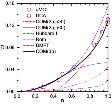
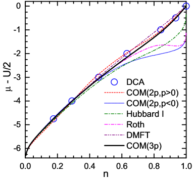
Figure 1: Double occupancy $D$ (left) and scaled chemical potential $\mu-\nicefrac{{U}}{{2}}$ (right) as functions of the filling $n$ for $U=4$ and $T=\nicefrac{{1}}{{6}}$ for COM(3p) (black lines), COM(2p,$p>0$) (dashed red line), COM(2p,$p<0$) (dotted blue line), Hubbard I (dot-dashed green line), Roth (dot-dot-dashed magenta line) and DMFT Capone (dash-dotted purple line). Analytical results are compared with $12\times 12$-site qMC Moreo et al. (1990) and $2$-site DCA Sangiovanni numerical data (red and blue hollow circles, respectively).

In Fig. 1, we report the behavior of the double occupancy $D$ (left panel) and of the scaled chemical potential $\mu-\nicefrac{{U}}{{2}}$ (right panel) as functions of the filling $n$ for $U=4$ and $T=\nicefrac{{1}}{{6}}$. It is evident the very good agreement in the whole range of filling $n$ between COM(3p) and the $12\times 12$-site qMC Moreo et al. (1990) and $2$-site DCA Sangiovanni numerical data. The double occupancy $D$ features a very elaborated behavior presenting a continuos, but well defined, change of slope on approaching half filling. COM(3p) correctly catches this feature, while all other presented solutions do not manage to achieve the same level of agreement over the whole range of filling. Hubbard I and Roth solutions report values of the $D$ extremely far from the numerical ones and always much smaller than these latter, showing a tendency to an excess of correlations present in such solutions. DMFT Capone performs extremely well, with respect to numerical data, at low-intermediate values of filling, but at intermediate-high ones features values of $D$ larger than the numerical ones. This is a clear evidence of a lack of correlations for this value of $U$. COM(2p, $p<0$) performs really very well too at low-intermediate values of filling, but on increasing $U$ it shows an excess of correlations close to half filling (it is actually insulating for any finite value of $U$ at half filling). In COM(2p, $p>0$), it is evident a complete suppression of $D$ at low values of the filling as well as a small, but visible, discrepancy in the slope close to half filling. COM(3p) evidently has the capability to correctly interpolate between the two COM(2p) solutions sticking to COM(2p, $p<0$) at low-intermediate values of filling and even improving on COM(2p, $p>0$) at intermediate-high values of filling. The DCA data for the chemical potential show a concavity in proximity of half filling that is correctly caught by COM(3p) and COM(2p, $p>0$) and not by COM(2p, $p<0$), Hubbard I and Roth solutions. Roth solution actually reports a rather evident region of thermodynamic instability, $\frac{d\mu}{dn}<0$, close to half filling. As a matter of fact, $U=4$ induces already quite strong electronic correlations: the chemical potential gets ready to open a gap for higher values of $U$ and $n=1$. COM(2p, $p<0$), Hubbard I and Roth solutions place themselves always on the strongly correlated side and report values of $\mu$ quite far from the numerical ones: their particle counting - actual effective filling - is definitely far from the exact one. DMFT Capone solution does not catch the correct concavity again showing a lack of correlations for this value of $U$, but it features values of $\mu$ very close to the numerical ones in the whole range of filling $n$ although not so close as COM(3p) ones in proximity of half-filling, which is the most interesting region.

III.2 Quasi-particle energy dispersions: solution characterization

In Fig. 2, we report the energy bands $E_{m}\left(\mathbf{k}\right)$ along the principal directions of the first Brillouin zone ($\Gamma=(0,0)$ $\to$ $S=(\nicefrac{{\pi}}{{2}},\nicefrac{{\pi}}{{2}})$ $\to$ $M=(\pi,\pi)$ $\to$ $X=(\pi,0)$ $\to$ $Y=(0,\pi)$ $\to$ $\Gamma=(0,0)$) at $T=\nicefrac{{1}}{{6}}$, $U=4$ and two different values of the filling $n=0.2$ (left panel) and $n=0.9$ (right panel). At $n=0.2$, it is evident that the occupied bands are almost identical across all reported COM solutions. Actually, COM(3p) is characterized by a small, but finite, occupation of its LHB, besides the occupation of its central band (CB), which is the band coinciding with the COM(2p) LHBs. This can be understood in terms of the proximity of COM(3p) LHB to the chemical potential at the $M$ point. LHB is the only occupied band in COM(2p,$p<0$) at all finite values of $U$. At $n=0.9$, the occupied region in energy-momentum space across the three COM solutions is instead quite different, although some similarities can still be found. In particular, as regards the regions close to the chemical potential at the $\Gamma$ point and along the main anti-diagonal (the $X-Y$ line). COM(3p) CB, which was the main actor at low fillings, tends to systematically lose occupation in favor of the LHB. Close to half filling, this latter eventually exceeds the former in occupation and collects more and more of it on increasing $U$ while the CB depletes on approaching the metal-insulator transition. As regards COM(2p,$p>0$) instead, UHB plays a minor role all the way up to the metal-insulator transition. It collects a small fraction of the electronic occupation and only above a certain intermediate value of the filling. It is evident that COM(3p) CB is still almost pinned to the chemical potential along the main anti-diagonal (the $X-Y$ line); the van Hove singularity lies little below the Fermi level. Accordingly, changing the filling in this region of low doping (from $n=0.85$ to $n=1$) has mainly the effect to induce a transfer of spectral weight between the bands and between their components in terms of fields of the basis, as one would expect in a strongly correlated regime, rather than shifting the chemical potential more or less rigidly within the bands, as it could be expected at small fillings and weak interactions. It is also evident that the LHB has still a minor role with respect to the CB, which collects the vast majority of the occupied states. It is worth noting that the spin-spin correlations are already present, but not yet so strong to determine the reduction of the bandwidth in the energy-momentum space region shared by CB and LHB. It is worth noticing that COM(3p) bands are quite close to COM(2p,$p<0$) ones.

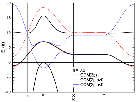
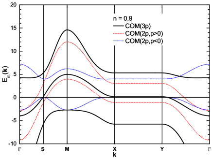
Figure 2: Energy bands $E_{m}\left(\mathbf{k}\right)$ along the principal directions of the first Brillouin zone ($\Gamma=(0,0)$ $\to$ $S=(\nicefrac{{\pi}}{{2}},\nicefrac{{\pi}}{{2}})$ $\to$ $M=(\pi,\pi)$ $\to$ $X=(\pi,0)$ $\to$ $Y=(0,\pi)$ $\to$ $\Gamma=(0,0)$) at $T=\nicefrac{{1}}{{6}}$, $U=4$ and two different values of the filling $n=0.2$ (left) and $n=0.9$ (right) for COM(3p) (black line), COM(2p,$p>0$) (red line) and COM(2p,$p<0$) (blue line).

III.3 Momentum resolved quantities

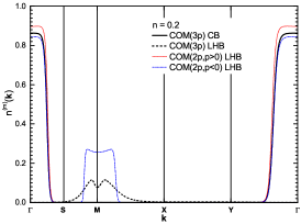
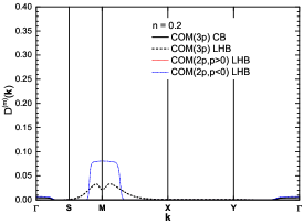
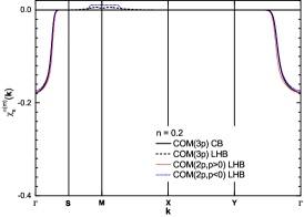
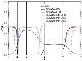
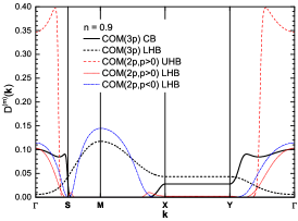
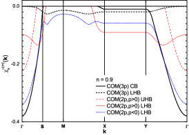
Figure 3: Momentum-distribution function per band and spin $n^{\left(m\right)}\left(\mathbf{k}\right)$ (left), double-occupancy components per band $D^{\left(m\right)}\left(\mathbf{k}\right)$ (center) and nearest-neighbor spin correlation function components per band $\chi_{s}^{\alpha\left(m\right)}\left(\mathbf{k}\right)$ (right) along the principal directions of the first Brillouin zone ($\Gamma=(0,0)$ $\to$ $S=(\nicefrac{{\pi}}{{2}},\nicefrac{{\pi}}{{2}})$ $\to$ $M=(\pi,\pi)$ $\to$ $X=(\pi,0)$ $\to$ $Y=(0,\pi)$ $\to$ $\Gamma=(0,0)$) at $T=\nicefrac{{1}}{{6}}$, $U=4$ and two different values of the filling $n=0.2$ (top) and $n=0.9$ (bottom) for COM(3p) (solid and short-dashed black line), COM(2p,$p>0$) (dashed and short-dotted red line) and COM(2p,$p<0$) (short-dash-dotted blue line).

Given the decomposition of the momentum-dependent correlation functions per band reported in Eqs. 18 and 19, it is possible to define a similar decomposition for any quantity that can be expressed in terms of correlation functions of the chosen operatorial basis, that is for any quantity computable within the reported approximation. In particular, we have the following expressions for the filling $n$, the double occupancy $D$ and the nearest-neighbor spin correlation function $\chi_{s}^{\alpha}$

$$n =2\sum\limits_{m=1}^{3}\frac{1}{N}\sum_{\mathbf{k}}n^{\left(m\right)}\left(\mathbf{k}\right)$$ (44)

$$D =\sum\limits_{m=1}^{3}\frac{1}{N}\sum_{\mathbf{k}}D^{\left(m\right)}\left(\mathbf{k}\right)$$ (45)

$$\chi_{s}^{\alpha} =\sum\limits_{m=1}^{3}\frac{1}{N}\sum_{\mathbf{k}}\chi_{s}^{\alpha\left(m\right)}\left(\mathbf{k}\right)$$ (46)

where

$$n^{\left(m\right)}\left(\mathbf{k}\right) =\frac{1}{2}f_{\mathrm{F}}\left(E_{m}\left(\mathbf{k}\right)\right)\sigma_{cc}^{\left(m\right)}\left(\mathbf{k}\right)$$ (47)

$$D^{\left(m\right)}\left(\mathbf{k}\right) =f_{\mathrm{F}}\left(E_{m}\left(\mathbf{k}\right)\right)\sigma_{22}^{\left(m\right)}\left(\mathbf{k}\right)$$ (48)

$$\chi_{s}^{\alpha\left(m\right)}\left(\mathbf{k}\right) =\frac{2\alpha\left(\mathbf{k}\right)f_{\mathrm{F}}\left(E_{m}\left(\mathbf{k}\right)\right)}{2I_{11}I_{22}-C_{\eta\eta}}\times$$

$$\times\left(I_{11}C_{c\eta}^{\alpha}\sigma_{2c}^{\left(m\right)}\left(\mathbf{k}\right)+I_{22}C_{c\xi}^{\alpha}\sigma_{1c}^{\left(m\right)}\left(\mathbf{k}\right)\right)$$ (49)

In Fig. 3, we report the momentum-distribution function per band and spin $n^{\left(m\right)}\left(\mathbf{k}\right)$ (left column), the double-occupancy components per band $D^{\left(m\right)}\left(\mathbf{k}\right)$ (center column) and the nearest-neighbor spin correlation function components per band $\chi_{s}^{\alpha\left(m\right)}\left(\mathbf{k}\right)$ (right column) along the principal directions of the first Brillouin zone ($\Gamma=(0,0)$ $\to$ $S=(\nicefrac{{\pi}}{{2}},\nicefrac{{\pi}}{{2}})$ $\to$ $M=(\pi,\pi)$ $\to$ $X=(\pi,0)$ $\to$ $Y=(0,\pi)$ $\to$ $\Gamma=(0,0)$) at $T=\nicefrac{{1}}{{6}}$, $U=4$ and two different values of the filling $n=0.2$ (top row) and $n=0.9$ (bottom row). Components from not reported bands are zero or definitely negligible.

At $n=0.2$, $n^{\left(m\right)}\left(\mathbf{k}\right)=\frac{1}{2}\mathcal{F}_{\mathbf{k}}\left[\left\langle c^{\dagger}(\mathbf{i})\cdot c(\mathbf{j}\right\rangle)\right]_{m}$ shows that reported COM bands have a similar and quite ordinary occupations except for the region close to $M$ that is occupied only for COM(3p) and COM(2p,$p<0$) LHBs. This is the result of the peculiar shape of such bands (see Fig. 2) that closely recalls the bending driven by antiferromagnetic fluctuations and the simultaneous occupation of $\Gamma$ and $M$ points. What is really surprising is the fact that the major, almost the only, contribution to the double occupancy ($D^{\left(m\right)}\left(\mathbf{k}\right)=\frac{1}{2}\mathcal{F}_{\mathbf{k}}\left[\left\langle\eta^{\dagger}(\mathbf{i})\cdot\eta(\mathbf{j}\right\rangle)\right]_{m}$) comes just from the this last region in momentum (close to $M$ point). This is really counterintuitive as one expects those branches of energy-momentum dispersion to have such a shape because of the strong antiferromagnetic fluctuations and to be the main seat of electrons contributing to single occupation and, therefore, with well-formed spin momenta. As a matter of fact, the contribution to $D^{\left(m\right)}\left(\mathbf{k}\right)$ close to $M$ should be correctly read as the main (actually the only) contribution to the kinetic energy coming from the $\eta$ Hubbard operators, that is from those electrons moving between double occupied sites. In fact, this situation well explains the almost identical value of the double occupancy for COM(3p) and COM(2p,$p<0$) at this filling, where the motion between doubly occupied sites is allowed, as well as the almost negligible value for COM(2p,$p>0$), where the motion between doubly occupied sites is definitely negligible as it is confined to the UHB, which is empty for this value of the filling. The decomposition of $\chi_{s}^{\alpha\left(m\right)}\left(\mathbf{k}\right)$ shows the expected negative contribution by the electrons close to $\Gamma$ point and an almost negligible positive contribution by those close to $M$ point. At such low value of the filling, we can expect very weak spin correlations and the contribution close to $\Gamma$ point is not so large as well as the whole momentum dependence very little structured.

At $n=0.9$, $n^{\left(m\right)}\left(\mathbf{k}\right)$ shows how much COM bands differ in occupation between the three reported solutions for a value of the filling where quite intense correlations are expected. COM(3p) features an occupation of the CB close to $\Gamma$ point quite reduced with respect to that sported at $n=0.2$, even if we take into account that it is now spanning a quite larger region in momentum and the main anti-diagonal (the $X-Y$ line) is somewhat filled too. This can be explained by noting that the LHB, which at $n=0.2$ was filled only close to $M$ point, features now a quite relevant occupation spanning all over the first Brillouin zone and, in particular, at the $M$ point and along the main anti-diagonal (the $X-Y$ line). Accordingly, we expect the physics of COM(3p) solution to be determined by both bands at the same time and on almost equal footing. Overall, COM(2p,$p<0$) occupation is very similar to the COM(3p) one although concentrated in the only occupied band, the LHB. As a matter of fact, COM(2p,$p<0$) LHB seems to interpolate between the LHB and the CB of COM(3p) showing once more the very strict connections between these two solutions. COM(2p,$p>0$) features instead similar occupations for the two bands except for the extension towards the main anti-diagonal (the $X-Y$ line) of the almost completely filled LHB. The region in momentum close to $M$ remains anyhow empty marking the greatest difference to the other two solutions. Coming to $D^{\left(m\right)}\left(\mathbf{k}\right)$, COM(3p) solution features again a complementary presence between CB and LHB with the exception of the main anti-diagonal (the $X-Y$ line) where the more marked difference reported for $n^{\left(m\right)}\left(\mathbf{k}\right)$ is greatly reduced. Bare looking at the values of $D^{\left(m\right)}\left(\mathbf{k}\right)$ reported along these principal direction, COM(2p,$p<0$) should have an overall value of $D$ quite similar to that of COM(3p), but this is quite not right and can be explained by looking at the region in momentum along the main anti-diagonal (the $X-Y$ line) and close to it (even along the main diagonal: the $\Gamma-M$ line). Although, COM(2p,$p<0$) LHB is lying over the chemical potential in this region of momentum, the double occupancy contribution is definitely negligible marking a huge difference to the CB of COM(3p) that occupies the same region in momentum-frequency space. This is one of the net improvements of the COM(3p) solution over COM(2p,$p<0$) one; an improvement that reflects in many other physical quantities. COM(2p,$p>0$) contributions come both (for LHB and UHB) from the region in momentum close to $\Gamma$ clearly showing that although the overall value of $D$ is quite similar, clearly by accident, between COM(3p) and COM(2p,$p>0$), its physical origin, in terms of quasi-particle contributions and of their momentum-frequency dispersions, is very different and explains the quite different behavior in terms of slope of $D$ as a function of the filling $n$. Let us come to $\chi_{s}^{\alpha\left(m\right)}\left(\mathbf{k}\right)$. As regards COM(3p), the CB brings a much larger contribution, with respect to $n=0.2$, that extends along the main anti-diagonal (the $X-Y$ line). LHB contribution is much smaller, but definitely larger than at $n=0.2$ and negative. Accordingly, it is just the CB, which originates from the third basic field describing the nearest-neighbor antiferromagnetic fluctuations, to bring the larger contribution as one would have expected. Therefore, having such a field in the basis results as one of the main ingredients in order to get such a good performance in comparing this solution with numerical ones Avella (2014). COM(2p,$p<0$) contributions to $\chi_{s}^{\alpha\left(m\right)}\left(\mathbf{k}\right)$ all come from the only occupied band, the LHB, and once more seem to mime the overall behavior of COM(3p). COM(2p,$p>0$) has a completely different behavior. In particular, the contribution of the LHB close to the $\Gamma$ point is quite difficult to understand: instead of increasing in absolute value towards the $\Gamma$ point, it decreases leading to the presence of a maximum absolute value for a value of momentum that coincide with the Fermi surface of the related COM(2p,$p>0$) UHB.

IV Summary

In this manuscript, we have first recollected the main analytical expressions defining a recently proposed, within the framework of the Composite Operator MethodThe ; Avella and Mancini (2012b), three-pole solution for the two-dimensional Hubbard model Avella (2014). Together with the two Hubbard fields, well describing the physics at the energy scale of $U$, the presence of a third field, embedding the strong antiferromagnetic fluctuations, has enormously boosted the performance of COM(3p) solution with respect to COM(2p) ones. The extremely positive comparison with the data obtained by different numerical methods for momentum-integrated quantities (e.g. local properties) as functions of all model parameters (filling, on-site Coulomb repulsion and temperature) as well as for the energy bands of the system Avella (2014) makes this solution extremely interesting to be analyzed further. Here, we have reported a summary of the behavior of the basic local quantities - the double occupancy and the chemical potential -, together with the quasi-particle energy dispersions definitely necessary to guide the subsequent analysis, which is the main focus of the present manuscript: the study of the momentum-resolved components of filling (i.e. the momentum distribution function), double occupancy and nearest-neighbor spin correlation function. The analysis has been extended to COM(2p) solutions that have been used as primary reference as in the main paper Avella (2014). Analyzing the momentum-resolved quantities, it emerges very clearly the role played by the third field with respect to the two Hubbard ones in determining the behavior of many relevant quantities and allowing to get the extremely good comparison with numerical results. In particular, the proximity between COM(3p) and COM(2p,$p<0$) solutions is further reinforced and better understood giving a guideline to further improve and, possibly, optimize the application of the COM to the Hubbard model with the choice of a fourth field solving the few remaining issues with COM(3p)Avella (2014).