Composite Operator Method analysis of the underdoped cuprates puzzle

Abstract

The microscopical analysis of the unconventional and puzzling physics of the underdoped cuprates, as carried out lately by means of the Composite Operator Method (COM) applied to the two-dimensional (2D) Hubbard model, is reviewed and systematized. The 2D Hubbard model has been adopted as, since the very early days of unconventional high-$T_{c}$ superconductivity, it has been considered the minimal model capable to describe the most peculiar features of cuprates held responsible for their anomalous behavior. As a matter of fact, understanding the physics of the 2D Hubbard model itself constitutes one of the most intriguing challenges in condensed matter theory. In the last fifteen years, COM has proved to be a quite powerful non-perturbative, fully-analytical, self-consistent, microscopical approximation methods specifically devised to deal with strongly correlated systems (SCSs). COM is designed to endorse, since its foundations, the systematic emergence in any SCS of new elementary excitations described by composite operators obeying non-canonical algebras. COM is formulated to deal with the unusual features of such composite operators and compute the unconventional properties of SCSs. In this case (underdoped cuprates – 2D Hubbard model), the residual interactions – beyond a $2$-pole approximation – between the new elementary electronic excitations, dictated by the strong local Coulomb repulsion and well described by the two Hubbard composite operators, have been treated within the Non Crossing Approximation (NCA). The two-particle spin and charge propagators, appearing in the electronic self-energy thanks to the composite nature of the new elementary electronic excitations, have been computed fully-microscopically within the very same framework, just neglecting any explicit damping in a first approximation. Given this recipe and exploiting the few unknowns to enforce the Pauli principle content in the solution, it is possible to qualitatively describe – finite and specific longer-distance hopping terms are needed for a quantitative comparison to a specific material – some of the anomalous features of high-T_c cuprate superconductors such as large vs. small Fermi surface dichotomy, Fermi surface deconstruction (appearance of Fermi arcs), nodal vs. anti-nodal physics, pseudogap(s), kinks in the electronic dispersion. The resulting scenario envisages a smooth crossover between an ordinary weakly-interacting metal sustaining weak, short-range antiferromagnetic correlations in the overdoped regime to an unconventional poor metal characterized by very strong, long-but-finite-range antiferromagnetic correlations leading to momentum-selective non-Fermi liquid features as well as to the opening of a pseudogap and to the striking differences between the nodal and the anti-nodal dynamics in the underdoped regime.

I Introduction

I.1 Composite fields

One of the most intriguing challenges in modern condensed matter physics is the theoretical description of the anomalous behaviors experimentally observed in many novel materials. By anomalous behaviors we mean those not predicted by standard many-body theory; that is, behaviors in contradiction with the Fermi-liquid framework and diagrammatic expansions. The most relevant characteristic of such novel materials is the presence of so strong correlations among the electrons that classical schemes based on the band picture and the perturbation theory are definitely inapplicable. Accordingly, it is necessary to move from a single-electron physics to a many-electron physics, where the dominant contributions come from the strong interactions among the electrons: usual schemes are simply inadequate and new concepts must be introduced.

The classical techniques are based on the hypothesis that the interactions among the electrons are weak enough, or sufficiently well screened, to be properly taken into account within the framework of perturbative/diagrammatic methods. However, as many and many experimental and theoretical studies of highly correlated systems have shown, with more and more convincing evidence, all these methods are no more viable. The main concept that breaks down is the existence of the electrons as particles or quasi-particles with quite-well-defined properties. The presence of the interactions radically modifies the properties of the particles and, at a macroscopic level, what are observed are new particles (actually they are the only observable ones) with new peculiar properties entirely determined by the dynamics and by the boundary conditions (i.e. the phase under study, the external fields, …). These new objects appear as the final result of the modifications imposed by the interactions on the original particles and contain, by the very beginning, the effects of correlations.

On the basis of this evidence, one is induced to move the attention from the original fields to the new fields generated by the interactions. The operators describing these excitations, once they have been identified, can be written in terms of the original ones and are known as composite operators. The necessity of developing a formulation to treat composite operators as fundamental objects of the many-body problem in condensed matter physics has been deeply understood and systematically noticed since quite long time. Recent years have seen remarkable achievements in the development of a modern many-body theory in solid-state physics in the form of an assortment of techniques that may be termed composite particle methods. The foundations of these types of techniques may be traced back to the work of Bogoliubov Bogoliubov (1947) and later to that of Dancoff Dancoff (1950). The work of Zwanzig Zwanzig (1961), Mori Mori (1965); Plakida et al. (1995, 2003); Plakida and Oudovenko (2007); Adam and Adam (2007); Plakida (2010) and Umezawa Umezawa (1993) definitely deserves to be mentioned too. Closely related to this work is that of Hubbard Hubbard (1963, 1964a, 1964b), Rowe Rowe (1968), Roth Roth (1969) and Tserkovnikov Tserkovnikov (1981a, b). The slave boson method Barnes (1976); Coleman (1984); Kotliar and Ruckenstein (1986), the spectral density approach Kalashnikov and Fradkin (1969); Nolting (1972), the diagram technique for Hubbard operators Izyumov and Yu.N. (1989), the cumulant expansion based diagram technique Moskalenko and Vladimir (1990), the generalized tight-binding method Ovchinnikov and Val’kov (2004); Korshunov et al. (2005); Ovchinnikov et al. (2006), self-consistent projection operator method Kakehashi and Fulde (2004, 2005), operator projection method Onoda and Imada (2001a, b, 2003) and the composite operator method (COM) The ; Avella and Mancini (2012) are along the same lines. This large class of theories is very promising as it is based on the firm conviction that strong interactions call for an analysis in terms of new elementary fields embedding the greatest possible part of the correlations so permitting to overcome the problem of finding an appropriate expansion parameter. However, one price must be paid. In general, composite fields are neither Fermi nor Bose operators, since they do not satisfy canonical (anti)commutation relations, and their properties must be determined self-consistently. They can only be recognized as fermionic or bosonic operators according to the number and type of the constituting original particles. Accordingly, new techniques have to be developed in order to deal with such composite fields and to design diagrammatic schemes where the building blocks are the propagators of such composite fields: standard diagrammatic expansions and the Wick’s theorem are no more valid. The formulation of the Green’s function method itself must be revisited and new frameworks of calculations have to be devised.

Following these ideas, we have been developing a systematic approach, the composite operator method (COM) The ; Avella and Mancini (2012), to study highly correlated systems. The formalism is based on two main ideas: (i) use of propagators of relevant composite operators as building blocks for any subsequent approximate calculations; (ii) use of algebra constraints to fix the representation of the relevant propagators in order to properly preserve algebraic and symmetry properties; these constraints will also determine the unknown parameters appearing in the formulation due to the non-canonical algebra satisfied by the composite operators. In the last fifteen years, COM has been applied to several models and materials: Hubbard Hub ; Avella et al. (2004); Krivenko et al. (2005); Odashima et al. (2005); Avella (2014), $p$-$d$ p-d , $t$-$J$ Avella et al. (2002), $t$-$t^{\prime}$-$U$ ttU , extended Hubbard ($t$-$U$-$V$) tUV , Kondo Villani et al. (2000), Anderson And , two-orbital Hubbard 2or ; Plekhanov et al. (2011), Ising Isi , $J_{1}-J_{2}$ Bak et al. (2003); J1J ; Avella et al. (2008), Hubbard-Kondo Avella and Mancini (2006), Cuprates Cup ; Avella and Mancini (2007a, b, 2008, 2009), etc.

I.2 Underdoped cuprates

Cuprate superconductors Bednorz and Müller (1986) display a full range of anomalous features, mainly appearing in the underdoped region, in almost all experimentally measurable physical properties Timusk and Statt (1999); Orenstein and Millis (2000); Damascelli et al. (2003); Eschrig (2006); Sebastian et al. (2012a). According to this, their microscopic description is still an open problem: non-Fermi-liquid response, quantum criticality, pseudogap formation, ill-defined Fermi surface, kinks in the electronic dispersion, etc. remain still unexplained (or at least controversially debated) anomalous features Lee et al. (2006); Tremblay et al. (2006); Sebastian et al. (2012a). In the last years, the attention of the community has been focusing on three main experimental facts Sebastian et al. (2012a): the dramatic change in shape and nature of the Fermi surface between underdoped and overdoped regimes, the appearance of a psedudogap in the underdoped regime, and the striking differentiation between the physics at the nodes and at the anti-nodes in the pseudogap regime. The topological transition of the Fermi surface has been first detected by means of ARPES Damascelli et al. (2003) and reflects the noteworthy differences between the quite-ordinary, large Fermi surface measured in the overdoped regime Hussey et al. (2003); Plate et al. (2005); Peets et al. (2007) and quite well described by LDA calculations Andersen et al. (1995) and quantum oscillations measurements Vignolle et al. (2008), and the ill-defined Fermi arcs appearing in the underdoped regime Shen et al. (2005); Valla et al. (2006); Lee et al. (2006); Kanigel et al. (2006); Hossain et al. (2008); Meng et al. (2009); King et al. (2011). The enormous relevance of these experimental findings, not only for the microscopic comprehension of the high-$T_{c}$ superconductivity phenomenology, but also for the drafting of a general microscopic theory for strongly correlated materials, called for many more measurements in order to explore all possible aspects of such extremely anomalous and peculiar behavior: plenty of quantum oscillations measurements in the underdoped regime Doiron-Leyraud et al. (2007); LeBoeuf et al. (2007); Yelland et al. (2008); Bangura et al. (2008); Sebastian et al. (2008); Audouard et al. (2009); Sebastian et al. (2010a, b, c); Singleton et al. (2010); Vishik et al. (2010); Anzai et al. (2010); Ramshaw et al. (2011); Sebastian et al. (2011a, b, c); Riggs et al. (2011); Laliberte et al. (2011); Vignolle et al. (2011); Sebastian et al. (2012b), Hall effect measurements LeBoeuf et al. (2007), Seebeck effect measurements Laliberte et al. (2011), and heat capacity measurements Riggs et al. (2011). The presence of a quite strong depletion in the electronic density of states, known as pseudogap Norman et al. (2005), is well established thanks to ARPES Damascelli et al. (2003), NMR Alloul et al. (1989), optical conductivity Basov et al. (1999) and quantum oscillations Tranquada et al. (2010) measurements. The microscopic origin of such a loss of single-particle electronic states is still unclear and the number of possible theoretical, as well as phenomenological, explanations has grown quite large in the last few years. As a matter of fact, this phenomenon affects any measurable properties and, accordingly, was the first to be detected in the underdoped regime granting to this latter the first evidences of its exceptionality with respect to the other regimes in the phase diagram. The plethora of theoretical scenarios present in the literature Kivelson et al. (2003); Lee et al. (2006); Carrington and Yelland (2007); Sushkov (2011), tentatively explaining few, some or many of the anomalous features reported by the experiments on underdoped cuprates, can be coarsely divided between those not relying on any translational symmetry breaking Alexandrov and Bratkovsky (1996); Yang et al. (2006); Melikyan and Vafek (2008); Varma (2009); Wilson (2009); Pereg-Barnea et al. (2010) and those instead proposing that it should be some kind of charge and/or spin arrangements to be held responsible for the whole range of anomalous features. Among these latter theories, there are those focusing on the physics at the anti-nodal region and those focusing on the nodal region. We can account for proposals of (as regards the anti-node): a collinear spin AF order Millis and Norman (2007), an AF quantum critical point Haug et al. (2010); Baledent et al. (2011), a 1D charge stripe order Millis and Norman (2007); Harrison and Sebastian (2011) with the addition of a smectic phase Yao et al. (2011). Instead, at the node, we have: a $d$-density wave Chakravarty and Kee (2008), a more-or-less ordinary AF spin order Chubukov and Morr (1997); Avella and Mancini (2007a, b); Avella et al. (2007); Avella and Mancini (2007c); Chen et al. (2008); Avella and Mancini (2008, 2009); Oh et al. (2011), a nodal pocket from bilayer low-$Q$ charge order, slowly fluctuacting Li et al. (2006); Harrison (2011); Harrison and Sebastian (2011, 2012). This latter proposal, which is among the newest on the table, relies on many experimental measurements: STM Edwards et al. (1994); Hoffman et al. (2002); Hanaguri et al. (2004); McElroy et al. (2005); Maki et al. (2005), Neutron scattering Tranquada et al. (2010), X-ray diffraction Liu et al. (2008), NMR Wu et al. (2011), RXS Ghiringhelli et al. (2012), phonon softening Mook et al. (1996); Mook and F. (1999); Reznik et al. (2008). A proposal regarding the emergence of a hidden Fermi liquid Anderson and Casey (2009) is also worth mentioning.

I.3 2D Hubbard Model – Approximation Methods

Since the very beginning Anderson (1987), the two-dimensional Hubbard model Hubbard (1963) has been universally recognized as the minimal model capable to describe the $Cu-O_{2}$ planes of cuprates superconductors. It certainly contains many of the key ingredients by construction: strong electronic correlations, competition between localization and itineracy, Mott physics, and low-energy spin excitations. Unfortunately, although fundamental for benchmarking and fine tuning analytical theories, numerical approaches Bulut (2002) cannot be of help to solve the puzzle of underdoped cuprates owing to their limited resolution in frequency and momentum. On the other hand, there are not so many analytical approaches capable to deal with the quite complex aspects of underdoped cuprates phenomenology Plakida (2010). Among others, the Two-Particle Self-Consistent (TPSC) approach Vilk and Tremblay (1995); Tremblay et al. (2006) has been the first completely microscopic approach to obtain results comparable with the experimental findings. Almost all other promising approaches available in the literature can be essentially divided into two classes. One class makes use of phenomenological expressions for the electronic self-energy and the electronic spin susceptibility Plakida et al. (1995, 2003); Chubukov and Norman (2004); Prelovšek and Ramšak (2005); Plakida and Oudovenko (2007); Adam and Adam (2007); Plakida (2010). The electronic self-energy is usually computed as the convolution of the electronic propagator and of the electronic spin susceptibility. Then, the electronic spin susceptibility is modeled phenomenologically parameterizing correlation length and damping as functions of doping and temperature according to the common belief that the electronic spin susceptibility should present a well developed mode at $M=(\pi,\pi)$ with a damping of Landau type. The DMFT$+\Sigma$ approach Sadovskii (2001); Sadovskii et al. (2005); Kuchinskii et al. (2005, 2006, 2007) also belongs to this class. All cluster-dynamical-mean-field-like theories (cluster-DMFT theories) Maier et al. (2005); Tremblay et al. (2006); Stanescu et al. (2006) (the cellular dynamical mean-field theory (C-DMFT) Kotliar et al. (2001); Haule and Kotliar (2007), the dynamical cluster approximation (DCA) Hettler et al. (1998) and the cluster perturbation theory (CPT) Sénéchal et al. (2000); Sénéchal and Tremblay (2004); Tremblay et al. (2006)) belong to the second class. The dynamical Mean-Field Theory (DMFT) Georges et al. (1996); Kotliar and D. (2004); Kotliar et al. (2006); Held (2007); Izyumov and V.I. (2008) cannot tackle the underdoped cuprates puzzle because its self-energy has the same identical value at each point on the Fermi surface without any possible differentiation between nodal and antinodal physics or visible and phantom portion of the Fermi surface. The cluster-DMFT theories instead can, in principle, deal with both coherent quasi-particles and marginal ones within the same Fermi surface. These theories usually self-consistently map the generic Hubbard problem to a few-site lattice Anderson problem and solve this latter by means of, mainly, numerical techniques. What really distinguishes one formulation from another, within this second class, is the procedure used to map the small cluster on the infinite lattice. Anyway, it is worth noticing that these approaches often relies on numerical methods in order to close their self-consistency cycles (with the above mentioned limitations in frequency and momentum resolutions and with the obvious difficulties in the physical interpretation of their results) and always face the emergence of a quite serious periodization problem since a cluster embedded in the lattice violates its periodicity. The Composite Operator Method (COM) The ; Avella and Mancini (2012) does not belong to any of these two classes of theoretical formulations and has the advantage to be completely microscopic, exclusively analytical, and fully self-consistent. COM recipe uses three main ingredients The ; Avella and Mancini (2012): composite operators, algebra constraints, and residual self-energy treatment. Composite operators are products of electronic operators and describe the new elementary excitations appearing in the system owing to strong correlations. According to the system under analysis The ; Avella and Mancini (2012), one has to choose a set of composite operators as operatorial basis and rewrite the electronic operators and the electronic Green’s function in terms of this basis. One should think of composite operators just as a more convenient starting point, with respect to electronic operators, for any mean-field-like approximation/perturbation scheme. Algebra constraints are relations among correlation functions dictated by the non-canonical operatorial algebra closed by the chosen operatorial basis The ; Avella and Mancini (2012). Other ways to obtain algebra constraints rely on the symmetries enjoined by the Hamiltonian under study, the Ward-Takahashi identities, the hydrodynamics, etc The ; Avella and Mancini (2012). One should think of algebra constraints as a way to restrict the Fock space on which the chosen operatorial basis acts to the Fock space of physical electrons. Algebra constraints are used to compute unknown correlation functions appearing in the calculations. Interactions among the elements of the chosen operatorial basis are described by the residual self-energy, that is, the propagator of the residual term of the current after this latter has been projected on the chosen operatorial basis The ; Avella and Mancini (2012). According to the physical properties under analysis and the range of temperatures, dopings, and interactions you want to explore, one has to choose an approximation to compute the residual self-energy. In the last years, we have been using the $n-$pole Approximation Hub ; Odashima et al. (2005); p-d ; Avella et al. (2002); ttU ; tUV ; 2or ; Plekhanov et al. (2011); Isi ; Avella and Mancini (2006); Cup , the Asymptotic Field Approach Villani et al. (2000); And , the NCA Avella (2003); Avella et al. (2004); Krivenko et al. (2005); Avella and Mancini (2007a, b, 2008, 2009) and the Two-Site Resolvent Approach Matsumoto et al. (1996); Matsumoto and Mancini (1997). You should think of the residual self-energy as a measure in the frequency and momentum space of how much well defined are, as quasi-particles, your composite operators. It is really worth noticing that, although the description of some of the anomalous features of underdoped cuprates given by COM qualitatively coincide with those obtained by TPSC Tremblay et al. (2006) and by the two classes of formulations mentioned above, the results obtained by means of COM greatly differs from those obtained within the other methods as regards the evolution with doping of the dispersion and of the Fermi surface and, at the moment, no experimental result can tell which is the unique and distinctive choice nature made.

I.4 Outline

To study the underdoped cuprates modeled by the 2D Hubbard model (see Sec. II.1), we start from a basis of two composite operators (the two Hubbard operators) and formulate the Dyson equation (see Sec. II.2) in terms of the $2$-pole approximated Green’s function (see Sec. II.3). According to this, the self-energy is the propagator of non-local composite operators describing the electronic field dressed by charge, spin, and pair fluctuations on the nearest-neighbor sites. Then, within the Non-Crossing Approximation (NCA) Bosse et al. (1978), we obtain a microscopic self-energy written in terms of the convolution of the electronic propagator and of the charge, spin, and pair susceptibilities (see Sec. II.4). Finally, we close, fully analytically, the self-consistency cycle for the electronic propagator by computing microscopic susceptibilities within a $2$-pole approximation (see Sec. II.5). Our results (see Sec. II.4) show that, within COM, the two-dimensional Hubbard model can describe some of the anomalous features experimentally observed in underdoped cuprates phenomenology. In particular, we show how Fermi arcs can develop out of a large Fermi surface (see Sec. III.2), how pseudogap can show itself in the dispersion (see Sec. III.1) and in the density of states (see Sec. III.3), how non-Fermi liquid features can become apparent in the momentum distribution function (see Sec. III.4) and in the frequency and temperature dependences of the self-energy (see Sec. III.5), how much kinked the dispersion can get on varying doping (see Sec. III.1), and why, or at least how, spin-dynamics can be held responsible for all this (see Sec. III.6). Finally (see Sec. IV), we summarize the current status of the scenario emerging by these theoretical findings and which are the perspectives.

II Framework

II.1 Hamiltonian

The Hamiltonian of the two-dimensional Hubbard model reads as

$$H=\sum_{\mathbf{ij}}\left(-\mu\delta_{\mathbf{ij}}-4t\alpha_{\mathbf{ij}}\right)c^{\dagger}(i)c(j)+U\sum_{\mathbf{i}}n_{\uparrow}(i)n_{\downarrow}(i)$$ (1)

where

$$c(i)=\left(\begin{array}[]{c}c_{\uparrow}(i)\\ c_{\downarrow}(i)\end{array}\right)$$ (2)

is the electron field operator in spinorial notation and Heisenberg picture ($i=(\mathbf{i},t_{i})$), $\mathbf{i}=\mathbf{R_{i}}$ is a vector of the Bravais lattice, $n_{\sigma}(i)=c_{\sigma}^{\dagger}(i)c_{\sigma}(i)$ is the particle density operator for spin $\sigma$, $n(i)=\sum_{\sigma}n_{\sigma}(i)$ is the total particle density operator, $\mu$ is the chemical potential, $t$ is the hopping integral and the energy unit, $U$ is the Coulomb on-site repulsion and $\alpha_{\mathbf{ij}}$ is the projector on the nearest-neighbor sites

$$\alpha_{\mathbf{ij}} = \frac{1}{N}\sum_{\mathbf{k}}\mathrm{e}^{\mathrm{i}\mathbf{k}\cdot(\mathbf{R_{i}}-\mathbf{R_{j}})}\alpha(\mathbf{k})$$

$$\alpha(\mathbf{k}) = \frac{1}{2}\left[\cos(k_{x}a)+\cos(k_{y}a)\right]$$ (3)

where $\mathbf{k}$ runs over the first Brillouin zone, $N$ is the number of sites and $a$ is the lattice constant.

II.2 Green’s functions and Dyson equation

Following COM prescriptions The ; Avella and Mancini (2012), we chose a basic field; in particular, we select the composite doublet field operator

$$\psi(i)=\left(\begin{array}[]{c}\xi(i)\\ \eta(i)\end{array}\right)$$ (4)

where $\eta(i)=n(i)c(i)$ and $\xi(i)=c(i)-\eta(i)$ are the Hubbard operators describing the main subbands. This choice is guided by the hierarchy of the equations of motion and by the fact that $\xi(i)$ and $\eta(i)$ are eigenoperators of the interacting term in the Hamiltonian (1). The field $\psi(i)$ satisfies the Heisenberg equation

$$\mathrm{i}\frac{\partial}{\partial t}\psi(i)=J(i)=\left(\begin{array}[]{c}-\mu\xi(i)-4tc^{\alpha}(i)-4t\pi(i)\\ (U-\mu)\eta(i)+4t\pi(i)\end{array}\right)$$ (5)

where the higher-order composite field $\pi(i)$ is defined by

$$\pi(i)=\frac{1}{2}\sigma^{\mu}n_{\mu}(i)c^{\alpha}(i)+c(i)c^{\dagger\alpha}(i)c(i)$$ (6)

with the following notation: $n_{\mu}(i)=c^{\dagger}(i)\sigma_{\mu}c(i)$ is the particle- ($\mu=0$) and spin- ($\mu=1,\,2,\,3$) density operator, $\sigma_{\mu}=\left(1,\,\vec{\sigma}\right)$, $\sigma^{\mu}=\left(-1,\,\vec{\sigma}\right)$, $\sigma_{k}\,\left(k=1,\,2,\,3\right)$ are the Pauli matrices. Hereafter, for any operator $\Phi(i)$, we use the notation $\Phi^{\alpha}(\mathbf{i},t)=\sum_{\mathbf{j}}\alpha_{\mathbf{ij}}\Phi(\mathbf{j},t)$.

It is always possible to decompose the source $J(i)$ under the form

$$J(i)=\varepsilon(-\mathrm{i}\nabla)\psi(i)+\delta J(i)$$ (7)

where the linear term represents the projection of the source on the basis $\psi(i)$ and is calculated by means of the equation

$$\langle\{\delta J(\mathbf{i},t),\,\psi^{\dagger}(\mathbf{j},t)\}\rangle=0$$ (8)

where $\langle\cdots\rangle$ stands for the thermal average taken in the grand-canonical ensemble.

This constraint assures that the residual current $\delta J(i)$ contains all and only the physics orthogonal to the chosen basis $\psi(i)$. The action of the derivative operator $\varepsilon(-\mathrm{i}\nabla)$ on $\psi(i)$ is defined in momentum space

$$\varepsilon(-\mathrm{i}\nabla)\psi(i) = \varepsilon(-\mathrm{i}\nabla)\frac{1}{\sqrt{N}}\sum_{\mathbf{k}}\mathrm{e}^{\mathrm{i}\mathbf{k}\cdot\mathbf{R_{i}}}\psi(\mathbf{k},t)=\frac{1}{\sqrt{N}}\sum_{\mathbf{k}}\mathrm{e}^{\mathrm{i}\mathbf{k}\cdot\mathbf{R_{i}}}\varepsilon(\mathbf{k})\psi(\mathbf{k},t)$$

where $\varepsilon(\mathbf{k})$ is named energy matrix.

The constraint (8) gives

$$m(\mathbf{k})=\varepsilon(\mathbf{k})I(\mathbf{k})$$ (9)

after defining the normalization matrix

$$I(\mathbf{i,j})=\langle\{\psi(\mathbf{i},t),\,\psi^{\dagger}(\mathbf{j},t)\}\rangle=\frac{1}{N}\sum_{\mathbf{k}}\mathrm{e}^{\mathrm{i}\mathbf{k}\cdot(\mathbf{R_{i}-R_{j}})}I(\mathbf{k})$$ (10)

and the $m$-matrix

$$m(\mathbf{i,j})=\langle\{J(\mathbf{i},t),\,\psi^{\dagger}(\mathbf{j},t)\}\rangle=\frac{1}{N}\sum_{\mathbf{k}}\mathrm{e}^{\mathrm{i}\mathbf{k}\cdot(\mathbf{R_{i}-R_{j}})}m(\mathbf{k})$$ (11)

Since the components of $\psi(i)$ contain composite operators, the normalization matrix $I(\mathbf{k})$ is not the identity matrix and defines the spectral content of the excitations. In fact, the composite operator method has the advantage of describing crossover phenomena as the phenomena in which the weight of some operator is shifted to another one.

By considering the two-time thermodynamic Green’s functions Bogoliubov and Tyablikov (1959); Zubarev (1960, 1974), let us define the retarded function

$$G(i,j)=\langle R[\psi(i)\psi^{\dagger}(j)]\rangle=\theta(t_{i}-t_{j})\langle\{\psi(i),\,\psi^{\dagger}(j)\}\rangle$$ (12)

By means of the Heisenberg equation (5) and using the decomposition (7), the Green’s function $G(i,j)$ satisfies the equation

$$\Lambda(\partial_{i})G(i,j)\Lambda^{\dagger}(\overleftarrow{\partial}_{j})=\Lambda(\partial_{i})G_{0}(i,j)\Lambda^{\dagger}(\overleftarrow{\partial}_{j})+\langle R[\delta J(i)\delta J^{\dagger}(j)]\rangle$$ (13)

where the derivative operator $\Lambda(\partial_{i})$ is defined as

$$\Lambda(\partial_{i})=\mathrm{i}\frac{\partial}{\partial t_{i}}-\varepsilon(-\mathrm{i}\nabla_{i})$$ (14)

and the propagator $G^{0}(i,j)$ is defined by the equation

$$\Lambda(\partial_{i})G^{0}(i,j)=\mathrm{i}\delta(t_{i}-t_{j})I(i,j)$$ (15)

By introducing the Fourier transform

$$G(i,j)=\frac{1}{N}\sum_{\mathbf{k}}\frac{\mathrm{i}}{2\pi}\int d\omega\mathrm{e}^{\mathrm{i}\mathbf{k}\cdot(\mathbf{R_{i}}-\mathbf{R_{j}})-\mathrm{i}\omega(t_{i}-t_{j})}G(\mathbf{k},\omega)$$ (16)

equation (13) in momentum space can be written as

$$G(\mathbf{k},\omega)=G^{0}(\mathbf{k},\omega)+G^{0}(\mathbf{k},\omega)I^{-1}(\mathbf{k})\Sigma(\mathbf{k},\omega)G(\mathbf{k},\omega)$$ (17)

and can be formally solved as

$$G(\mathbf{k},\omega)=\frac{1}{\omega-\varepsilon(\mathbf{k})-\Sigma(\mathbf{k},\omega)}I(\mathbf{k})$$ (18)

where the self-energy $\Sigma(\mathbf{k},\omega)$ has the expression

$$\Sigma(\mathbf{k},\omega)=B_{irr}(\mathbf{k},\omega)I^{-1}(\mathbf{k})$$ (19)

with

$$B(\mathbf{k},\omega)=\mathcal{F}\langle R[\delta J(i)\delta J^{\dagger}(j)]\rangle$$ (20)

The notation $\mathcal{F}$ denotes the Fourier transform and the subscript $irr$ indicates that the irreducible part of the propagator $B(\mathbf{k},\omega)$ is taken. Equation (17) is nothing else than the Dyson equation for composite fields and represents the starting point for a perturbative calculation in terms of the propagator $G^{0}(\mathbf{k},\omega)$. This quantity will be calculated in the next section. Then, the attention will be given to the calculation of the self-energy $\Sigma(\mathbf{k},\omega)$. It should be noted that the computation of the two quantities $G^{0}(\mathbf{k},\omega)$ and $\Sigma(\mathbf{k},\omega)$ are intimately related. The total weight of the self-energy corrections is bounded by the weight of the residual source operator $\delta J(i)$. According to this, it can be made smaller and smaller by increasing the components of the basis $\psi(i)$ [e.g., by including higher-order composite operators appearing in $\delta J(i)$]. The result of such a procedure will be the inclusion in the energy matrix of part of the self-energy as an expansion in terms of coupling constants multiplied by the weights of the newly included basis operators. In general, the enlargement of the basis leads to a new self-energy with a smaller total weight. However, it is necessary pointing out that this process can be quite cumbersome and the inclusion of fully momentum and frequency dependent self-energy corrections can be necessary to effectively take into account low-energy and virtual processes. According to this, one can choose a reasonable number of components for the basic set and then use another approximation method to evaluate the residual dynamical corrections.

II.3 Two-pole Approximation

According to equation (15), the free propagator $G^{0}(\mathbf{k},\omega)$ is determined by the following expression

$$G^{0}(\mathbf{k},\omega)=\frac{1}{\omega-\varepsilon(\mathbf{k})}I(\mathbf{k})$$ (21)

For a paramagnetic state, straightforward calculations give the following expressions for the normalization $I(\mathbf{k})$ and energy $\varepsilon(\mathbf{k})$ matrices

$$I(\mathbf{k})=\left(\begin{array}[]{cc}1-n/2&0\\ 0&n/2\end{array}\right)=\left(\begin{array}[]{cc}I_{11}&0\\ 0&I_{22}\end{array}\right)$$ (22)

$$\begin{array}[]{l}\varepsilon_{11}(\mathbf{k})=-\mu-4tI_{11}^{-1}[\Delta+(1-n+p)\alpha(\mathbf{k})]\\ \varepsilon_{12}(\mathbf{k})=4tI_{22}^{-1}[\Delta+(p-I_{22})\alpha(\mathbf{k})]\\ \varepsilon_{21}(\mathbf{k})=4tI_{11}^{-1}[\Delta+(p-I_{22})\alpha(\mathbf{k})]\\ \varepsilon_{22}(\mathbf{k})=U-\mu-4tI_{22}^{-1}[\Delta+p\alpha(\mathbf{k})]\end{array}$$ (23)

where $n=\langle n(i)\rangle$ is the filling and

$$\begin{array}[]{l}\Delta=\langle\xi^{\alpha}(i)\xi^{\dagger}(i)\rangle-\langle\eta^{\alpha}(i)\eta^{\dagger}(i)\rangle\\ p=\frac{1}{4}\langle n_{\mu}^{\alpha}(i)n_{\mu}(i)\rangle-\langle[c_{\uparrow}(i)c_{\downarrow}(i)]^{\alpha}c_{\downarrow}^{\dagger}(i)c_{\uparrow}^{\dagger}(i)\rangle\end{array}$$ (24)

Then, (21) can be written in spectral form as

$$G^{0}(\mathbf{k},\omega)=\sum_{n=1}^{2}\frac{\sigma^{(n)}(\mathbf{k})}{\omega-E_{n}(\mathbf{k})+\mathrm{i}\delta}$$ (25)

The energy spectra $E_{n}(\mathbf{k})$ and the spectral functions $\sigma^{(n)}(\mathbf{k})$ are given by

$$E_{1}(\mathbf{k})=R(\mathbf{k})+Q(\mathbf{k})\quad\quad\quad\quad E_{2}(\mathbf{k})=R(\mathbf{k})-Q(\mathbf{k})$$ (26)

$$\begin{array}[]{l}\sigma_{11}^{(1)}(\mathbf{k})=\frac{I_{11}}{2}\left[1+\frac{g(\mathbf{k})}{2Q(\mathbf{k})}\right]\\ \sigma_{12}^{(1)}(\mathbf{k})=\frac{m_{12}(\mathbf{k})}{2Q(\mathbf{k})}\\ \sigma_{22}^{(1)}(\mathbf{k})=\frac{I_{22}}{2}\left[1-\frac{g(\mathbf{k})}{2Q(\mathbf{k})}\right]\end{array}\quad\quad\quad\quad\quad\begin{array}[]{l}\sigma_{11}^{(2)}(\mathbf{k})=\frac{I_{11}}{2}\left[1-\frac{g(\mathbf{k})}{2Q(\mathbf{k})}\right]\\ \sigma_{12}^{(2)}(\mathbf{k})=-\frac{m_{12}(\mathbf{k})}{2Q(\mathbf{k})}\\ \sigma_{22}^{(2)}(\mathbf{k})=\frac{I_{22}}{2}\left[1+\frac{g(\mathbf{k})}{2Q(\mathbf{k})}\right]\end{array}$$ (27)

where

$$\begin{array}[]{l}R(\mathbf{k})=-\mu-4t\alpha(\mathbf{k})+\frac{1}{2}U-\frac{\varepsilon_{12}(\mathbf{k})}{2I_{11}}\\ Q(\mathbf{k})=\frac{1}{2}\sqrt{g^{2}(\mathbf{k})+\frac{4\varepsilon_{12}^{2}(\mathbf{k})I_{22}}{I_{11}}}\\ g(\mathbf{k})=-U+\frac{1-n}{I_{11}}\varepsilon_{12}(\mathbf{k})\end{array}$$ (28)

The energy matrix $\varepsilon(\mathbf{k})$ contains three parameters: $\mu$, the chemical potential, $\Delta$, the difference between upper and lower intra-subband contributions to kinetic energy, and $p$, a combination of the nearest-neighbor charge-charge, spin-spin and pair-pair correlation functions. These parameters will be determined in a self-consistent way by means of algebra constraints in terms of the external parameters $n$, $U$, and $T$.

II.4 Non-Crossing Approximation

The calculation of the self-energy $\Sigma(\mathbf{k},\omega)$ requires the calculation of the higher-order propagator $B(\mathbf{k},\omega)$ [cfr. (20)]. We shall compute this quantity by using the Non-Crossing Approximation (NCA). By neglecting the pair term $c(i)c^{\dagger\alpha}(i)c(i)$, the source $J(i)$ can be written as

$$J(\mathbf{i},t)=\sum_{\mathbf{j}}a(\mathbf{i,j},t)\psi(\mathbf{j},t)$$ (29)

where

$$\begin{array}[]{l}a_{11}(\mathbf{i,j},t)=-\mu\delta_{\mathbf{ij}}-4t\alpha_{\mathbf{ij}}-2t\sigma^{\mu}n_{\mu}(i)\alpha_{\mathbf{ij}}\\ a_{12}(\mathbf{i,j},t)=-4t\alpha_{\mathbf{ij}}-2t\sigma^{\mu}n_{\mu}(i)\alpha_{\mathbf{ij}}\\ a_{21}(\mathbf{i,j},t)=2t\sigma^{\mu}n_{\mu}(i)\alpha_{\mathbf{ij}}\\ a_{22}(\mathbf{i,j},t)=(U-\mu)\delta_{\mathbf{ij}}+2t\sigma^{\mu}n_{\mu}(i)\alpha_{\mathbf{ij}}\end{array}$$ (30)

Then, for the calculation of $B_{irr}(i,j)=\langle R[\delta J(i)\delta J^{\dagger}(j)]\rangle_{irr}$, we approximate

$$\delta J(\mathbf{i},t)\approx\sum_{\mathbf{j}}\left[a(\mathbf{i,j},t)-\langle a(\mathbf{i,j},t)\rangle\right]\psi(\mathbf{j},t)$$ (31)

Therefore

$$B_{irr}(i,j)=4t^{2}F(i,j)(1-\sigma_{1})$$ (32)

where we defined

$$F(i,j)=\langle R[\sigma^{\mu}\delta n_{\mu}(i)c^{\alpha}(i)c^{\dagger\alpha}(j)\delta n_{\lambda}(j)\sigma^{\lambda}]\rangle$$ (33)

with $\delta n_{\mu}(i)=n_{\mu}(i)-\langle n_{\mu}(i)\rangle$. The self-energy (19) is written as

$$\Sigma(\mathbf{k},\omega)=4t^{2}F(\mathbf{k},\omega)\left(\begin{array}[]{cc}I_{11}^{-2}&-I_{11}^{-1}I_{22}^{-1}\\ -I_{11}^{-1}I_{22}^{-1}&I_{22}^{-2}\end{array}\right)$$ (34)

In order to calculate the retarded function $F(i,j)$, first we use the spectral theorem to express

$$F(i,j)=\frac{i}{2\pi}\int_{-\infty}^{+\infty}d\omega\mathrm{e}^{-\mathrm{i}\omega(t_{i}-t_{j})}\frac{1}{2\pi}\int_{-\infty}^{+\infty}d\omega^{\prime}\frac{1+\mathrm{e}^{-\beta\omega^{\prime}}}{\omega-\omega^{\prime}+\mathrm{i}\varepsilon}C(\mathbf{i-j},\omega^{\prime})$$ (35)

where $C(\mathbf{i-j},\omega^{\prime})$ is the correlation function

$$C(i,j)=\langle\sigma^{\mu}\delta n_{\mu}(i)c^{\alpha}(i)c^{\dagger\alpha}(j)\delta n_{\lambda}(j)\sigma^{\lambda}\rangle=\frac{1}{2\pi}\int d\omega\mathrm{e}^{-\mathrm{i}\omega(t_{i}-t_{j})}C(\mathbf{i-j},\omega)$$ (36)

Next, we use the Non-Crossing Approximation (NCA) and approximate

$$\langle\sigma^{\mu}\delta n_{\mu}(i)c^{\alpha}(i)c^{\dagger\alpha}(j)\delta n_{\lambda}(j)\sigma^{\lambda}\rangle\approx\langle\delta n_{\mu}(i)\delta n_{\mu}(j)\rangle\langle c^{\alpha}(i)c^{\dagger\alpha}(j)\rangle$$ (37)

By means of this decoupling and using again the spectral theorem we finally have

$$\begin{array}[]{l}F(\mathbf{k},\omega)=\frac{1}{\pi}\int_{-\infty}^{+\infty}d\omega^{\prime}\frac{1}{\omega-\omega^{\prime}+\mathrm{i}\delta}\frac{a^{2}}{(2\pi)^{3}}\int d^{2}pd\Omega\alpha^{2}(p)\\ \quad\quad\quad\quad\times\left[\tanh\frac{\beta\Omega}{2}+\coth\frac{\beta(\omega^{\prime}-\Omega)}{2}\right]\Im[G_{cc}(\mathbf{p},\Omega)]\Im[\chi(\mathbf{k-p},\omega^{\prime}-\Omega)]\end{array}$$ (38)

where $G_{cc}(\mathbf{k},\omega)$ is the retarded electronic Green’s function [cfr. (12)]

$$G_{cc}(\mathbf{k},\omega)=\sum_{a,b=1}^{2}G_{ab}(\mathbf{k},\omega)$$ (39)

and

$$\chi(\mathbf{k},\omega)=\sum_{\mu}\mathcal{F}\left\langle R\left[\delta n_{\mu}(i)\delta n_{\mu}(j)\right]\right\rangle$$ (40)

is the total charge and spin dynamical susceptibility. The result (38) shows that the calculation of the self-energy requires the knowledge of the bosonic propagator (40). This problem will be considered in the following section.

It is worth noting that the NCA can also be applied to the casual propagators giving the same result. In general, the knowledge of the self-energy requires the calculation of the higher-order propagator $B^{Q}(i,j)=\langle{\cal Q}[\delta J(i)\delta J^{\dagger}(j)]\rangle$, where $Q$ can be $R$ (retarded propagator) o $T$ (causal propagator). Then, typically we have to calculate propagator of the form

$$H^{R}(i,j)=\langle{\cal R}[B(i)F(i)F^{\dagger}(j)B^{\dagger}(j)]\rangle$$ (41)

where $F(i)$ and $B(i)$ are fermionic and bosonic field operators, respectively. By means of the spectral representation we can write

$$H^{R}({\bf k},\omega)=-\frac{1}{\pi}\int_{-\infty}^{+\infty}d\omega^{\prime}\frac{1}{\omega-\omega^{\prime}+{\rm i}\delta}\coth\frac{\beta\omega^{\prime}}{2}\Im[H^{C}({\bf k},\omega^{\prime})]$$ (42)

where $H^{C}(i,j)=\langle{\cal T}[B(i)F(i)F^{\dagger}(j)B^{\dagger}(j)]\rangle$ is the causal propagator. In the NCA, we approximate

$$H^{C}(i,j)\approx f^{C}(i,j)b^{C}(i,j)\quad\quad\begin{array}[]{c}f^{C}(i,j)=\langle{\cal T}[F(i)F^{\dagger}(j)]\rangle\\ \\ b^{C}(i,j)=\langle{\cal T}[B(i)B^{\dagger}(j)]\rangle\end{array}$$ (43)

Then, we can use the spectral representation to obtain

$$f^{C}({\bf k},\omega) = -\frac{1}{\pi}\int_{-\infty}^{+\infty}d\omega^{\prime}[\frac{1-f_{{\rm F}}(\omega^{\prime})}{\omega-\omega^{\prime}+{\rm i}\delta}+\frac{f_{{\rm F}}(\omega^{\prime})}{\omega-\omega^{\prime}-{\rm i}\delta}]\Im[f^{R}({\bf k},\omega^{\prime})]$$ (44)

$$b^{C}({\bf k},\omega) = -\frac{1}{\pi}\int_{-\infty}^{+\infty}d\omega^{\prime}[\frac{1+f_{B}(\omega^{\prime})}{\omega-\omega^{\prime}+{\rm i}\delta}-\frac{f_{B}(\omega^{\prime})}{\omega-\omega^{\prime}-{\rm i}\delta}]\Im[b^{R}({\bf k},\omega^{\prime})]$$ (45)

which leads to

$$H^{R}({\bf k},\omega) = \frac{1}{\pi}\int_{-\infty}^{+\infty}d\omega^{\prime}\frac{1}{\omega-\omega^{\prime}+{\rm i}\delta}\frac{a^{d}}{(2\pi)^{d+1}}\int_{\Omega_{B}}d^{d}pd\Omega\Im[f^{R}(p,\Omega)]$$ (46)

$$\times \Im[b^{R}(k-p,\omega^{\prime}-\Omega)][\tanh\frac{\beta\Omega}{2}+\coth\frac{\beta(\omega^{\prime}-\Omega)}{2}]$$

It is worth noting that, up to this point, the system of equations for the Green’s function and the anomalous self-energy is similar to the one derived in the two-particle self-consistent approach (TPSC) Vilk and Tremblay (1995); Tremblay et al. (2006), the DMFT$+\Sigma$ approach Sadovskii (2001); Sadovskii et al. (2005); Kuchinskii et al. (2005, 2006, 2007) and a Mori-like approach by Plakida and coworkers Plakida et al. (2003); Plakida and Oudovenko (2007); Plakida (2010). It would be the way to compute the dynamical spin and charge susceptibilities to be completely different as, instead of relying on a phenomenological model and neglecting the charge susceptibility as these approches do, we will use a self-consistent two-pole approximation. Obviously, a proper description of the spin and charge dynamics would definitely require the inclusion of a proper self-energy term in the charge and spin propagators too in order to go beyond both any phenomenological approch and the two-pole approximation (in preparation). On the other hand, the description of the electronic anomalous features could (actually will, see in the following) not need this further, and definitely not trivial, complication.

II.5 Dynamical susceptibility

In this section, we shall present a calculation of the charge-charge and spin-spin propagators (40) within the two-pole approximation. This approximation has shown to be capable to catch correctly some of the physical features of Hubbard model dynamics (for all details see Ref. Avella et al. (2003)).

Let us define the composite bosonic field

$$N^{(\mu)}(i)=\left(\begin{array}[]{c}n_{\mu}(i)\\ \rho_{\mu}(i)\end{array}\right)\quad\quad\quad\begin{array}[]{l}n_{\mu}(i)=c^{\dagger}(i)\sigma_{\mu}c(i)\\ \rho_{\mu}(i)=c^{\dagger}(i)\sigma_{\mu}c^{\alpha}(i)-c^{\dagger\alpha}(i)\sigma_{\mu}c(i)\end{array}$$ (47)

This field satisfies the Heisenberg equation

$$\mathrm{i}\frac{\partial}{\partial t}N^{(\mu)}(i)=J^{(\mu)}(i)=\left(\begin{array}[]{c}J_{1}^{(\mu)}(i)\\ J_{2}^{(\mu)}(i)\end{array}\right)\quad\quad\quad\begin{array}[]{l}J_{1}^{(\mu)}(i)=-4t\rho_{\mu}(i)\\ J_{2}^{(\mu)}(i)=U\kappa_{\mu}(i)-4tl_{\mu}(i)\end{array}$$ (48)

where the higher-order composite fields $\kappa_{\mu}(i)$ and $l_{\mu}(i)$ are defined as

$$\begin{array}[]{l}\kappa_{\mu}(i)=c^{\dagger}(i)\sigma_{\mu}\eta^{\alpha}(i)-\eta^{\dagger}(i)\sigma_{\mu}c^{\alpha}(i)+\eta^{\dagger\alpha}(i)\sigma_{\mu}c(i)-c^{\dagger\alpha}(i)\sigma_{\mu}\eta(i)\\ l_{\mu}(i)=c^{\dagger}(i)\sigma_{\mu}c^{\alpha^{2}}(i)+c^{\dagger\alpha^{2}}(i)\sigma_{\mu}c(i)-2c^{\dagger\alpha}(i)\sigma_{\mu}c^{\alpha}(i)\end{array}$$ (49)

and we are using the notation

$$c^{\alpha^{2}}(\mathbf{i},t)=\sum_{\mathbf{j}}\alpha_{\mathbf{ij}}^{2}c(\mathbf{j},t)=\sum_{\mathbf{jl}}\alpha_{\mathbf{il}}\alpha_{\mathbf{lj}}c(\mathbf{j},t)$$ (50)

We linearize the equation of motion (48) for the composite field $N^{(\mu)}(i)$ by using the same criterion as in Section II.2 (i.e., the neglected residual current $\delta J^{(\mu)}(i)$ is orthogonal to the chosen basis (47))

$$\mathrm{i}\frac{\partial}{\partial t}N^{(\mu)}(\mathbf{i},t)=\sum_{\mathbf{j}}\varepsilon^{(\mu)}(\mathbf{i,j})N^{(\mu)}(\mathbf{j},t)$$ (51)

where the energy matrix is given by

$$m^{(\mu)}(\mathbf{i,j})=\sum_{\mathbf{l}}\varepsilon^{(\mu)}(\mathbf{i,l})I^{(\mu)}(\mathbf{l,j})$$ (52)

and the normalization matrix $I^{(\mu)}$ and the $m^{(\mu)}$-matrix have the following definitions

$$I^{(\mu)}(\mathbf{i,j})=\langle[N^{(\mu)}(\mathbf{i},t),\,N^{(\mu)\dagger}(\mathbf{j},t)]\rangle$$ (53)

$$m^{(\mu)}(\mathbf{i,j})=\langle[J^{(\mu)}(\mathbf{i},t),\,N^{(\mu)\dagger}(\mathbf{j},t)]\rangle$$ (54)

As it can be easily verified, in the paramagnetic phase the normalization matrix $I^{(\mu)}$ does not depend on the index $\mu$: charge and spin operators have the same weight. The two matrices $I^{(\mu)}$ and $m^{(\mu)}$ have the following form in momentum space

$$I^{(\mu)}(\mathbf{k})=\left(\begin{array}[]{cc}0&I_{12}^{(\mu)}(\mathbf{k})\\ I_{12}^{(\mu)}(\mathbf{k})&0\end{array}\right)$$ (55)

$$m^{(\mu)}(\mathbf{k})=\left(\begin{array}[]{cc}m_{11}^{(\mu)}(\mathbf{k})&0\\ 0&m_{22}^{(\mu)}(\mathbf{k})\end{array}\right)$$ (56)

where

$$\begin{array}[]{l}I_{12}^{(\mu)}(\mathbf{k})=4[1-\alpha(\mathbf{k})]C_{cc}^{\alpha}\\ m_{11}^{(\mu)}(\mathbf{k})=-4tI_{12}^{(\mu)}(\mathbf{k})\\ m_{22}^{(\mu)}(\mathbf{k})=-4tI_{l_{\mu}\rho_{\mu}}(\mathbf{k})+UI_{\kappa_{\mu}\rho_{\mu}}(\mathbf{k})\end{array}$$ (57)

The parameter $C^{\alpha}$ is the electronic correlation function $C^{\alpha}=\langle c^{\alpha}(i)c^{\dagger}(i)\rangle$. The quantities $I_{l_{\mu}\rho_{\mu}}(\mathbf{k})$ and $I_{\kappa_{\mu}\rho_{\mu}}(\mathbf{k})$ are defined as

$$I_{l_{\mu}\rho_{\mu}}(\mathbf{k})=\mathcal{F}\langle[l_{\mu}(\mathbf{i},t),\,\rho_{\mu}^{\dagger}(\mathbf{j},t)]\rangle\quad\quad\quad I_{\kappa_{\mu}\rho_{\mu}}(\mathbf{k})=\mathcal{F}\langle[\kappa_{\mu}(\mathbf{i},t),\,\rho_{\mu}^{\dagger}(\mathbf{j},t)]\rangle$$ (58)

Let us define the causal Green’s function (for bosonic-like fields we have to compute the casual Green’s function and deduce from this latter the retarded one according to the prescriptions in Ref. The ; Avella and Mancini (2012))

$$G^{(\mu)}(i,j) = \langle T[N^{(\mu)}(i)N^{(\mu)\dagger}(j)]\rangle$$ (59)

$$= \frac{\mathrm{i}a^{2}}{(2\pi)^{3}}\int d^{2}k\,d\omega\,\mathrm{e}^{\mathrm{i}\mathbf{k}\cdot(\mathbf{R_{i}-R_{j}})-\mathrm{i}\omega(t_{i}-t_{j})}G^{(\mu)}(\mathbf{k,\omega})$$

By means of the equation of motion (51), the Fourier transform of $G^{(\mu)}(i,j)$ satisfies the following equation

$$[\omega-\varepsilon^{(\mu)}(\mathbf{k})]G^{(\mu)}(\mathbf{k},\omega)=I^{(\mu)}(\mathbf{k})$$ (60)

where the energy matrix has the explicit form

$$\varepsilon^{(\mu)}(\mathbf{k})=\left(\begin{array}[]{cc}0&\varepsilon_{12}^{(\mu)}(\mathbf{k})\\ \varepsilon_{21}^{(\mu)}(\mathbf{k})&0\end{array}\right)\quad\quad\begin{array}[]{l}\varepsilon_{12}^{(\mu)}(\mathbf{k})=-4t\\ \varepsilon_{21}^{(\mu)}(\mathbf{k})=m_{22}^{(\mu)}(\mathbf{k})/I_{12}^{(\mu)}(\mathbf{k})\end{array}$$ (61)

The solution of (60) is

$$G^{(\mu)}(\mathbf{k},\omega) = \Gamma^{(\mu)}(\mathbf{k})\left[\frac{1}{\omega+\mathrm{i}\delta}-\frac{1}{\omega-\mathrm{i}\delta}\right]$$ (62)

$$+ \sum_{n=1}^{2}\sigma^{(n,\mu)}(\mathbf{k})\left[\frac{1+f_{\mathrm{B}}(\omega)}{\omega-\omega_{n}^{(\mu)}(\mathbf{k})+\mathrm{i}\delta}-\frac{f_{\mathrm{B}}(\omega)}{\omega-\omega_{n}^{(\mu)}(\mathbf{k})-\mathrm{i}\delta}\right]$$

where $\Gamma^{(\mu)}(\mathbf{k})$ is the zero frequency function ($2\times 2$ matrix) The ; Avella and Mancini (2012) and $f_{\mathrm{B}}(\omega)=[\mathrm{e}^{\beta\omega}-1]^{-1}$ is the Bose distribution function. Correspondingly, the correlation function $C^{(\mu)}(\mathbf{k},\omega)=\langle N^{(\mu)}(i)N^{(\mu)\dagger}(j)\rangle$ has the expression

$$C^{(\mu)}(\mathbf{k},\omega)=2\pi\Gamma^{(\mu)}(\mathbf{k})\delta(\omega)+2\pi\sum_{n=1}^{2}\delta[\omega-\omega_{n}^{(\mu)}(\mathbf{k})][1+f_{\mathrm{B}}(\omega)]\sigma^{(n,\mu)}(\mathbf{k})$$ (63)

The energy spectra $\omega_{n}^{(\mu)}(\mathbf{k})$ are given by

$$\begin{array}[]{l}\omega_{n}^{(\mu)}(\mathbf{k})=(-)^{n}\omega^{(\mu)}(\mathbf{k})\\ \omega^{(\mu)}(\mathbf{k})=\sqrt{\varepsilon_{12}^{(\mu)}(\mathbf{k})\varepsilon_{21}^{(\mu)}(\mathbf{k})}\end{array}$$ (64)

and the spectral functions $\sigma^{(n,\mu)}(\mathbf{k})$ have the following expression

$$\sigma^{(n,\mu)}(\mathbf{k})=\frac{{I_{12}^{(\mu)}(\mathbf{k})}}{2}\left(\begin{array}[]{cc}\frac{\varepsilon_{12}^{(\mu)}(\mathbf{k})}{\omega_{n}^{(\mu)}(\mathbf{k})}&1\\ 1&\frac{\varepsilon_{21}^{(\mu)}(\mathbf{k})}{\omega_{n}^{(\mu)}(\mathbf{k})}\end{array}\right)$$ (65)

Straightforward but lengthy calculations (see Ref. Avella et al. (2003)) give for the 2D system the following expressions for the commutators in (58)

$$\begin{array}[]{l}I_{l_{\mu}\rho_{\mu}}(\mathbf{k})=\frac{3}{4}[1-\alpha(\mathbf{k})](12C^{\alpha}+C^{\lambda}+6C^{\mu})-3[1-\beta(\mathbf{k})](C^{\alpha}+C^{\mu})\\ -\frac{3}{4}[1-\eta(\mathbf{k})](C^{\alpha}+C^{\lambda}+2C^{\mu})+\frac{1}{4}[1-\lambda(\mathbf{k})]C^{\lambda}+\frac{3}{2}[1-\mu(\mathbf{k})]C^{\mu}\end{array}$$ (66)

$$\begin{array}[]{l}I_{\kappa_{\mu}\rho_{\mu}}(\mathbf{k})=-2[1-\alpha(\mathbf{k})]D+[1-2\alpha(\mathbf{k})](2E^{\beta}+E^{\eta})+2\beta(\mathbf{k})E^{\beta}+\eta(\mathbf{k})E^{\eta}\\ +[1-2\alpha(\mathbf{k})]a_{\mu}+\frac{1}{4}[b_{\mu}+2\beta(\mathbf{k})c_{\mu}+\eta(\mathbf{k})d_{\mu}]\end{array}$$ (67)

where $\alpha(\mathbf{k})$, $\beta(\mathbf{k})$, $\eta(\mathbf{k})$, $\mu(\mathbf{k})$, and $\lambda(\mathbf{k})$ are the Fourier transforms of the projectors on the first, second, third, fourth, and fifth nearest-neighbor sites. The parameters appearing in (66) and (67) are defined by

$$\begin{array}[]{ll}E=\langle c(i)\eta^{\dagger}(i)\rangle&C^{\alpha}=\langle c^{\alpha}(i)c^{\dagger}(i)\rangle\\ E^{\beta}=\langle c^{\beta}(i)\eta^{\dagger}(i)\rangle&C^{\lambda}=\langle c^{\lambda}(i)c^{\dagger}(i)\rangle\\ E^{\eta}=\langle c^{\beta}(i)\eta^{\dagger}(i)\rangle&C^{\mu}=\langle c^{\mu}(i)c^{\dagger}(i)\rangle\end{array}$$ (68)

$$\begin{array}[]{l}a_{\mu}=2\langle c^{\dagger}(i)\sigma_{\mu}c^{\alpha}(i)c^{\dagger}(i)\sigma_{\mu}c^{\alpha}(i)\rangle-\langle c^{\dagger\alpha}(i)\sigma_{\mu}\sigma^{\lambda}\sigma_{\mu}c^{\alpha}(i)n_{\lambda}(i)\rangle\\ b_{\mu}=2\langle c^{\dagger}(i)\sigma_{\mu}c^{\dagger}(i)\sigma_{\mu}[c(i)c(i)]^{\alpha}\rangle-\langle c^{\dagger}(i)\sigma_{\mu}\sigma^{\lambda}\sigma_{\mu}c(i)n_{\lambda}^{\alpha}(i)\rangle\\ c_{\mu}=2\langle c^{\dagger}(i)\sigma_{\mu}c^{\dagger}(i^{\eta})\sigma_{\mu}c(i^{\alpha})c(i^{\alpha})\rangle-\langle c^{\dagger}(i)\sigma_{\mu}\sigma^{\lambda}\sigma_{\mu}c(i^{\eta})n_{\lambda}(i^{\alpha})\rangle\\ d_{\mu}=2\langle c^{\dagger}(i)\sigma_{\mu}c^{\dagger}(i^{\beta})\sigma_{\mu}c(i^{\alpha})c(i^{\alpha})\rangle-\langle c^{\dagger}(i)\sigma_{\mu}\sigma^{\lambda}\sigma_{\mu}c(i^{\beta})n_{\lambda}(i^{\alpha})\rangle\end{array}$$ (69)

where we used the notation

$$\begin{array}[]{l}i=(i_{x},i_{y},t)\\ i^{\alpha}=(i_{x}+a,i_{y},t)\end{array}\quad\quad\quad\begin{array}[]{l}i^{\beta}=(i_{x}+a,i_{y}+a,t)\\ i^{\eta}=(i_{x}+2a,i_{y},t)\end{array}$$ (70)

We see that the bosonic Green’s function $G^{(\mu)}(i,j)=\langle T[N^{(\mu)}(i)N^{(\mu)\dagger}(j)]\rangle$ depends on the following set of parameters. Fermionic correlators: $C^{\alpha}$, $C^{\lambda}$, $C^{\mu}$, $E^{\beta}$, $E^{\eta}$, $D$; bosonic correlators: $a_{\mu}$, $b_{\mu}$, $c_{\mu}$, $d_{\mu}$; zero frequency matrix $\Gamma^{(\mu)}(\mathbf{k})$. The fermionic parameters are calculated through the Fermionic correlation function $C(i,j)=\langle\psi(i)\psi^{\dagger}(j)\rangle$. The bosonic parameters are determined through symmetry requirements. In particular, the requirement that the continuity equation be satisfied and that the susceptibility be a single-value function at $\mathbf{k=0}$ leads to the following equations

$$\begin{array}[]{l}b_{\mu}=a_{\mu}+3D+2E^{\beta}+E^{\eta}-6\frac{t}{U}\left(C^{\alpha}+C^{\lambda}-2C^{\mu}\right)\\ c_{\mu}=a_{\mu}-D-2E^{\beta}+E^{\eta}+6\frac{t}{U}\left(C^{\alpha}+C^{\lambda}-2C^{\mu}\right)\\ d_{\mu}=a_{\mu}-D+2E^{\beta}-3E^{\eta}-6\frac{t}{U}\left(C^{\alpha}+C^{\lambda}-2C^{\mu}\right)\end{array}$$ (71)

The remaining parameters $a_{\mu}$ and $\Gamma_{11}^{(\mu)}(\mathbf{k})$ are fixed by means of the Pauli principle

$$\langle n_{\mu}(i)n_{\mu}(i)\rangle=\left\{\begin{array}[]{l}n+2D\quad\quad\textrm{for}\quad\mu=0\\ n-2D\quad\quad\textrm{for}\quad\mu=1,2,3\end{array}\right.$$ (72)

where $D=\langle n_{\uparrow}(i)n_{\downarrow}(i)\rangle$ is the double occupancy, and by the ergodic value

$$\Gamma_{11}^{(\mu)}(\mathbf{k})=\delta_{\mu,0}\frac{{(2\pi)^{2}}}{{a^{2}}}\delta^{(2)}(\mathbf{k})\langle n\rangle^{2}$$ (73)

By putting (73) into (62) and (63) we obtain

$$\langle\delta n_{\mu}(i)\delta n_{\mu}(j)\rangle = \frac{a^{2}}{2(2\pi)^{2}}\sum_{n=1}^{2}\int d^{2}k\mathrm{e}^{\mathrm{i}\mathbf{k}\cdot(\mathbf{R_{i}-R_{j}})-\mathrm{i}\omega_{n}^{(\mu)}(\mathbf{k})(t_{i}-t_{j})}$$ (74)

$$\times \left[1+\coth\frac{\omega_{n}^{(\mu)}(\mathbf{k})}{2k_{\mathrm{B}}T}\right]\sigma_{11}^{(n,\mu)}(\mathbf{k})$$ (75)

$$\langle R[\delta n_{\mu}(i)\delta n_{\mu}(j)]\rangle = \frac{\mathrm{i}a^{2}}{(2\pi)^{3}}\sum_{n=1}^{2}\int d^{2}kd\omega\mathrm{e}^{\mathrm{i}\mathbf{k}\cdot(\mathbf{R_{i}-R_{j}})-\mathrm{i}\omega(t_{i}-t_{j})}$$ (76)

$$\times \frac{\sigma_{11}^{(n,\mu)}(\mathbf{k})}{\omega-\omega_{n}^{(\mu)}(\mathbf{k})+\mathrm{i}\delta}$$ (77)

In conclusion, the dynamical susceptibility $\chi_{\mu}\left(\mathbf{k},\omega)\right)$, which is independent from $\Gamma^{(\mu)}$ by construction, reads as

$$\chi_{\mu}\left(\mathbf{k},\omega\right)=-\mathcal{F}\left[\left\langle R\left[\delta n_{\mu}(i)\delta n_{\mu}(j)\right]\right\rangle\right]=\frac{16t[1-\alpha(\mathbf{k})]C^{\alpha}}{\omega^{2}-\left(\omega^{(\mu)}(\mathbf{k})\right)^{2}}$$ (78)

where no summation is implied on the $\mu$ index. It is really worth noticing the very good agreement between the results we obtained within this framework for the charge and spin dynamics of the Hubbard model and the related numerical ones present in the literature (see Ref. Avella et al. (2003)).

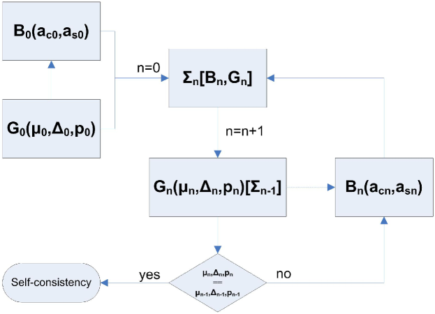
Figure 1: (Color online) Self-consistency scheme to compute the propagator $G$ in terms of the charge-charge and spin-spin propagator $B$ and the residual self-energy $\Sigma$.

II.6 Self-consistency

In this section, we will give a sketch of the procedure used to calculate the Green’s function $G(\mathbf{k},\omega)$. The starting point is equation (18), where the two matrices $I(\mathbf{k})$ and $\varepsilon(\mathbf{k})$ are computed by means of the expressions (22) and (23). The energy matrix $\varepsilon(\mathbf{k})$ depends on three parameters: $\mu$, $\Delta$, and $p$. To determine these parameters we use the following set of algebra constraints

$$\begin{array}[]{l}n=2(1-C_{11}-C_{22})\\ \Delta=C_{11}^{\alpha}-C_{22}^{\alpha}\\ C_{12}=\langle\xi(i)\eta^{\dagger}(i)\rangle=0\end{array}$$ (79)

where $C_{nm}$ and $C_{nm}^{\alpha}$ are the time-independent correlation functions $C_{nm}=\langle\psi_{n}(i)\psi_{m}^{\dagger}(i)\rangle$ and $C_{nm}^{\alpha}=\langle\psi_{n}^{\alpha}(i)\psi_{m}^{\dagger}(i)\rangle$. To calculate $\Sigma(\mathbf{k},\omega)$ we use the NCA; the results given in Sec. II.4 show that within this approximation $\Sigma(\mathbf{k},\omega)$ is expressed in terms of the fermionic $G_{cc}(\mathbf{k},\omega)$ [cfr. (39)] and of the bosonic $\chi_{\mu}(\mathbf{k},\omega)$ [cfr. (40)] propagators. The bosonic propagator is calculated within the two-pole approximation, using the expression (76). As shown in Sec. II.5, $\chi_{\mu}(\mathbf{k},\omega)$ depends on both electronic correlation functions [see (68)], which can be straightforwardly computed from $G(\mathbf{k},\omega)$, and bosonic correlation functions, one per each channel (charge and spin), $a_{0}$ and $a_{3}$. The latter are determined by means of the local algebra constraints (72), where $n$ is the filling and $D$ is the double occupancy, determined in terms of the electronic correlation function as $D=n/2-C_{22}$.

According to this, the electronic Green’s function $G(\mathbf{k},\omega)$ is computed through the self-consistency scheme depicted in Fig. 1: we first compute $G^{0}(\mathbf{k},\omega)$ and $\chi_{\mu}(\mathbf{k},\omega)$ in the two-pole approximation, then $\Sigma(\mathbf{k},\omega)$ and consequently $G(\mathbf{k},\omega)$. Finally, we check how much the fermionic parameters ($\mu$, $\Delta$, and $p$) changed and decide if to stop or to continue by computing new $\chi_{{}_{\mu}}(\mathbf{k},\omega)$ and $\Sigma(\mathbf{k},\omega)$ after $G(\mathbf{k},\omega)$. Usually, to get $6$ digits precision for fermionic parameters, we need $8$ full cycles to reach self-consistency on a 3D grid of $128\times 128$ points in momentum space and $4096$ Matsubara frequencies. Actually, many more cycles (almost twice) are needed at low doping and low temperatures.

Summarizing, within the NCA and the two-pole approximation for the computation of $\chi_{\mu}(\mathbf{k},\omega)$ we have constructed an analytical, completely self-consistent, scheme of calculation of the electronic propagator $G_{cc}(\mathbf{k},\omega)=\mathcal{F}\langle T[c(i)c^{\dagger}(j)]\rangle$, where dynamical contributions of the self-energy $\Sigma(\mathbf{k},\omega)$ are included. All the internal parameters are self-consistently calculated by means of algebra constraints [cfr. (72)-(73) and (79)]. No adjustable parameters or phenomenological expressions are introduced.

III Results

In the following, we analyze some electronic properties by computing the spectral function

$$A(\mathbf{k},\omega)=-\frac{1}{\pi}\Im[G_{cc}(\mathbf{k},\omega)]$$ (80)

the momentum distribution function per spin

$$n(\mathbf{k})=\int d\omega\,f_{\mathrm{F}}(\omega)A(\mathbf{k},\omega)$$ (81)

and the density of states per spin

$$N(\omega)=\frac{1}{(2\pi)^{2}}\int d^{2}kA(\mathbf{k},\omega)$$ (82)

where $G_{cc}(\mathbf{k},\omega)=G_{11}(\mathbf{k},\omega)+G_{12}(\mathbf{k},\omega)+G_{21}(\mathbf{k},\omega)+G_{22}(\mathbf{k},\omega)$ is the electronic propagator and $f_{\mathrm{F}}(\omega)$ is the Fermi function. We also study the electronic self-energy $\Sigma_{cc}(\mathbf{k},\omega)$, which is defined through the equation

$$G_{cc}(\mathbf{k},\omega)=\frac{1}{\omega-\epsilon_{0}(\mathbf{k})-\Sigma_{cc}(\mathbf{k},\omega)}$$ (83)

where $\epsilon_{0}(\mathbf{k})=-\mu-4t\alpha(\mathbf{k})$ is the non-interacting dispersion. Moreover, we define the quantity $r(\mathbf{k})=\epsilon_{0}(\mathbf{k})+\Sigma^{\prime}_{cc}(\mathbf{k},\omega=0)$ that determines the Fermi surface locus in momentum space, $r(\mathbf{k})=0$, in a Fermi liquid, i.e. when $\lim_{\omega\rightarrow 0}\Sigma"_{cc}(\mathbf{k},\omega,T=0)\propto\omega^{2}$ and $\lim_{T\rightarrow 0}\Sigma"_{cc}(\mathbf{k},\omega=0,T)\propto T^{2}$. The actual Fermi surface (or its relic in a non-Fermi-liquid) is given by the relative maxima of $A(\mathbf{k},\omega=0)$, which takes into account, at the same time and on equal footing, both the real and the imaginary parts of the self-energy and is directly related, within the sudden approximation and forgetting any selection rules, to what ARPES effectively measures.

Finally, the spin-spin correlation function $\left\langle n_{z}n_{z}^{\alpha}\right\rangle$, the pole $\omega^{(3)}(\mathbf{k}=\mathbf{Q}=(\pi,\pi))$ of the spin-spin propagator and the antiferromagnetic correlation length $\xi$. are discussed. Usually, the latter is defined by supposing the following asymptotic expression for the static susceptibility

$$\lim_{\mathbf{k}\to\mathbf{Q}}\chi^{(3)}\left(\mathbf{k},0\right)=\frac{\chi^{(3)}\left(\mathbf{Q},0\right)}{1+\xi^{2}\left|\mathbf{k-Q}\right|^{2}}$$ (84)

where $\chi^{(3)}\left(\mathbf{k},0\right)=-G^{(3)}\left(\mathbf{k},0\right)$. It is worth noting that in our case (84) is not assumed, but it exactly holds Avella and Mancini (2003).

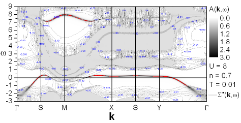
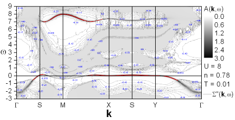
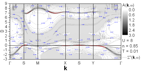
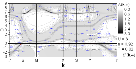
Figure 2: (Color online) Spectral function $A(\mathbf{k},\omega)$ along the principal directions ($\Gamma=(0,\,0)\to M=(\pi,\,\pi)$, $M\to X=(\pi,\,0)$, $X\to Y=(0,\,\pi)$ and $Y\to\Gamma$) for $U=8$, $T=0.01$ and (top) $n=0.70$, (middle top) $n=0.78$, (middle bottom) $n=0.85$ and (bottom) $n=0.92$ ($T=0.02$).

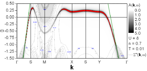
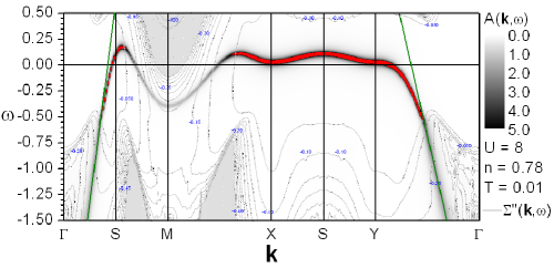
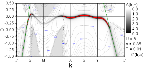
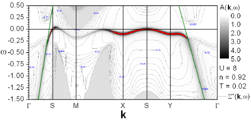
Figure 3: (Color online) Spectral function $A(\mathbf{k},\omega)$ close to the chemical potential ($\omega=0$) along the principal directions ($\Gamma=(0,\,0)\to M=(\pi,\,\pi)$, $M\to X=(\pi,\,0)$, $X\to Y=(0,\,\pi)$ and $Y\to\Gamma$) for $U=8$, $T=0.01$ and (top) $n=0.70$, (middle top) $n=0.78$, (middle bottom) $n=0.85$ and (bottom) $n=0.92$ ($T=0.02$).

III.1 Spectral Function and Dispersion

According to its overall relevance in the whole analysis performed hereinafter, we first discuss the electronic dispersion of the model under analysis or, better, its relic in a strongly correlated system. In general, the dispersion and its more or less anomalous features can be inferred by looking at the maxima of the spectral function $A(\mathbf{k},\omega)$. In Figs. 2 and 3, the spectral function is shown, in scale of grays (increasing from white to black; red is for above-scale values), along the principal directions ($\Gamma=(0,\,0)\to M=(\pi,\,\pi)$, $M\to X=(\pi,\,0)$, $X\to Y=(0,\,\pi)$ and $Y\to\Gamma$) for $U=8$, $T=0.01$ and (top) $n=0.70$, (middle top) $n=0.78$, (middle bottom) $n=0.85$ and (bottom) $n=0.92$ ($T=0.02$). In Fig. 2, the whole range of frequencies with finite values of $A(\mathbf{k},\omega)$ is reported, while in Fig. 3 a zoom in the proximity of the chemical potential is shown. The light gray lines and uniform areas are labeled with the values of the imaginary part of the self-energy $\Sigma^{\prime\prime}(\mathbf{k},\omega)$ and give one of the most relevant keys to interpret the characteristics of the dispersion. The dark green lines in Fig. 3 are just guides to the eye and indicate the direction of the dispersion just before the visible kink separating the black and the red areas of the dispersion.

The red areas, as they mark the relative maxima of $A(\mathbf{k},\omega)$, can be considered as the best possible estimates for the dispersion. In a non- (or weakly-) interacting system, the dispersion would be a single, continuos and (quite-)sharp line representing some function $\varepsilon\left(\mathbf{k}\right)$ being the simple pole of $G_{cc}(\mathbf{k},\omega)$. In this case (for a strongly correlated system), instead, we can clearly see that the dispersion is well-defined (red areas) only in some of the regions it crosses in the $(\mathbf{k},\omega)$ plane: the regions where $\Sigma^{\prime\prime}(\mathbf{k},\omega)$ is zero or almost negligible. In the crossed regions where $\Sigma^{\prime\prime}(\mathbf{k},\omega)$ is instead finite, $A(\mathbf{k},\omega)$ obviously assumes very low values, which would be extremely difficult (actually almost impossible) to detect by ARPES. Accordingly, ARPES would report only the red areas in the picture. This fact is fundamental to understand and describe the experimental findings regarding the Fermi surface in the underdoped regime, as they will discussed in the next section, and to reconcile ARPES findings with those of quantum oscillations measurements.

The two Hubbard sub-bands, separated by a gap of the order $U$ and with a reduced band-width of order $4t$, are clearly visible: the lower one (LHB) is partly occupied as it is crossed by the chemical potential, the upper one (UHB) is empty and very far from the chemical potential. The lower sub-band systematically (for each value of doping) loses significance close to $\Gamma$ and to $M$, although this effect is more and more pronounced on reducing doping. In both cases (close to $\Gamma$ and to $M$), $A(\mathbf{k},\omega)$ loses weight as $\Sigma^{\prime\prime}(\mathbf{k},\omega)$ increases its own: this can be easily understood if we recall that both $\chi_{0}\left(\mathbf{k},\omega\right)$ and $\chi_{3}\left(\mathbf{k},\omega\right)$ have a vanishing pole at $\Gamma$ (due to hydrodynamics) and that $\chi_{3}\left(\mathbf{k},\omega\right)$ is strongly peaked at $M$ due to the strong antiferromagnetic correlations present in the system (see Sec. III.6). The upper sub-band, according to the complementary effect induced by the evident shadow-bands appearance (signaled by the relative maxima of $\Sigma^{\prime\prime}(\mathbf{k},\omega)$ marked by $100$ and the dark gray area inside the gap) due again to the strong antiferromagnetic correlations present in the system, displays a well-defined dispersion at $M$, at least for high enough doping, and practically no dispersion at all close to $\Gamma$. For low doping, the great majority of the upper sub-band weight is simply transferred to the lower sub-band. The growth, on reducing doping, of the undefined-dispersion regions close to $\Gamma$ in the lower sub-band cuts down its already reduced bandwidth of order $4t$ to values of the order $J=\frac{4t^{2}}{U}=0.5t$, as one would expect for the dispersion of few holes in a strong antiferromagnetic background. The shape of the dispersion too is compatible with this scenario: the sequence of minima and maxima is compatible, actually driven, by the doubling of the Brillouin zone induced by the strong antiferromagnetic correlations, as well as the dynamical generation of a $t^{\prime}$ diagonal hopping (absent in the Hamiltonian currently under study) clearly signaled by the more and more, on reducing doping, pronounced warping of the dispersion along the $X\to Y$ direction (more evident in Fig. 3), which would be perfectly flat otherwise (for $t^{\prime}=0$).

Moving to the zooms (Fig. 3), they show much more clearly: the systematic reduction of the bandwidth on reducing doping, the doubling of the zone, the systematic increase of the warping along $X\to Y$ on reducing doping, the extreme flatness of the dispersion at $X$ coming from both $\Gamma$ and $M$. This latter feature is in very good agreement with quantum Monte Carlo calculations (see Bulut (2002) and references therein) as well as with ARPES experiments Yoshida et al. (2001), which report a similar behavior in the overdoped region. Moreover, they show that, in contrast with the scenario for a non- (or weakly-) interacting system, where the doubling of the zone happens with the $X\to Y$ direction as pivot, here the doubling is confined to the region close to $M$. The lower sub-band is completely filled at half-filling, while for an ordinary Slater antiferromagnet the gap opens at half-filling just on top of the van-Hove singularity along $X\to Y$. In addition, the effective, finite value of $t^{\prime}$ makes the dispersion maximum close to $S$ higher than the one present along the $M\to X$ direction, opening the possibility for the appearance of hole pockets close to $S$. Finally, it is now evident that the warping of the dispersion along $X\to Y$ will also induce the presence of two maxima in the density of states: one due to the van-Hove singularities at $X$ and $Y$ and one due to the maximum in the dispersion close to $S$. How deep is the dip between these two maxima just depends on the number of available well-defined (red) states in momentum present between these two values of frequency. This will determine the appearance of a more or less pronounced pseudogap in the density of states, but let us come back to this after having analyzed the region close to $M$.

As a matter of fact, it is just the absence of spectral weight in the region close to $M$ and, in particular and more surprisingly, at the chemical potential (i.e. on the Fermi surface, in contradiction with the Fermi-liquid picture), the main and more relevant result of this analysis: it will determine almost all interesting and anomalous/unconventional features of the single-particle properties of the model. The scenario emerging from this analysis can be relevant not only for the understanding of the physics of the Hubbard model and for the microscopical description of the cuprate high-$T_{c}$ superconductors, but also for the drafting of a general microscopic theory of strongly correlated systems. The strong antiferromagnetic correlations (through $\Sigma^{\prime\prime}(\mathbf{k},\omega)$, which mainly follows $\chi_{3}\left(\mathbf{k},\omega\right)$) cause a significative and anomalous/unconventional loss of spectral weight around $M$, which induces in turn: the deconstruction of the Fermi surface (Sec. III.2), the emergence of momentum selective non-Fermi liquid features (Secs. III.4 and III.5), and the opening of a well-developed (deep) pseudogap in the density of states (Sec. III.3).

Last, but not least, it is also remarkable the presence of kinks in the dispersion in both the nodal ($\Gamma\to M$) and the antinodal ($X\to\Gamma$) directions, as highlighted by the dark green guidelines, in qualitative agreement with some ARPES experiments Damascelli et al. (2003). Such a phenomenon clearly signals the coupling of the electrons to a bosonic mode. In this scenario, the mode is clearly magnetic in nature. The frequency of the kink, with respect to the chemical potential, reduces systematically and quite drastically on reducing doping, following the behavior of the pole of $\chi_{3}\left(\mathbf{k},\omega\right)$ (see Sec. III.6). Combining the presence of kinks and the strong reduction of spectral weight below them, we see the appearance of waterfalls, in particular along the antinodal ($X\to\Gamma$) direction, as found in some ARPES experiments Damascelli et al. (2003). Finally, the extension of the flat region in the dispersion around the antinodal points ($X$ and $Y$) , i.e. at the van-Hove points, increases systematically on decreasing doping. This clearly signals the transfer of spectral weight from the Fermi surface, which is depleted by the strong antiferromagnetic fluctuations, which are also responsible for the remarkable flatness of the band edge.

Before moving to the next section, it is worth noticing that similar results for the single-particle excitation spectrum (flat bands close to $X$, weight transfer from the LHB to the UHB at $M$, splitting of the band close to $X$, …) were obtained within the self-consistent projection operator method Kakehashi and Fulde (2004, 2005), the operator projection method Onoda and Imada (2001a, b, 2003) and within a Mori-like approach by Plakida and coworkers Plakida and Oudovenko (2007); Plakida (2010).

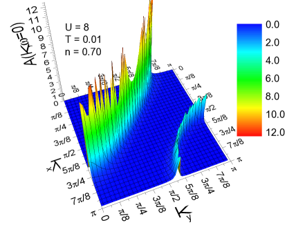
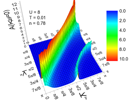
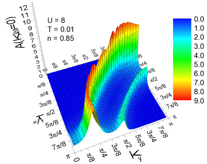
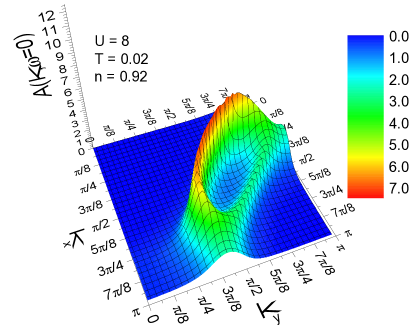
Figure 4: (Color online) Spectral function at the chemical potential $A(\mathbf{k},\omega=0)$ as a function of momentum $\mathbf{k}$ for $U=8$, $T=0.01$ and (top left) $n=0.70$, (top right) $n=0.78$, (bottom left) $n=0.85$ and (bottom right) $n=0.92$ ($T=0.02$).

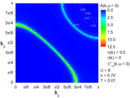
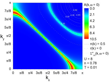
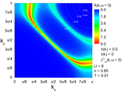
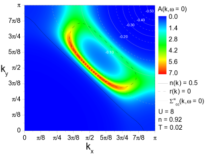
Figure 5: (Color online) Spectral function at the chemical potential $A(\mathbf{k},\omega=0)$ as a function of momentum $\mathbf{k}$ for $U=8$, $T=0.01$ and (top) $n=0.70$, (middle top) $n=0.78$, (middle bottom) $n=0.85$ and (bottom) $n=0.92$ ($T=0.02$). The solid line marks the locus $n(\mathbf{k})=0.5$, the dashed line marks the locus $r(\mathbf{k})=0$, the gray lines are labeled with the values of $\Sigma^{\prime\prime}_{cc}(\mathbf{k},\omega=0)$, and the dotted line is a guide to the eye and marks the reduced (antiferromagnetic) Brillouin zone.

III.2 Spectral Function and Fermi Surface

Focusing on the value of the spectral function at the chemical potential, $A(\mathbf{k},\omega=0)$, we can discuss the closest concept to Fermi surface available in a strongly correlated system. In Fig. 4, $A(\mathbf{k},\omega=0)$ is plotted as a function of the momentum $\mathbf{k}$ in a quarter of the Brillouin zone for $U=8$ and four different couples of values of temperature and filling: (top left) $n=0.7$ and $T=0.01$, (top right) $n=0.78$ and $T=0.01$ , (bottom left) $n=0.85$ and $T=0.01$ and (bottom right) $n=0.92$ and $T=0.02$. The Fermi surface, in agreement with the interpretation of the ARPES measurements within the sudden approximation, can be defined as the locus in momentum space of the relative maxima of $A(\mathbf{k},\omega=0)$. Such a definition opens up the possibility to explain ARPES measurements, but also to go beyond them and their finite instrumental resolution and sensitivity with the aim at filling the gap with other kind of measurements, in particular quantum oscillations ones, which seems to report results in disagreement, up to dichotomy in some cases, with the scenario depicted by ARPES.

For each value of the filling reported, we can easily distinguish two walls/arcs; for $n=0.92$, they somewhat join. First, let us focus on the arc with the larger (by far) intensities; given the current sensitivities, this is the only one, among the two, possibly visible to ARPES. At $n=0.7$ (see Fig. 4 (top left panel)), the 3D perspective allows to better appreciate the difference in the intensities of the relative maxima of $A(\mathbf{k},\omega=0)$ between the region close to the main diagonal ($M\to X$), where the signal is weaker, and the regions close to the main axes ($\Gamma\to X$ and $\Gamma\to Y$), where the signal is stronger; this behavior has been also reported by ARPES experiments Yoshida et al. (2001); Damascelli et al. (2003) as well as the electron-like nature of the Fermi surface Yoshida et al. (2001). On decreasing doping, this trend reverses, passing through $n=0.78$, where the intensities almost match, and up to $n=0.92$, where the region in proximity of $S$ is the only one with an appreciable signal. The less-intense (by far) arc, reported in Ref. Plakida and Oudovenko (2007) too, is the relic of a shadow band, as can be clearly seen in Fig. 3, and, consequently, never changes its curvature, in contrast to what happens to the other arc, which is subject to the crossing of the van Hove singularity ($n\cong 0.82$) instead. Although the ratio between the maximum values of the intensities at the two arcs never goes below two (see Fig 6 (right panel)), there is an evident decrease of the maximum value of the intensity at the larger-intensity arc on decreasing doping, which clearly signals an overall increase of the intensity and/or of the effectiveness (in terms of capability to affect the relevant quasi-particles, which are those at the Fermi surface) of the correlations.

Moving to a 2D perspective (see Fig. 5), we can add three ingredients to our discussion that can help us better understanding the evolution with doping of the Fermi surface: (i) the $n(\mathbf{k})=0.5$ locus (solid line), i.e. the Fermi surface if the system would be non-interacting; (ii) the $r(\mathbf{k})=0$ locus (dashed line), i.e. the Fermi surface if the system would be a Fermi liquid or somewhat close to it conceptually; (iii) the values (grey lines and labels) of the imaginary part of the self-energy at the chemical potential $\Sigma^{\prime\prime}_{cc}(\mathbf{k},\omega=0)$ (notice that $T\neq 0$). Combining these three ingredients with the positions and intensities of the the relative maxima of $A(\mathbf{k},\omega=0)$, we can try to better understand what these latter signify and to classify the behavior of the system on changing doping. At $n=0.7$ (see Fig. 5 (top left panel)), the positions of the two arcs are exactly matching $r(\mathbf{k})=0$ lines; this will stay valid at each value of the filling reported, with a fine, but very relevant, distinction at $n=0.92$. This occurrence makes our definition of Fermi surface robust, but also versatile as it permits to go beyond Fermi liquid picture without contradicting this latter. The almost perfect coincidence, for the higher value of doping reported, $n=0.7$, of the $n(\mathbf{k})=0.5$ line with the larger-intensity arc clearly asserts that we are dealing with a very-weakly-interacting Fermi metal. $\Sigma^{\prime\prime}_{cc}(\mathbf{k},\omega=0)$ is quite large close to $M$ (see Fig. 3 (top panel)) and eats up the weight of the second arc, which becomes a ghost band more than a shadow one. The antiferromagnetic correlations are definitely finite (see Sec. III.6) and, consequently, lead to the doubling of the zone, but not strong enough to affect the behavior of the ordinary quasi-particles safely living at the ordinary Fermi surface. Decreasing the doping, we can witness a first topological transition from a Fermi surface closed around $\Gamma$ (electron like - hole like in cuprates language) to a Fermi surface closed around $M$ (hole like - electron like in cuprates language) at $n\cong 0.82$, where the chemical potential crosses the van Hove singularity (see Fig. 3). The chemical potential presents an inflection point at this doping (not shown), which allowed us to determine its value with great accuracy. In proximity of the antinodal points ($X$ and $Y$), a net discrepancy between the position of the relative maxima of $A(\mathbf{k},\omega=0)$ and the locus $n(\mathbf{k})=0.5$ becomes more and more evident on decreasing doping (see Fig. 5 (top right and bottom left panels)). This occurrence does not only allows the topological transition, which is absent for the $n(\mathbf{k})=0.5$ locus that reaches the anti-diagonal ($X\to Y$) at half-filling in agreement with the Luttinger theorem, but it also accounts for the apparent broadening of the relative maxima of $A(\mathbf{k},\omega=0)$ close to the anti-nodal points ($X$ and $Y$). The broadening is due to the small, but finite, value of $\Sigma^{\prime\prime}_{cc}(\mathbf{k},\omega=0)$ in those momentum regions (see Fig. 3 (middle panels)), signaling the net increase of the correlation strength and, accordingly, the impossibility to describe the system in this regime as a conventional non- (or weakly-) interacting system within a Fermi-liquid scenario or its ordinary extensions for ordered phases. What is really interesting and goes beyond the actual problem under analysis (cuprates - 2D Hubbard model), is the emergence of such features only in well defined regions in momentum space. This selectiveness in momentum is quite a new feature in condensed matter physics and its understanding and description require quite new theoretical approaches. In this system, almost independently from their effective strength, the correlations play a so fundamental role to come to shape and determine qualitatively the response of the system. Accordingly, any attempt to treat correlations without taking into account the level of entanglement between all degrees of freedom present in the system is bound to fail or at least to miss the most relevant features.

Let us come to the most interesting result. At $n=0.92$, the relative maxima of $A(\mathbf{k},\omega=0)$ detach also from the $r(\mathbf{k})=0$ locus, at least partially, opening a completely new scenario. $r(\mathbf{k})=0$ defines a pocket (close, but absolutely not identical - read below, to that of an antiferromagnet), while the relative maxima of $A(\mathbf{k},\omega=0)$ feature the very same pocket together with quite broad, but still well-defined, wings closing with one half of the pocket (the most intense one) what can be safely considered the relic of a large Fermi surface. This is the second and most surprising topological transition occurring to the actual Fermi surface: the two arcs, clearly visible for all other values of the filling, join and instead of closing just a pocket, as one would expect on the basis of the conventional theory for an antiferromagnet - here mimed by $r(\mathbf{k})=0$ locus, develop (or keep) a completely independent branch. The actual Fermi surface is neither a pocket nor a large Fermi surface; for a more expressive representation see Fig. 4 (bottom right panel). This very unexpected result can be connected to the dichotomy between those experiments (e.g. ARPES) pointing to a small and those ones (e.g. quantum oscillations) pointing to a large Fermi surface. This result can be understood by looking once more at the dispersion for this value of the filling (see Fig. 3 (bottom panel)): the difference in height, induced by the effective finite value of $t^{\prime}$, which increases with decreasing doping, between the two highest maxima in the dispersion - one close to $S$ and the other along the $M\to X$ direction - makes the latter to cross the chemical potential for larger values of the doping than the first, but given the significative broadening of the dispersion, even when the center mass of the second leaves the Fermi surface (disappearing from $r(\mathbf{k})=0$ locus), its shoulders are still active and well-identifiable at the chemical potential - that is on the actual Fermi surface.

The pocket too is far from being conventional. It is clearly evident in Fig. 5 (bottom right panel) that there are two distinct halves of the pocket: one with very high intensity pinned at $S$ (again the only possibly visible to ARPES) and another with very low intensity (visible only to theoreticians and some quantum oscillations experiments). This is our interpretation for the Fermi arcs reported by many ARPES experimentsDamascelli et al. (2003); Shen et al. (2005) and unaccountable for any ordinary theory relaying on the Fermi liquid picture, although modified by the presence of an incipient spin or charge ordering. Obviously, looking only at the Fermi arc (as ARPES is forced to do), the Fermi surface looks ill defined as it does not enclose a definite region of momentum space, but having access also to the other half of the pocket, such problem is greatly alleviated. The point is that the antiferromagnetic fluctuations are so strong to destroy the coherence of the quasi-particles in that region of momentum space as similarly reported within the DMFT$+\Sigma$ approach Sadovskii (2001); Sadovskii et al. (2005); Kuchinskii et al. (2005, 2006, 2007) and a Mori-like approach by Plakida and coworkers Plakida and Oudovenko (2007); Plakida (2010). Moreover, we will see that (see Sec. III.5), the phantom half is not simply lower in intensity because it belongs to a shadow band depleted by a finite imaginary part of the self-energy (see Fig. 5 (bottom right panel)), but that it lives in a region of momentum where the imaginary part of the self-energy shows clear signs of non-Fermi liquid behavior. The lack of next-nearest hopping terms (i.e., $t^{\prime}$ and $t^{\prime\prime}$) in the chosen Hamiltonian (1), although they are evidently generated dynamically, does not allow us to perform a quantitative comparison between our results and the experimental ones, which refers to a specific material characterized by a specific set of hoppings. This also explains why our Fermi arc is pinned at $S$ and occupies the outer reduced Brillouin zone, while many experimental results report a Fermi arc occupying the inner reduced Brillouin zone. Actually, the pinning (with respect to doping within the underdoped region) of the center of mass of the ARPES-visible Fermi arc has been reported also from ARPES experimentsKoitzsch et al. (2004).

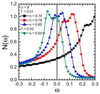
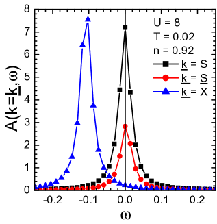
Figure 6: (Color online) (left) Density of states $N(\omega)$ as a function of frequency $\omega$ for $U=8$, (black squares) $n=0.7$ and $T=0.01$, (red circles) $n=0.78$ and $T=0.01$, (blue up triangles) $n=0.85$ and $T=0.01$, and (green down triangles) $n=0.92$ and $T=0.02$. (right) Spectral function in proximity of the chemical potential $A(\mathbf{\underline{k}},\omega\sim 0)$ at (black squares) $\mathbf{\underline{k}}=S=(\pi/2,\pi/2)$, (red circles) $\underline{S}$ (in the text), and (blue triangles) $X=(\pi,\,0)$ for $U=8$, $n=0.92$ and $T=0.02$.

III.3 Density of States and Pseudogap

The other main issue in the underdoped regime of cuprates superconductors is the presence of a quite strong depletion in the electronic density of states, known as pseudogap. In Fig. 6 (left panel), we report the density of states $N(\omega)$ for $U=8$ and four couples of values of filling and temperature: $n=0.7$ and $T=0.01$, $n=0.78$ and $T=0.01$, $n=0.85$ and $T=0.01$, and $n=0.92$ and $T=0.02$, in the frequency region in proximity of the chemical potential. As a reference, we also report, in Fig. 6 (right panel), the spectral function in proximity of the chemical potential $A(\mathbf{\underline{k}},\omega\sim 0)$ at $\mathbf{\underline{k}}=S=(\pi/2,\pi/2)$, $\mathbf{\underline{k}}=\underline{S}$ which lies where the phantom half of the pocket touches the main diagonal $\Gamma\to M$ (i.e. where the dispersion cuts the main diagonal $\Gamma\to M$ closer to $M$), and $\mathbf{\underline{k}}=X=(\pi,\,0)$ for $U=8$, $n=0.92$ and $T=0.02$. As it can be clearly seen in Fig. 6 (left panel), the density of states present two maxima separated by a dip, which plays the role of pseudogap in this scenario. Its presence is due to the warping in the dispersion along the $X\to Y$ direction (see Fig. 3), which induces the presence of the two maxima (one due to the van-Hove singularity at $X$ and one due to the maximum in the dispersion close to $S$ - see Fig. 6 (right panel)), and to the loss of states, within this window in frequency, in the region in momentum close to $M$, as discussed in detail in the previous sections. As a measure of how much weight is lost because of the finite value of the imaginary part of the self-energy in the region in momentum close to $M$, one can look at the striking difference between the value of $A(\underline{S},\omega=0)$ in comparison to that of $A(S,\omega=0)$, see Fig. 6 (right panel). On reducing the doping, there is an evident transfer of spectral weight between the two maxima; in particular, the weight is transferred from the top of the dispersion close to $S$ to the antinodal point $X$, where the van Hove singularity resides. At the lowest doping ($n=0.92$), a well developed pseudogap is visible below the chemical potential and will clearly affect all measurable properties of the system. For this doping, we do not observe any divergence of $\Sigma^{\prime}_{cc}(\mathbf{k},\omega=0)$ in contrast to what reported in Ref. Stanescu and Kotliar (2006) where this feature is presented as the ultimate reason for the opening of the pseudogap. In our scenario, the pseudogap is just the result of the transfer of weight from the single-particle density of states to the two-particle one related to the (antiferro)magnetic excitations developing in the system on decreasing doping at low temperatures (see Sec. III.6).

It is worth mentioning that an analogous doping behavior of the pseudogap has been found by the DMFT$+\Sigma$ approach Sadovskii (2001); Sadovskii et al. (2005); Kuchinskii et al. (2005, 2006, 2007), a Mori-like approach by Plakida and coworkers Plakida and Oudovenko (2007); Plakida (2010) and the cluster perturbation theory Sénéchal et al. (2000); Sénéchal and Tremblay (2004); Tremblay et al. (2006).

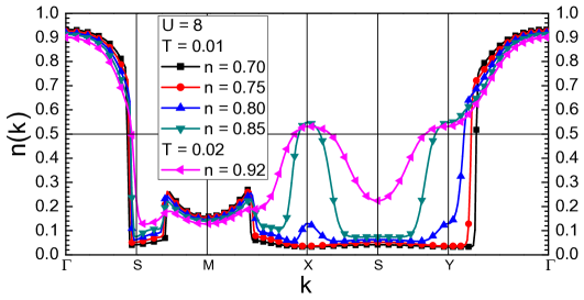
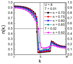
Figure 7: (Color online) Momentum distribution function $n(\mathbf{k})$ for $U=8$ and $n=0.7$, $0.75$, $0.8$, $n=0.85$ ($T=0.01$), and $n=0.92$ ($T=0.02$): (left) along the principal directions ($\Gamma=(0,\,0)\to M=(\pi,\,\pi)$, $M\to X=(\pi,\,0)$, $X\to Y=(0,\,\pi)$ and $Y\to\Gamma$); (right) along the principal diagonal ($\Gamma\to M$).

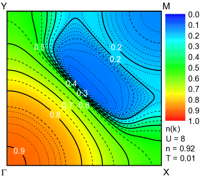
Figure 8: (Color online) The momentum distribution function $n(\mathbf{k})$ for $n=0.92$, $T=0.01$ and $U=8$.

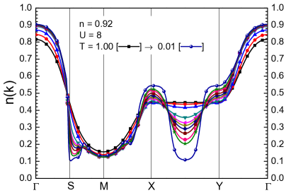
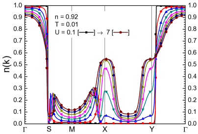
Figure 9: (Color online) The momentum distribution function $n(\mathbf{k})$ along the main directions ($\Gamma=(0,0)$ $\to$ $M=(\pi,\pi)$ $\to$ $X=(\pi,0)$ $\to$ $Y=(0,\pi)$ $\to$ $\Gamma=(0,0)$) for different values of temperature $T$ (left) and on-site Coulomb repulsion $U$ (right) at $n=0.92$.

III.4 Momentum Distribution Function

To analyze a possible crossover from a Fermi liquid to a non-Fermi liquid behavior in certain regions of momentum space, at small dopings and low temperatures, and to better characterize the pocket forming on the Fermi surface at the lowest reported doping, we study the electronic momentum distribution function $n(\mathbf{k})$ per spin along the principal directions ($\Gamma\to M$, $M\to X$, $X\to Y$ and $Y\to\Gamma$) and report it in Fig. 7, for $U=8$ and $n=0.7$, $0.75$, $0.8$, and $0.85$ ($T=0.01$), and for $n=0.92$ ($T=0.02$). The right panel in the figure reports a zoom along the main diagonal ($\Gamma\to M$). At the highest studied doping ($n=0.7$), $n(\mathbf{k})$ shows the usual features of a quasi non-interacting system, except for one single, but very important feature: the dip along the main diagonal ($\Gamma\to M$) signaling the presence of a shadow band due to the weak, but anyway finite, antiferromagnetic correlations (see Sec. III.6), as already discussed many times hereinbefore. The quite small height of the secondary jumps along $S\to M$ and $M\to X$ directions (with respect to the height of the main jumps along $\Gamma\to S$ and $Y\to\Gamma$ directions) gives a measure of the relevance of this feature in the overall picture: not really much relevant, except at $n=0.92$ where it changes qualitatively. On increasing filling (reducing doping), the features related to the shadow band do not change much their positions and intensity, while the features related to the ordinary band change their positions as expected in order to accommodate (i.e. to activate states in momentum for) the increasing number of particles. Finally, at $n=0.92$, the two sets of features close a pocket. At this final stage, what is very relevant, as it is very unconventional, is the evident and remarkable difference in behavior between the main jump along the $\Gamma\to S$ direction and the secondary jump along the $S\to M$ direction (see Fig. 7 (right panel)): the former stays quite sharp (just a bit skewed by the slightly higher temperature) as the Fermi liquid theory requires, the latter instead loses completely its sharpness, much more than what would be reasonable because of the finite value of the temperature as it can be deduced by the comparison with the behavior of the main jump. Such a strong qualitative modification is the evidence of a non-Fermi-liquid-like kind of behavior, but only combining this occurrence with a detailed study of the frequency and temperature dependence of the imaginary part of the self-energy in the very same region of momentum space (see Sec. III.5), we will be able to make a definitive statement about this.

In Fig. 8, we try to summarize the scenario in the extreme case ($n=0.92$, $T=0.01$ and $U=8$), where all the anomalous features are present and well formed, by reporting the full 2D scan of the momentum distribution function $n(\mathbf{k})$ in a quarter of the Brillouin zone. We can clearly see now the pocket with its center along the main diagonal and the lower border touching the border of the magnetic zone at exactly $S=(\pi/2,\pi/2)$. Actually, the 2D prospective makes more evident that there is a second underlying Fermi surface that corresponds to the ordinary paramagnetic one for this filling $n=0.92$ (large and hole-like) and touching the border of the zone between $M=(\pi,\pi)$ and $X=(\pi,0)$ ($Y=(0,\pi)$). This corresponds to the very small jump in Fig. 9 (left panel) along the same direction. It is worth mentioning that a similar behavior of the momentum distribution function has been found by means of a Mori-like approach by Plakida and coworkers Plakida and Oudovenko (2007); Plakida (2010).

In Fig. 9, we study the dependence of the momentum distribution function $n(\mathbf{k})$ on the temperature $T$ (left panel) and the on-site Coulomb repulsion $U$ (right panel) by keeping the filling $n$ fixed at the most interesting value: $0.92$. At high temperatures (in particular, down to $T=0.4$), the behavior of $n(\mathbf{k})$ is that of a weakly correlated paramagnet (no pocket along the $S\to M$ direction, no warping along the $X\to Y$ direction). For lower temperatures, the pocket develops along the $S\to M$ direction and the signal along the $X\to Y$ direction is no more constant, signaling the dynamical generation of a diagonal hopping term $t^{\prime}$, connecting same-spin sites in a newly developed antiferromagnetic background unwilling to be disturbed. In fact, such a behavior is what one expects when quite strong magnetic fluctuations develop in the system and corresponds to a well defined tendency towards an antiferromagnetic phase (see Sec. III.6). The $M$ point becomes another minimum in the dispersion in competition with $\Gamma$ and the dispersion should feature a maximum between them in correspondence to the center of the pocket. The whole bending of the dispersion confines the van Hove singularity below the Fermi surface in a open pocket (it closes out of the actually chosen Brillouin zone) visible in the momentum distribution as a new quite broad maximum at $X$ and $Y$. The dependence on $U$ shows that for $n=0.92$ and $T=0.01$, our solution presents quite strong antiferromagnetic fluctuations for every finite value of the Coulomb repulsion, although the two kind of pockets discussed just above are not well formed for values of $U$ less than $U=3\div 4$.

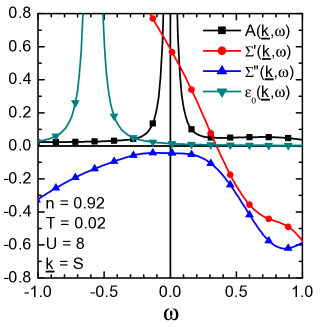
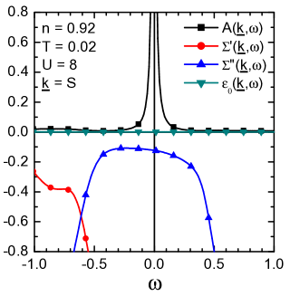
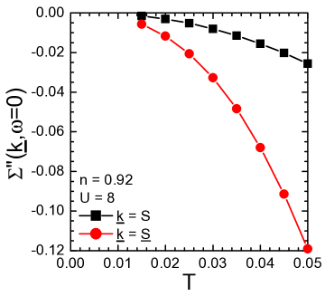
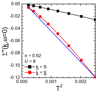
Figure 10: (Color online) Spectral density function $A\left(\underline{\mathbf{k}},\omega\right)$, real (^′) and imaginary (^′′) part of the self-energy $\Sigma\left(\underline{\mathbf{k}},\omega\right)$, non-interacting dispersion $\varepsilon_{0}\left(\underline{\mathbf{k}},\omega\right)$ as functions of frequency at (top left) $\underline{\mathbf{k}}=S$ and (top right) $\underline{\mathbf{k}}=\underline{S}$ for $n=0.92$, $T=0.02$ and $U=8$. (bottom) Imaginary part of the self-energy $\Sigma^{\prime\prime}\left(\underline{\mathbf{k}},\omega=0\right)$ as function of temperature at (squares) $\mathbf{k}=S$ and (circles) $\mathbf{k}=\underline{S}$ for $n=0.92$ and $U=8$. The blue line is just a guide to the eye.

III.5 Self-energy

To obtain clear-cut pieces of information about the lifetime of the quasi-particles generated by the very strong interactions within this scenario, but even more to understand if it is still reasonable or not to discuss in terms of quasi-particles at all (i.e. if this Fermi-liquid-like concept still holds for each region of the momentum and frequency space), we analyze the imaginary part of the self-energy $\Sigma^{\prime\prime}\left(\mathbf{k},\omega\right)$ as a function of both frequency and temperature. In the top panels of Fig. 10, we plot the imaginary part of the self-energy $\Sigma^{\prime\prime}\left(\underline{\mathbf{k}},\omega\right)$, together with its real part $\Sigma^{\prime}\left(\underline{\mathbf{k}},\omega\right)$, the spectral function $A(\underline{\mathbf{k}},\omega)$ and the non-interacting dispersion $\varepsilon_{0}\left(\underline{\mathbf{k}},\omega\right)$ as functions of the frequency at the nodal point $\underline{\mathbf{k}}=S$ (left panel) and at its companion position on the phantom half of the pocket $\underline{\mathbf{k}}=\underline{S}$ (right panel) along the main diagonal $\Gamma\to M$. In both cases, although for $\underline{\mathbf{k}}=\underline{S}$ is not visible in the picture, but is very clear for $\underline{\mathbf{k}}=S$, the position of the relative/local maximum of $A(\underline{\mathbf{k}},\omega)$ coincides with the chemical potential (i.e. where are on the Fermi surface) and it is determined by the sum of $\varepsilon_{0}\left(\underline{\mathbf{k}},\omega=0\right)$ and $\Sigma^{\prime}\left(\underline{\mathbf{k}},\omega=0\right)$ as expected (i.e. both points belong to the $r(\mathbf{k})=0$ locus). What is very interesting and somewhat unexpected and peculiar, is that at the nodal point a parabolic-like (i.e. a Fermi-liquid-like) behavior of $\Sigma^{\prime\prime}\left(\underline{\mathbf{k}},\omega\right)$ is clearly apparent, whereas at $\underline{\mathbf{k}}=\underline{S}$, the dependence of $\Sigma^{\prime\prime}\left(\underline{\mathbf{k}},\omega\right)$ on frequency shows a predominance of a linear term giving a definite proof that this region in momentum space is interested to a kind of physics very different from what can be considered even by far Fermi-liquid like.

In order to remove any possible doubt regarding the non-Fermi-liquid-like nature of the physics going on at the phantom half of the pocket, in the bottom panels of Fig. 10, the imaginary part of the self-energy at the Fermi surface $\Sigma^{\prime\prime}\left(\underline{\mathbf{k}},\omega=0\right)$ is reported as a function of the temperature at the nodal point $\underline{\mathbf{k}}=S$ and at its companion $\underline{\mathbf{k}}=\underline{S}$. The blue straight line in the right panel is just a guide to the eye. We clearly see that in this case too, although it requires to move from a $T$ to a $T^{2}$ representation (from left to right panel), the behavior of $\Sigma^{\prime\prime}\left(\underline{\mathbf{k}},\omega=0\right)$ shows rather different behaviors at the selected points. In particular, the temperature dependence of $\Sigma^{\prime\prime}\left(\underline{\mathbf{k}},\omega=0\right)$ is exactly parabolic (i.e., exactly Fermi-liquid) at the nodal point, while it exhibits a predominance of linear and logarithmic contributions at $\underline{S}$. This is one of the most relevant results of this analysis and characterize this scenario with respect to the others present in the literature.

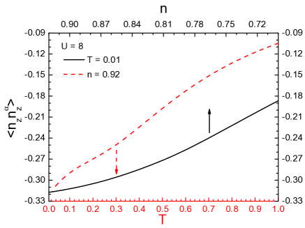
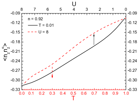
Figure 11: (Color online) The spin-spin correlation function $\left\langle n_{z}n_{z}^{\alpha}\right\rangle$ as a function of filling $n$, temperature $T$ and on-site Coulomb repulsion $U$ in the ranges $0.7<n<0.92$, $0.01<T<1$ and $0.1<U<8$.

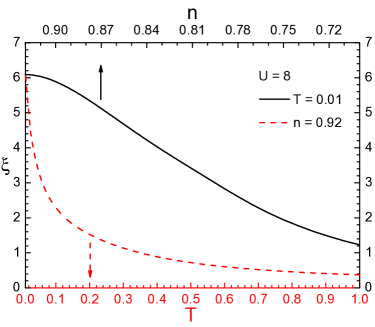
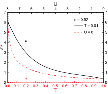
Figure 12: (Color online) The antiferromagnetic correlation length $\xi$ as a function of filling $n$, temperature $T$ and on-site Coulomb repulsion $U$ in the ranges $0.7<n<0.92$, $0.01<T<1$ and $0.1<U<8$.

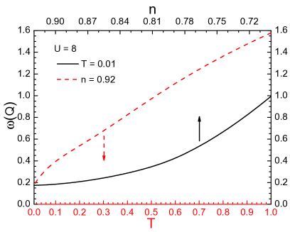
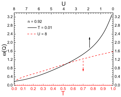
Figure 13: (Color online) The pole $\omega^{(3)}(\mathbf{Q})$ of the spin-spin propagator as a function of filling $n$, temperature $T$ and on-site Coulomb repulsion $U$ in the ranges $0.7<n<0.92$, $0.01<T<1$ and $0.1<U<8$.

III.6 Spin dynamics

Finally, to analyze the way the system approaches the antiferromagnetic phase on decreasing doping and temperature and increasing correlation strength, we report the behavior of the nearest neighbor spin-spin correlation function $\left\langle n_{z}n_{z}^{\alpha}\right\rangle$, of the antiferromagnetic correlation length $\xi$ and of the pole $\omega^{(3)}(\mathbf{Q})$ (as defined in Sec. III) as functions of filling $n$, temperature $T$ and on-site Coulomb repulsion $U$. In Figg. 11, 12 and 13, respectively, such quantities are presented for values in the ranges $0.7<n<0.92$, $0.01<T<1$ and $0.1<U<8$. The choice for the extremal values of low doping $n=0.92$, low temperature $T=0.01$ and strong on-site Coulomb repulsion $U=8$ has been made as for these values we find that all investigated single-particle properties (spectral density function, Fermi surface, dispersion relation, density of states, momentum distribution function, self-energy, …) present anomalous behaviors. The nearest-neighbor spin-spin correlation function $\left\langle n_{z}n_{z}^{\alpha}\right\rangle$ is always antiferromagnetic in character (i.e. negative) and increases its absolute value on decreasing doping and temperature $T$ and on increasing $U$ as expected. It is rather evident the signature of the exchange scale of energy $J\approx\frac{4t^{2}}{U}\approx 0.5$ in the temperature dependence as a significative enhancement in the slope. The analysis of the filling dependence unveils quite strong correlations at the higher value of doping too: $\xi$ is always larger than one for all values of fillings showing that, at $T=0.01$ and $U=8$, we should expect antiferromagnetic fluctuations in the overdoped regime too as also claimed by recent experiments Le Tacon et al. (2013); Dean et al. (2013); Jia et al. (2014). In the overdoped region, the antiferromagnetic fluctuations are quite less well defined, in terms of magnon/paramagnon width, than in the underdoped region Jaklič and Prelovšek (1995a, b); Vladimirov et al. (2009) and than what found in the current two-pole approximation. In fact, a proper description of the paramagnons dynamics would definitely require the inclusion of a proper self-energy term in the charge and spin propagators too (in preparation). Coming back to results (Fig. 12), $\xi$ overcomes one lattice constant at temperatures below $J$ and tends to diverge for low enough temperatures. On the other hand, $\xi$ seems to saturate for low enough values of doping. $\xi$ equals one between $U=3$ and $U=4$ and again rapidly increases for large enough values of $U$. The pole $\omega^{(3)}(\mathbf{Q})$ decreases on decreasing doping $n$ and temperature $T$ and on increasing $U$. In particular, it is very sensitive to the variations in temperature $T$ and in on-site Coulomb repulsion $U$, which make the mode softer and softer clearly showing the definite tendency towards an antiferromagnetic instability.

IV Conclusions and Perspectives

We have reviewed and systematized the theory and the results for the single-particle and the magnetic-response properties microscopically derived for the 2D Hubbard model, as minimal model for high-$T_{c}$ cuprate superconductors, within the Composite Operator Method with the residual self-energy computed in the Non-Crossing Approximation (NCA).

Among the several scenarios proposed for the pseudogap origin Norman et al. (2005), COM definitely falls into the AF scenario (the pseudogap is a precursor of the AF long-range order) Kampf and Schrieffer (1990); Schmalian et al. (1999); Abanov et al. (2003) as well as the two-particle self-consistent approach (TPSC) Vilk and Tremblay (1995); Tremblay et al. (2006), the DMFT$+\Sigma$ approach Sadovskii (2001); Sadovskii et al. (2005); Kuchinskii et al. (2005, 2006, 2007) and a Mori-like approach by Plakida and coworkers Plakida et al. (2003); Plakida and Oudovenko (2007); Plakida (2010).

In the limit of strong on-site Coulomb repulsion and low doping, such results show the emergence of a pseudogap scenario, the deconstruction of the Fermi surface in ill-defined open arcs and the clear signatures of non-Fermi-liquid features similarly to what has been found by ARPES experiments Damascelli et al. (2003) and not only Sebastian et al. (2012a). In particular, we have shown that a very low-intensity signal develops around $M$ point and moves towards $S$ nodal point on decreasing doping up to close, together with the ordinary Fermi surface boundary, a pocket in the underdoped region. Whenever the pocket develops, it is just the remarkable difference in the intensity of the signal between the two halves of the pocket to make a Fermi arc apparent. As the doping decreases further, the arc shrinks into a point at $S$ exactly at half filling making possible to reconcile the large-small Fermi surface dichotomy once the Fermi surface is defined as the relative maxima of the spectral function and the relic of the ordinary paramagnetic Fermi surface is also taken into account. The pseudogap develops since a region in momentum (and frequency) with a very low-intensity signal (it corresponds to the phantom half of the pocket at the chemical potential and to the shadow band out of it) is present between the van Hove singularity and the quite flat band edge (quite flat after the doubling of the Brillouin zone due to the very strong antiferromagnetic fluctuations). On changing doping, a spectral weight transfer takes place in the density of states between the two maxima corresponding to the van Hove singularity and the band edge, respectively. A crossover between a Fermi liquid and a non-Fermi liquid can be clearly observed in the momentum distribution function (definitely not featuring a sharp jump on the phantom half of the pocket) and in the imaginary part of the self-energy (featuring linear and logarithmic terms in the frequency and temperature dependence instead of the ordinary parabolic term) on decreasing doping at low temperatures and large interaction strength. This crossover exactly corresponds to the process of deconstruction of the Fermi surface. We also report kinks in the dispersion along nodal and anti-nodal directions. In order to properly interpret the behavior of the spectral density function and of the momentum distribution function, we have also analyzed the characteristic features in the spin-spin correlation function, the antiferromagnetic correlation length and the pole of the spin-spin propagator. As expected, on reducing doping or temperature and on increasing $U$, the correlations become stronger and stronger. The exchange scale of energy $J$ is clearly visible in the temperature dependence of the spin-spin correlation function and drives the overall behavior of the magnetic response. These results also demonstrate that a properly microscopically derived susceptibility can give results practically identical or, at least, very similar to those attainable by means of phenomenological susceptibilities specially tailored to describe experiments. This is even more remarkable since COM brings the benefice of a microscopical determination of the temperature and filling dependencies of the correlation length.

Many other issues should be addressed in the next future: to improve the Hamiltonian description by adding and fine tuning longer-range hopping terms in order to quantitatively and not only qualitatively describe specific materials, to verify the stability and the modifications of this scenario with respect to the inclusion of a residual self-energy in the calculation of the charge and spin propagators closing a fully self-consistent cycle, to investigate the charge and spin responses in the full range of momentum and frequency relevant for these systems searching for hourglasses, thresholds and all other peculiar features experimentally observed, to investigate the superconducting phase and establish it is nature and relationship with the anomalous features of the normal phases, to analyze in detail the transition/crossover between the quasi-ordinary antiferromagnetic phase at half-filling and the underdoped regime.