Explicit generation of the branching tree of states in spin glasses

Abstract

We present a numerical method to generate explicit realizations of the tree of states in mean-field spin glasses. The resulting study illuminates the physical meaning of the full replica symmetry breaking solution and provides detailed information on the structure of the spin-glass phase. A cavity approach ensures that the method is self-consistent and permits the evaluation of sophisticated observables, such as correlation functions. We include an example application to the study of finite-size effects in single-sample overlap probability distributions, a topic that has attracted considerable interest recently.

1 Introduction

Mean-field models in statistical mechanics usually have very compact solutions, which can be fully worked out in an analytical form, as a function of order parameters that solve simple self-consistency equations. In particular, the clustering property implies that connected correlations are weak enough within a pure state to allow for the computation of any correlation in terms of local fields, i.e., magnetizations and pairwise correlations (for models with 2-body interactions at most).

In spin-glass models the situation becomes definitely more complicated by the presence of a number of coexisting states, which is divergent in the thermodynamical limit for any temperature below the critical one, $T_{\mathrm{c}}$. Although correlations are still relatively simple within a state, the hierarchical structure of these states generates highly non-trivial correlations among local fields.

The order parameter in spin-glass models is the probability distribution $p_{J}(q)$ of the overlap $q$ between two copies of the system (to be better defined in the following), where the subindex $J$ denotes a particular realization of the disorer (a sample). The so-called Replica Symmetry Breaking (RSB) solution to mean-field spin-glass models [1, 2, 3] provides a self-consistency equation for the disorder-averaged $p(q)$. Although this is a partial differential equation, i.e., much more complicated than usual mean-field self-consistency equations, it can be solved with high accuracy [4]. In this way one can obtain precise results for many observables, such as the average free-energy, depending only on the average overlap distribution $p(q)$,

However, even though $p(q)$ encodes a lot of information about the system, translating a thorough knowledge of this function into physical results may be a non-trivial task. Let us consider a concrete example: suppose we want to understand whether a given model is well described within a given mean-field approximation. We can run Monte Carlo simulations for this model, take measurements of physical observables and compare them with the mean-field predictions. For example, one may be interested in studying local magnetizations, but this requires computing local fields that have non-trivial correlations in the RSB solution. How to compute them efficiently is one the aims of the present paper.

A second, and more relevant, example consists in the study of sample-to-sample fluctuations and finite-size effects. The main aim of this paper is showing how one can use a full knowledge of the $p(q)$ in order to generate explicitly different disorder realizations $p_{J}(q)$ in the thermodynamical limit and, then, how to introduce finite-size corrections so the analytical results can be directly compared to Monte Carlo simulations.

This is of great practical importance since the RSB solution can only be proven to hold for large spatial dimension ($D>6$). In the experimentally relevant $D=3$ system analytical methods are of only limited usefulness and Monte Carlo simulation emerges as a fundamental tool. Of course, the (necessarily) finite-size and finite-statistics results from a simulation will, at a glance, look very different from the analytical thermodynamical limit prediction, whether the system obeys RSB theory or not. In this situation, being able to extend the RSB prediction to finite sizes in a quantitative way is a major help.

The paper is organized as follows. In Section 2 we provide an extended introduction, summarizing what is known about the branching tree of states in mean-field spin glasses. In Section 3 we show how to generate one of these trees, while in Section 4 we explain how the cavity method can be exploited to reweight the trees and compute the, eventually unknown, correct branching factors. Finally in Section 5 we perform some tests to check our numerical implementation and in Section 6 we provide a practical application of the whole procedure to the problem of counting peaks in single-sample $p_{J}(q)$. The appendix discusses several technical improvements to the basic algorithm described in the text.

2 The branching structure of the tree of states

In this section we summarize the main results about the branching tree of states in mean-field spin glasses, in order to provide a self-contained introduction and to fix our notation. Most of the material in this section is well known in the literature, but not always accessible in a concise way, so we think it may be of use to a general reader that is not very familiar with the intricacies of the RSB theory. For a more detailed account and derivations, we refer the reader to Refs. [5, 6].

We start by considering the Sherrington-Kirkpatrick (SK) model [7]

$$\mathcal{H} = -\sum_{i,j}\sigma_{i}J_{ij}\sigma_{j},\quad\sigma_{i}=\pm 1,\quad i=1,\ldots,N,$$ (1)

where the quenched couplings $J_{ij}$ are independent, identically distributed (i.i.d.) random variables taken from a symmetric distribution with variance $1/N$. Since this system has a quenched disorder, we have to consider first the thermal average $\langle\cdots\rangle$ for a fixed choice of the $\{J_{ij}\}$ and then the average over all the possible disorder realizations, denoted with an overline, $\overline{(\cdots)}$.

Even though this is a mean-field model (its finite-dimensional counterpart, the Edwards-Anderson model [8], considers only short-range interactions), it has proven to be very complex. Indeed, even though the model was solved by Parisi in the early 1980s [1, 2, 3] using the replica symmetry breaking (RSB) method, a rigorous proof has been obtained only recently by Talagrand [9].

The RSB picture for the SK spin glass describes a system that experiences a second-order spin-glass transition at a temperature $T_{\mathrm{c}}=1$. Below $T_{\mathrm{c}}$ a very complex spin-glass phase appears, characterized by the existence of infinitely many relevant equilibrium states, unrelated to one another by simple symmetries and separated by very high free-energy barriers. In other words, the configuration space of the system contains an infinity of free-energy valleys $F_{\alpha}$, all with the same free energy per spin in the thermodynamical limit:

$$F_{\alpha}-F_{\beta}=\mathcal{O}(1)\qquad\mathrm{as}\quad N\to\infty.$$ (2)

In the thermodynamical limit the barriers between valleys are infinitely high and ergodicity breaks down. The expectation values of intensive physical quantities will fluctuate from one valley to another, but not within each valley. For this reason, the free-energy valleys are identified with the pure states of the system. We can then introduce restricted averages $\langle\cdots\rangle_{\alpha}$. For instance, we can define the average local magnetization for each state as

$$m_{i}^{\alpha}=\langle\sigma_{i}\rangle_{\alpha}.$$ (3)

and, in general, decompose the thermal average of an observable $O$ as

$$\langle O\rangle=\sum_{\alpha}w_{\alpha}\langle O\rangle_{\alpha},$$ (4)

where the $w_{\alpha}$ are the probabilities or statistical weights of each pure state, related to the free-energy fluctuations. Indeed, for each state we can decompose the free energy as

$$F_{\alpha}=f_{0}+f_{\alpha},$$ (5)

where the intensive fluctuation is $f_{\alpha}/N=\mathcal{O}(1/N)$. Then

$$w_{\alpha}=\frac{\mathrm{e}^{-\beta f_{\alpha}}}{\sum_{\beta}\mathrm{e}^{-\beta f_{\beta}}}\ .$$ (6)

Notice that this decomposition into pure states can be done also for simple systems. For instance, in a ferromagnet we would have

$$\langle O\rangle=\frac{1}{2}\langle O\rangle_{+}+\frac{1}{2}\langle O\rangle_{-},\quad\langle\sigma_{i}\rangle_{+}=m,\quad\langle\sigma_{i}\rangle_{-}=-m.$$ (7)

The difference is that in a spin glass we have to deal with an infinite set of states, which are not related by simple symmetries and thus cannot be selected macroscopically by turning on an external field.

These difficulties notwithstanding, it is possible to describe the structure of the space of states in the system. We start by introducing a notion of distance between two states, given by their overlap,

$$q_{\alpha\beta}=\frac{1}{N}\sum_{i}m_{i}^{\alpha}m_{i}^{\beta}.$$ (8)

In principle, we will have infinitely many possible values of the $q_{\alpha\beta}$, which can be characterized by a probability distribution

$$p_{J}(q)=\sum_{\alpha,\beta}w_{\alpha}w_{\beta}\ \delta(q-q_{\alpha\beta}),$$ (9)

where the subindex $J$ reminds us that we are considering a single sample. If we average over the disorder, we obtain

$$p(q) = \overline{p_{J}(q)},$$ (10)

$$x(q) = \int_{0}^{q}p(q^{\prime})\ \mathrm{d}q^{\prime}.$$ (11)

As we shall see, this averaged function $x(q)$ is going to determine the whole structure of the low-temperature phase, including its fluctuations (it is important to notice that the $p_{J}$ do fluctuate, even in the thermodynamical limit [10, 11]).

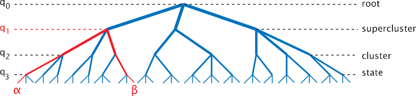
Figure 1: Taxonomic structure of the tree of states in a simplified example with $K=3$. Notice that the overlap between states $\alpha$ and $\beta$ is $q_{\alpha\beta}=q_{1}$.

The study of such a complicated phase is made manageable by the observation that the geometry of the space of equilibrium states is ultrametric and thus can be organized in a hierarchical tree [10, 12]. In order to understand what this means, let us consider a simplified example where $x(q)$ is discrete and the overlap can only take four different values $q_{0}<q_{1}<q_{2}<q_{3}$ (this is equivalent to the solution with $K=3$ RSB steps). We can see a schematic representation of such a tree in Figure 1. The ultrametric structure of the $q_{\alpha\beta}$ means that we can represent the spin-glass phase as a taxonomic tree of states, where the overlap between $\alpha$ and $\beta$ depends only on their closest common ancestor. The first consequence of this is that the self-overlap is state-independent,

$$q_{\alpha\alpha}=q_{\mathrm{M}},\qquad\forall\alpha.$$ (12)

A second consequence is that we can group the states in clusters (states with overlap $\geq q_{2}$) and superclusters (states with overlap $\geq q_{1}$).

Therefore, we can make the decomposition of Eq. (4) in terms of clusters $I$:

$$\langle O\rangle=\sum_{I}W_{I}\langle O\rangle_{I},\qquad W_{I}=\sum_{\alpha\in I}w_{\alpha}.$$ (13)

Of course, the real tree of states of a mean-field spin glass is more complicated than the representation in Figure 1: the real function $x(q)$ is continuous, so there are infinitely many overlap levels (the tree branches out at any value of $q$ from $q=0$ up to $q_{\alpha\alpha}=q_{\mathrm{M}}$) and, moreover, there are infinitely many branches at any level. Notice, however, that the ultrametric structure preserves the decomposition of (13), which now can be made arbitrarily for any value of $q$ (the only intrinsic decomposition being that at the state level, i.e., at $q=q_{\mathrm{M}}$).

In keeping with the tree metaphor, throughout the paper we shall also refer to the clusters of states at an arbitrary level $q$ (including their subclusters) as the ‘branches’ and to the states as the ‘leaves’.

The analytical study of this infinite tree was first performed by Mézard, Parisi and Virasoro (see [5]) and then formalized in terms of Ruelle’s probability cascades [13, 14, 15, 16, 17]. For instance, the probability distributions for the weights at any level $q$ can be written as [10]:

$$P(W;q)=\frac{W^{x(q)-1}(1-W)^{x(q)-1}}{\Gamma(1-x(q))\Gamma(x(q))}\ .$$ (14)

Notice how the sample-averaged function $x(q)$ controls the fluctuations. These weights have an immediate physical meaning, but they are cumbersome to handle, because they are not independent ($\sum_{I}W_{I}=1)$. However, we can obtain a simpler representation of the tree statistics by going back to the free-energy fluctuations, as defined in (6). Indeed, as it turns out, the $f_{\alpha}$ are independent variables [18]

$$\mathcal{P}(f_{\alpha})\propto\mathrm{e}^{-\beta x(q_{\mathrm{M}})f_{\alpha}}\;.$$ (15)

In fact, we can perform the analogous operation at any level of $q$:

$$W_{I}=\frac{\mathrm{e}^{-\beta f_{I}}}{\sum_{J}\mathrm{e}^{-\beta f_{J}}},\qquad\mathcal{P}_{q}(f)\propto\mathrm{e}^{-\beta x(q)f}.$$ (16)

Again, we see that this construction is universal, in the sense that everything is encoded in the function $x(q)$.

Our aim in this study is the explicit generation of trees of states for mean-field spin glasses. Naturally, since we cannot deal numerically with infinite trees, we will need to introduce two approximations:

1. Discretize the function $x(q)$. This is not a very delicate step as long as we keep the correct $x_{\mathrm{M}}=x(q_{\mathrm{M}})$: the branching levels are arbitrary and we just have to keep a sufficient number of branching steps to represent the $x(q)$ function faithfully. In keeping with the usual nomenclature, we shall occasionally refer to a tree with $K$ branching levels as a solution with $K$ RSB steps.

2. We have to prune the tree in order to have a finite number of states.

This second step seems dangerous, but it can be controlled quite easily [6]. In particular, it is easy to see that the total number of states with $w>p$ increases as $p^{-x_{\mathrm{M}}}$. Therefore, if we study the system with resolution $\epsilon$, neglecting all the states with $w<\epsilon$, we are losing a total probability of $\sim\epsilon^{1-x_{\mathrm{M}}}$. In the following section we describe how to generate an explicit realization of this pruned tree.

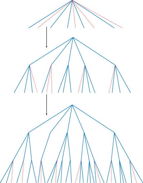
Figure 2: Schematic representation of the iterative generation of a pruned tree with $K=3$ RSB steps. At each step we generate new branches of the tree and discard all the branches (clusters of states) with weight $W_{I}$ smaller than a cutoff $\epsilon$ (represented with red dotted lines in the figure). The other branches are kept and used to generate new subclusters, which are in turn pruned. The process is iterated until we reach the highest value of the overlap, which defines the classification of the system in pure states. Since the weight of a state is always smaller than the weight of the branch that leads to it, this process is equivalent to discarding all the states with weight $w_{\alpha}<\epsilon$. The tree pruned in such a way will lose a total probability of $\sim\epsilon^{1-x_{\mathrm{M}}}$.

3 Generating the tree from the trunk down to the leaves

In the previous section we saw how one can achieve a mathematical description of the tree of states independently for any given level (i.e., at any value of $0\leq q\leq q_{\mathrm{M}}$). However, in this study we are not interested in the statistics of isolated levels of the tree, but in the explicit generation of its whole structure, i.e., the whole set of $\{w_{\alpha},q_{\alpha\beta}\}$. To this end, we shall construct an iterative representation of the tree, starting with the trunk and branching out step by step down to the individual states. At each step, we shall have a collection of clusters of states with weights $W_{I}$. We shall then discard all the clusters with weight $W_{I}<\epsilon$ (this is stricter than discarding all the states with $w_{\alpha}<\epsilon$) and then, for each cluster, generate its subclusters. At each step we shall keep the whole structure of the tree (i.e., the lists of ancestors for each subcluster). Figure 2 shows a schematic representation of such a pruned tree.

In this section we explain how such a construction can be attempted, starting with the simplest case where $q$ can only take two different values (one step of RSB) and then generalizing to $K$ RSB steps and to the continuous limit. Our algorithm is based on a description of the tree along the lines sketched in the previous section, see [19] for a different approach to the construction of random recursive trees.

3.1 One-Step RSB

Let us start by considering the construction of the pruned tree in the 1-RSB case, where the overlap can only take two values.

$$q(x)=q_{0}\ \mbox{for}\ x<m,\qquad q(x)=q_{1}\ \mbox{for}\ m<x\ ,$$ (17)

where it is assumed that the parameter $m$ is less that one and $q(x)$ is just the inverse of the function $x(q)$ of eq. (11). We have, then, a very simple tree

$$q_{\alpha,\alpha}=q_{1},\qquad q_{\alpha,\gamma}=q_{0}\ \ \mbox{for}\ \alpha\neq\gamma\ .$$ (18)

The weights can be constructed in the following way. Remembering (16), we consider a Poisson point process with a probability $\exp[\beta m(f-f_{0})]$. More precisely we extract numbers on the line where the probability of finding a point in the interval $[f:f+\mathrm{d}f]$ is given by

$$\mathrm{d}\rho_{m}(f)\equiv\exp\bigl{[}\beta m(f-f_{0})\bigr{]}\mathrm{d}f\,.$$ (19)

If we label these points with an index $\alpha$ we can set

$$w_{\alpha}=\frac{\exp(-\beta f_{\alpha})}{\sum_{\gamma}\exp(-\beta f_{\gamma})}\,.$$ (20)

The weights generated in this way have the correct probability distribution. A few comments are in order:

• The construction is consistent, i.e., $\sum_{\gamma}\exp(-\beta f_{\gamma})<\infty$ and $\sum_{\alpha}w_{\alpha}=1$.

• The distribution is stochastically stable: if we set $f^{\prime}_{\alpha}=f_{\alpha}+\delta f_{\alpha}$, where the $\delta f_{\alpha}$ are identically independent distributed variables, the probability distribution of the $f^{\prime}$ is the same (apart from a variation of $f_{0}$) and the probability distribution of the $w$’s does not change.

• If we prune the tree and we consider only the states such that $w_{\alpha}>\epsilon$, we have that $\sum_{\alpha}w_{\alpha}=1-O(\epsilon^{-\lambda})$ with $\lambda=1/m-1>0$.

• The parameters $f_{0}$ and $\beta$ are irrelevant from the numerical point of view. They are introduced only for later use and for the physical interpretation (remember Section 2).

• If we consider a process where the $f_{\alpha}$ are restricted in the interval $[-\infty,\Lambda]$ (which is simpler to generate numerically) the probability distribution of the $w_{\alpha}$ converges to the right one in the limit $\Lambda\to\infty$.

• The $w_{\alpha}$ can be easily generated numerically. One extracts $M$ numbers $r_{\alpha}$ with a a flat distribution in the interval $[0,1]$. Then we set $z_{\alpha}=1/r_{\alpha}^{1/m}$ and

  $$w_{\alpha}=\frac{z_{\alpha}}{\sum_{\gamma}z_{\gamma}}\,.$$ (21)

  The ratio of the largest to the smaller value of the $w$’s is of order $M$. The parameter $M$ (fixing the maximum number of descendants for each node) plays the same role as $\epsilon$ with

  $$\epsilon=O(M^{-\lambda})\,.$$ (22)

3.2 Two-Step and $K$-Step RSB: the naive method

Now consider a tree with two steps of RSB, that is, when $q(x)$ has two discontinuities. We have

$$q(x) = q_{0}\quad\mbox{for}\quad x<m_{1},$$ (23)

$$q(x) = q_{1}\quad\mbox{for}\quad x<m_{1}<x<m_{2},$$ (24)

$$q(x) = q_{2}\quad\mbox{for}\quad m_{2}<x.$$ (25)

In this case we can simply generalize the previous equations and we can label the states by a pair of indices $\alpha_{1}$ (cluster) and $\alpha_{2}$ (state within each cluster). We now have

$$q_{\alpha_{1}\alpha_{2};\gamma_{1}\gamma_{2}}=q_{0} + (q_{1}-q_{0})\delta_{\alpha_{1},\gamma_{2}}+(q_{2}-q_{1})\delta_{\alpha 1\alpha 2;\gamma_{1}\gamma_{2}}\,,$$

where $\delta_{\alpha 1\alpha 2;\gamma_{1}\gamma_{2}}$ is a shorthand notation for $\delta_{\alpha_{1},\gamma_{1}}\delta_{\alpha 2,\gamma_{2}}$.

The weights are given by

$$w_{\alpha,\gamma}=\frac{\exp(-\beta f_{\alpha,\gamma})}{\sum_{\alpha,\gamma}\exp(-\beta f_{\alpha,\gamma})}\,,$$ (26)

with

$$f_{\alpha_{1},\alpha_{2}}=g_{\alpha_{1}}+g_{\alpha_{1},\alpha_{2}}\,,$$ (27)

where the $g_{\alpha_{1}}$ are generated with a density $\rho_{m_{1}}(g)$ and the $g_{\alpha_{1},\alpha_{2}}$ are generated with a density $\rho_{m_{2}}(g)$.

The construction is quite simple and it can be generalized to any number of levels, adding a new term and a new index to the free energy at each step. However, the limit where the number $K$ of levels goes to infinity is mathematically complicated. In fact, the mere existence of such a limit (proved by Ruelle [13]) is non-trivial. It is already not evident in the two-step case that, in the limit where $m_{1}\to m_{2}$, the dependence on $q_{1}$ disappears and we recover the one-step formulae.

In any case, from a numerical point of view the most serious problem is that the number of random free energies goes as $M^{K}$, which rapidly explodes, even noticing that in the limit $K\to\infty$ we can take $M=2$.

To put it in another way, as discussed in Section 2 we can define the weight of a cluster $\alpha_{1}$ as the sum of the weights of all its states,

$$w_{\alpha_{1}}=\sum_{\alpha_{2}}w_{\alpha_{1},\alpha_{2}}.$$ (28)

But notice that now we cannot know the value of this weight just from the set of $g_{\alpha_{1}}$ without having also the $g_{\alpha_{1},\alpha_{2}}$: two clusters with the same value of $g_{\alpha_{1}}$ may end up with different weights at the end of the process and, therefore, we cannot discard any cluster until we have generated the whole tree down to the states. The states with the largest weight may not belong to the clusters with the lowest $g_{\alpha}$.

We need to find a different decomposition of the state free energy so that the relationship (26) can be applied at each step in the construction of the tree and the $g_{\alpha}$ for each cluster can be understood as a “cluster free energy” in the sense of (16).

3.3 $K$-Step RSB cluster by cluster

We present here an alternative way to generate the weights that does not suffer from these shortcomings. Let us consider a tree discretized for $K+1$ values of $q$, from $q_{0}$ to $q_{K}$. We start by generating all the clusters at level $q_{0}$ following equation (21), with $m=x(q_{0})$. This gives us a set of cluster weights $w_{\alpha_{1}}$. The next step is generating a set of weights $w_{\alpha_{1},\alpha_{2}}$ at level $q_{1}$, with the constraint that each $w_{\alpha_{1}}$ must be the sum of the weights of its subclusters. That is, we parameterize the $w_{\alpha_{1},\alpha_{2}}$ as

$$w_{\alpha_{1}\alpha_{2}}=w_{\alpha_{1}}t_{\alpha_{1},\alpha_{2}}\,,$$ (29)

where the $t_{\alpha_{1},\alpha_{2}}$ satisfy the constraint:

$$\sum_{\alpha_{2}}t_{\alpha_{1},\alpha_{2}}=1\,.$$ (30)

Finally, we write

$$t_{\alpha_{1},\alpha_{2}}={\exp(-g_{\alpha_{1},\alpha_{2}})\over\sum_{\alpha_{2}}\exp(-g_{\alpha_{1},\alpha_{2}})}\,.$$ (31)

Now the $g_{\alpha_{1},\alpha_{2}}$ have a slightly different interpretation to the ones in the previous section. The most important difference is that the new quantities are not independent, since they are constrained to belong to the same cluster $\alpha_{1}$.

The probability distribution of the $g_{\alpha_{1},\alpha_{2}}$ can be found in the literature, see eq. (14) in [18]:

$$\mathcal{P}_{\{g\}}\propto\biggl{(}\prod_{\alpha_{2}}\mathrm{d}\rho_{m_{2}}(g_{\alpha_{1},\alpha_{2}})\biggr{)}\biggl{(}\sum_{\alpha_{2}}\exp(-\beta g_{\alpha_{1},\alpha_{2}})\biggr{)}^{m_{1}}.$$ (32)

In this equation, we have defined $m_{1}=x(q_{0})$, $m_{2}=x(q_{1})$.

Let us now see how we can construct a numerical method to generate these $g_{\alpha_{1},\alpha_{2}}$ according to (32). The first step, as already discussed in Section 3.1 is to consider a maximum number $M$ of subclusters. Then, we order the $g_{\alpha_{1},\alpha_{2}}$ so that $g_{\alpha_{1},1}$ is the lowest and we rewrite (32) as

$$\mathcal{P}_{\{g\}}\propto\exp\biggl{[}-\beta(m_{2}-m_{1})g_{1}-\beta m_{2}\sum_{i=2}^{M}g_{i}\biggr{]}C(\{g\}),$$ (33)

where we have used a single index $i$ for the $g_{\alpha_{1},i}$ to lighten the notation and

$$C(\{g\})=\biggl{[}1+\sum_{i=2}^{M}\exp\bigl{(}-\beta(g_{i}-g_{1})\bigr{)}\biggr{]}^{m_{1}}.$$ (34)

In order to discuss this equation, let us first assume $C(\{g\})=1$ and let us define $\Delta=m_{2}-m_{1}$. We then find that the density of the $g_{i}$ for $i>1$ is cutoff at $-1/m_{2}$, while the density of $g_{1}$ has a cutoff at $-1/\Delta$. Therefore, for small $\Delta$ the quantity $g_{k}-g_{1}$ will be of order $1/\Delta$ aside from events that have probability $\Delta$.

Let us now discuss the delicate point of how to generate these $M$ values of $g_{i}$ in the correct way using a Monte-Carlo-like algorithm (i.e., through repeated random suggestions until one is accepted with a given probability).

We start by considering the case where we put $C(\{g\})=1$.

1. We generate the $M-1$ free energies for $i>1$ in the region $[-\infty,0]$ with a probability proportional to $\exp(m_{2}h)$.

2. We generate $g_{1}$ in the region $[-\infty,0]$ with a probability proportional to $\exp(\Delta g_{1})$.

3. We need that $g_{1}$ be the smallest one, i.e., $g_{1}\leq g_{k}\ \forall k$. If $g_{1}$ is not the smallest we go back to point 1 and we repeat until success.

In order to estimate the goodness of the algorithm we have to know the probability that the suggestion is accepted. The condition can be written also as $g_{1}\leq h^{*}$, where $h^{*}=\min_{k>1}g_{k}$. The probability of this event is $\exp(\Delta h^{*})$. Now, for large $M$ we have that $\exp(-m_{2}h^{*})=\mathcal{O}(M)$ (the minimum of $M$ variables does not fluctuate when $M$ goes to infinity). We conclude that the acceptance probability goes to zero as $M^{-\Delta/m_{2}}$, where $\Delta/m_{2}$ is less that one.

We have to take care now of the factor $C(\{g\})>1$. It is evident that $1<C(\{g\})<M^{m_{1}}$. We can thus interpret $C(\{g\})/M^{m_{1}}$ as a probability. Therefore, in order to take $C(\{g\})$ into account we only accept the suggestion of the previous three steps with a probability $C(\{g\})/M^{m_{1}}$. In this case the acceptance rate will be greater that $1/M^{m_{1}}$. The strategy works and there is a slowing factor of the algorithm due to the rejection that increases as a power of $M$ less that one.

In the limit $\Delta\to 0$, the average value of the acceptance of the first step goes to 1, the acceptance of the second one $1/M^{m_{1}}$ and the distribution becomes concentrated on the case where one of the $t_{\alpha_{1},\alpha_{2}}$ is one and the others are zero, thus recovering the 1RSB process.

Obviously, once we have the subclusters at level $q_{1}$ we can iterate the same construction until we reach level $q_{K}$.

This new algorithm is more complicated than the one in Section 3.2, but has the considerable advantage that now we can perform a preemptive pruning of the tree at each step to avoid the the explosion of terms in the limit $\Delta=(m_{2}-m_{1})\to 0$. We simply discard all the subclusters that have a weight less that $\epsilon$ (i.e., those with $\mathrm{e}^{-\beta g_{i}}/\sum_{j}\mathrm{e}^{-\beta g_{j}}<\epsilon$). In this way we eventually generate consistently all the states that have weight greater than $\epsilon$. At each step we are considering a fixed number $M$ of descendants, most of which will be pruned. In this way the complexity is of order

$$\mathcal{O}(M^{1+x^{*}}\Delta^{-1}\epsilon^{-\omega})\,,$$ (35)

and diverges only in a linear way when $\Delta$ goes to zero.

The error on the final results is also a monomial in the control parameters $M$, $\Delta$ and $\epsilon^{-1}$ (its precise form depends on the observables), so that we have reached our goal of generating the hierarchical tree in a polynomial time. However, there is still ample space for improvements, which will be described in A. At the end of the day the computational complexity can be reduced just to

$$\mathcal{O}(\epsilon^{-\omega})\,,$$ (36)

or, in other words, to the number of leaves, which is clearly the best achievable.

Finally, we must keep in mind that this method describes the generation of a single tree (sample). In order to obtain physically meaningful results we have to generate many trees in order to perform the average over the disorder.

4 The cavity equations and the iterative reweighting of the tree

So far we have seen how, starting from a known function $q(x)$ we can generate the complete tree of states, which in itself already gives us a lot of information on the spin-glass phase (see Section 6). In this section we show how to exploit this tree to compute more sophisticated physical quantities employing a cavity approach [20, 5, 21] and how we can use this cavity step in order to reweight the tree. This in principle allows us to compute the, initially unknown, correct $q(x)$.

Let us start from a nearly infinite system (of size $N$) with $K$ steps of RSB and let us add a new spin $\sigma_{0}$ to the system. We assume that connected correlation functions inside a state are negligible among generic points (cluster decomposition property). We define the effective magnetic field on the new spin in a state $\alpha$ as

$$h_{\alpha}=\sum_{k=1}^{N}J_{0,k}m_{k}^{\alpha}\,.$$ (37)

For later uses we assume that the $J_{0,k}$ are i.i.d. random variables with zero average and variance $1/N$.

Let us consider a given system of size $N$ with weight values $w_{\alpha}$ (that are ordered in a decreasing way). It is well known [5] that one can solve the model using the cavity approach where the properties of the system with $N+1$ variables are related to those of the system with $N$ variables through the following recursive relations

$$m_{0}^{\alpha} = \tanh(\beta h_{\alpha})\,,$$ (38)

$$h_{\alpha} = \sum_{k=1}^{N}J_{0,k}m_{k}^{\alpha}\,,$$ (39)

$$w^{\prime}_{\alpha} = w_{\alpha}\exp(-\beta\Delta f)\,,$$ (40)

$$\Delta f = -{\log(2\cosh(\beta h_{\alpha}))\over\beta},$$ (41)

where $m_{0}$ is the magnetization of the new spin, $w_{\alpha}$ and $w_{\alpha}^{\prime}$ are the unnormalized weights of state $\alpha$ respectively in the $N$ variables and $N+1$ variables systems. As usual, we are assuming a one-to-one correspondence between states for low energy in the two systems.

It is evident that the overlaps $q_{\alpha,\gamma}$ have changes only of order $1/N$. In principle, the probability distribution of the $w^{\prime}_{\alpha}$ might be different from the probability distribution of the $w_{\alpha}$. Moreover, the $w_{\alpha}$ depend on the $h_{\alpha}$, so that the $w^{\prime}_{\alpha}$ and the $h_{\alpha}$ may be correlated. However, this does not happen if we start from the previously presented distribution of the $w_{\alpha}$. In order to understand this, let us first notice that the $h_{\alpha}$ are random Gaussian variables with zero averages and covariances

$$\overline{h_{\alpha}h_{\gamma}}=q_{\alpha,\gamma}\,.$$ (42)

We do not need to know the values of the $m_{k}^{\alpha}$. The only information we need is

$$N^{-1}\sum_{k=1,N}m^{\alpha}_{k}m^{\gamma}_{k}=q_{\alpha,\gamma}\,.$$ (43)

It is worth noticing at this stage we can forget the value of $N$. Fortunately stochastic stability implies that the probability distribution of the $w^{\prime}_{\alpha}$ (ordered) is the same of that of the $w_{\alpha}$ and that the $h_{\alpha}$ are uncorrelated to the $w^{\prime}_{\alpha}$ [22].

We can now impose the self-consistent condition that if we take two states $\alpha$ and $\gamma$ that have overlap $q$, then the average overlap of the new spin will be also $q$:

$$\langle\tanh(\beta h_{\alpha})\tanh(\beta h_{\gamma})\rangle_{q_{\alpha,\gamma}=q}=q\,.$$ (44)

The result should not change if we add further conditions on the values of the $w_{\alpha}$.

We can now proceed in two different directions:

• We evaluate the l.h.s. of eq. (44) in an analytic way. In the case of a finite number of steps, we can write an explicit expression in terms of nested integrals [12] that collapses to the solution of a parabolic differential equation in the $K\to\infty$ limit.

• In the same way that it has been done [21] in the one-step (and sometimes in the two-step) RSB on the Bethe lattice we can impose equation (44) by evaluating the l.h.s. by generating both the trees and the $h_{\alpha}$ numerically and computing the average over different distributions.

Here we will follow this second approach. Our motivations are the following:

• We believe that such a cavity computation may be useful to understand the physical meaning of full RSB.

• This full RSB cavity computation may be a first step towards the full RSB cavity computation in the Bethe lattice, where a replica computation is not available.

• We plan to compute the loops corrections to mean field theory using the cavity approach. The computation of the loop expansion is a longstanding problem and in spite of the great progresses done in the replica approach, we do not know the infrared behavior of the one loop corrections. This long alternative cavity approach may be a viable tool to overcoming this difficulty.

Let us discuss the numerical implementation of the previous approach. We start by generating the $w_{\alpha}$ as discussed in Section 3. The generation of the $h_{\alpha}$, following (42), is trivial. We can extract a Gaussian random variable for each piece of the branch and add the different terms. That is, each state $\alpha$ will have an associated cavity field $h_{\alpha}$

$$h_{\alpha}=h_{\alpha}^{0}+h_{\alpha}^{1}+\ldots+h_{\alpha}^{K}.$$ (45)

The first term, $h_{\alpha}^{0}$ is actually common to the whole tree and is extracted from a Gaussian distribution with variance $\beta q_{0}$. Then each of the $h^{i}_{\alpha}$ is extracted from a Gaussian distribution with variance $\beta(q_{i}-q_{i-1})$ and is common to all the states along the same branch. The last piece, $h_{\alpha}^{K}$, is individual for each state.

The main problem comes from pruning, which is not stable to the reweighting. If the initial tree was pruned at a level $\epsilon$, this will not happen after the reweighting. Some of the $w^{\prime}_{\alpha}$ will be smaller than $\epsilon$ and some states in the region with $w^{\prime}_{\alpha}$ near to $\epsilon$ will be missing. Only the part of the tree that is far form the boundary (in a log scale) will remain accurate under the pruning.

At the end of the day we get the equation:

$${\sum_{\alpha,\gamma}\delta(q_{\alpha,\gamma}-q)G(w^{\prime}_{\alpha},w^{\prime}_{\gamma})\tanh(\beta m_{\alpha})\tanh(\beta m_{\gamma})\over\sum_{\alpha,\gamma}\delta(q_{\alpha,\gamma}-q)G(w^{\prime}_{\alpha},w^{\prime}_{\gamma})}=q$$ (46)

where $G(w^{\prime}_{\alpha},w^{\prime}_{\gamma})$ can be chosen arbitrarely. The simplest choice $G=1$ is however not good, because it is dominated by the many states of small weigth; in order to concentrate the measure on the high $w$ states we use

$$G(w^{\prime}_{\alpha},w^{\prime}_{\gamma})=w^{\prime}_{\alpha}w^{\prime}_{\gamma}\,,$$ (47)

but other different choices are possible. We also notice that a smoothing over the $q$ values is also necessary, since we cannot impose numerically a strict delta function.

The computation in the zero-temperature limit is quite similar:

$$m_{0}^{\alpha}=\mbox{sign}(h_{\alpha})\,,\ \ E^{\prime}_{\alpha}=E_{\alpha}-\mbox{abs}(h_{\alpha})\,,\ \ \overline{h_{\alpha}h_{\gamma}}=q_{\alpha,\gamma}\,.$$ (48)

The self-consistency equation becomes (with an appropriate choice of the function $G$):

$${\sum_{\alpha,\gamma}\delta(q_{\alpha,\gamma}-q)\exp\left(-\lambda(E^{\prime}_{\alpha}+E^{\prime}_{\gamma})\right)\mbox{sign}(h_{\alpha}h_{\gamma})\over\sum_{\alpha,\gamma}\delta(q_{\alpha,\gamma}-q)\exp\left(-\lambda(E^{\prime}_{\alpha}+E^{\prime}_{\gamma})\right)}=q\,.$$ (49)

In order for the previous equation to be dominated by the region where an accurate evaluation of the modified energies is available we must have that $\exp(-\lambda\Omega)$ should be very small. The value of $\lambda$ should be tuned as function of the details of the simulation and of the value of the cutoff energy $\Omega$; systematic errors decreases with increasing $\lambda$, but statistical errors increase, so a compromise is needed.

5 Testing the program

We have described how to generate the whole tree knowing $q(x)$. In Section 4 we also described how we can use a reweighting method to refine our values for the $q_{\alpha,\gamma}$ (and, thus, for the overlaps $q_{i}$ at the predefined branching levels $m_{i}$). In this section we test the consistency of this program. We check that the correct $q(x)$ for the chosen working temperature is stable and also that the tree it produces has the expected structure. Finally, we explore the dependence of the result on parameters such as $\epsilon$. Throughout this section, we use the large-$M$ modification of the program, as described in A.

Let us start by considering the model at $T=0.85$, close to the critical point $T_{\mathrm{c}}=1$. In these conditions, $q(x)$ is linear with very good approximation. This linearity simplifies matters because we only need two parameters to fix the whole $q(x)$ function: $q_{\mathrm{M}}=q_{K}$ and $x_{\mathrm{M}}=m_{K}=x(q_{\mathrm{M}})$. In order to calculate $q(x)$ from the trees, the steps would be

1. Find the correct $q_{\mathrm{M}}$ for a fixed $x_{\mathrm{M}}$ (i.e., the fixed point for the iterative method described in Section 4) and compute the free energy $F(x_{\mathrm{M}})$.

2. Minimize $F(x_{\mathrm{M}})$ to find the correct $x_{\mathrm{M}}$.

The first step is the more interesting one, since it will let us explore the properties of the numerical tree and its dependence on the parameters $K$ and $\epsilon$. Therefore, in the following we are going to work with the known $x_{\mathrm{M}}\approx 0.233122$ (this value has been computed with a Padè resummation technique and is accurate to six significant figures [4, 23]).

5.1 Computing $q_{\mathrm{M}}$

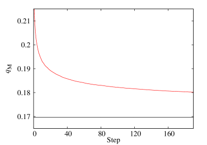
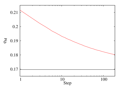
Figure 3: Evolution of $q_{\mathrm{M}}^{(t)}$ along the iterative reweighting of the tree at $T=0.85$, starting with $q_{\mathrm{M}}^{(0)}=x_{\mathrm{M}}$ in a linear (top) and a logarithmic (bottom) scale. We use $K=20$, $\epsilon=10^{-5}$ and $x_{\mathrm{M}}=0.233122$ [4]. The approach to the correct value $q_{\mathrm{M}}\approx 0.169691$ (horizontal line) is very slow.

For this first example, we are going to work with $\epsilon=10^{-5}$, so we are going to keep $1-\epsilon^{1-x_{\mathrm{M}}}\approx 99.99\%$ of the probability. Also, since $q(x)$ is linear, a relatively small value of $K=20$ should be sufficient. In the next sections we shall examine the effect of varying these parameters.

We are going to denote by $q_{i}^{(t)}$ the value of $q_{i}$ at iteration $t$. In order to kick off the computation we start with $q_{\mathrm{M}}^{(0)}=x_{\mathrm{M}}$. In each iteration we generate and average over $10^{6}$ trees (with the parameters described above, this takes only about 2 min per iteration on a single CPU). The result for $q_{\mathrm{M}}^{(t)}$ can is shown in Figure 3.

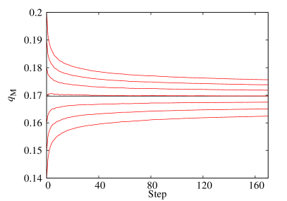
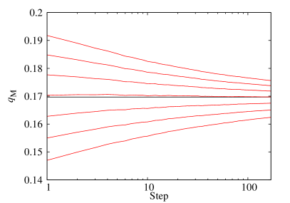
Figure 4: As in Figure 3, but now we consider several values of $q_{\mathrm{M}}^{(0)}$ to try to find the stable one (we use, from bottom to top, $q_{\mathrm{M}}^{(0)}=0.14,0.15,\ldots,0.20$). A few steps are enough to know whether our $q_{\mathrm{M}}^{(0)}$ is above or below the correct one. Once we find a good $q_{\mathrm{M}}^{(0)}$, convergence is very fast: with $q_{\mathrm{M}}^{(0)}=0.17$ we obtain $q_{\mathrm{M}}^{(200)}=0.1696(3)$, to be compared to $q_{\mathrm{M}}\approx 0.169691$ [4].

From the figure, we can see right away that this is not a workable method: the convergence of $q_{\mathrm{M}}^{(t)}$ is very slow (logarithmic). At the same time, the monotonic behavior of $q_{\mathrm{M}}^{(t)}$ suggests an alternative approach: start several simulations with different values of $q_{\mathrm{M}}^{(0)}$ and find the stable one. We have followed this method in Figure 4. We show several simulations, with values of $q_{\mathrm{M}}^{(0)}$ in increments of $0.01$. In each case, we have taken $200$ steps, although clearly only a few are necessary to know whether we are above or below the stable $q_{\mathrm{M}}$.

This new approach does work: with an (easy to find) good starting value of $q_{\mathrm{M}}^{(0)}=0.17$ we obtain $q_{\mathrm{M}}^{(200)}=0.1696(3)$, remarkably close to the exact value of $q_{\mathrm{M}}\approx 0.169691$ (see Fig. 4). Finally, although we have concentrated on $q_{\mathrm{M}}$, the whole $q(x)$ converges to the right one.

5.2 Consistency of the internal structure of the tree: the replicon propagator

We have seen that the reweighting method is able to find the correct $q(x)$. We still have to test whether this $q(x)$, in turn, generates a tree with the properties expected in the RSB theory. To this end, we consider the computation of the spin-glass susceptibility [5]

$$\chi_{\mathrm{SG}}=\frac{\overline{(1-m_{0}^{2})^{2}}}{1-\beta^{2}\overline{(1-m_{0}^{2})^{2}}}\ .$$ (50)

This quantity diverges for $T<T_{\mathrm{c}}$ so, in the denominator,

$$X=\beta^{2}\overline{(1-m_{0}^{2})^{2}}=1.$$ (51)

In terms of the trees, this equation can be written as

$$X=\beta^{2}\overline{\sum_{\alpha}w_{\alpha}(1-m_{\alpha}^{2})^{2}}=1,$$ (52)

where $m_{\alpha}$ has been defined in Section 4 and we remind the reader that the disorder average translates into an average over different realizations of the tree.

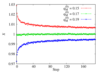
Figure 5: Value of $X^{(t)}$, defined in (52), which must be $X=1$ if the spin-glass susceptibility (50) is to diverge. Starting with $q_{\mathrm{M}}^{(0)}=0.17$ we obtain $X^{(200)}=0.9999(6)$.

We can see the evolution of $X$ for three different values of $q_{\mathrm{M}}^{(0)}$ in Figure 5. For $q_{\mathrm{M}}^{(0)}=0.17$ we obtain $X^{(200)}=0.9999(6)$, which is remarkably precise given the complicated structure of (52).

5.3 The dependence on $\epsilon$ and $K$

We have seen that the numerical method described in this paper is able to generate stable trees with the correct structure. Thus far, we have worked with fixed values of $K=20$ and $\epsilon=10^{-5}$ for the numerical parameters that determine the degree of discretization of the tree and the extent of its pruning, respectively. In this section we examine the effect of varying these quantities.

Let us start by considering the dependence on $K$, the number of RSB steps (or of different values of $q$). We have carried out simulations for $K$ ranging from $K=2$ to $K=20$. In each case, we have used $q_{\mathrm{M}}^{(0)}=0.17$ as our starting value and we have performed 200 reweighting steps, to ensure that the final values are stable. We report in Table 1 the resulting estimates for $q_{\mathrm{M}}$ and $X$ (the latter are also plotted in Figure 6). As we can see, the convergence to the right values is very smooth in $K$ and can be controlled. In particular, it is clear that the value $K=20$ that we have been using thus far is more than adequate.

Table 1: Evolution of our numerical estimates for $q_{\mathrm{M}}$ and $X$ with the number $K$ of RSB steps, starting with $q_{\mathrm{M}}^{(0)}=0.17$. For $K\gtrsim 12$, the values are compatible with the correct ones and the evolution is smooth (see also Figure 6).

• $K$	$q_{\mathrm{M}}^{(200)}$	$X^{(200)}$
  2	0.16487(9)	1.0101(7)
  4	0.16696(14)	1.0049(7)
  8	0.1685(3)	1.0020(7)
  12	0.1694(3)	1.0009(7)
  16	0.1688(6)	1.0007(7)
  20	0.1696(3)	0.9999(6)
  $\infty$	$0.169691\ldots$	$1$

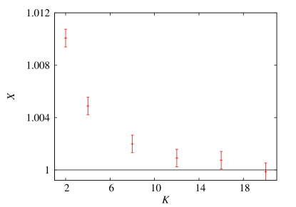
Figure 6: Evolution of our estimate for $X$ with the numbre $K$ of RSB steps, starting with $q_{\mathrm{M}}^{(0)}$. We take 200 reweighting steps, after which the estimate of $q(x)$ is stable. The value converges smoothly and quickly to the expectation $X=1$.

Table 2: Evolution of our numerical estimates for $q_{\mathrm{M}}$ and $X$ with the pruning parameter $\epsilon$, starting with $q_{\mathrm{M}}^{(0)}=0.17$. For $\epsilon\lesssim 10^{-3}$, the values are compatible with the correct ones.

• $\epsilon$	$q_{\mathrm{M}}^{(200)}$	$X^{(200)}$
  $10^{-1}$	0.1668(5)	1.0047(6)
  $10^{-2}$	0.1682(4)	1.0011(6)
  $10^{-3}$	0.1696(3)	0.9990(6)
  $10^{-4}$	0.1689(5)	1.0005(6)
  $10^{-5}$	0.1696(3)	0.9999(6)
  $0$	$0.169691\ldots$	$1$

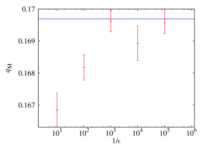
Figure 7: Evolution of our estimate for $q_{\mathrm{M}}$ with the pruning factor $\epsilon$, starting with $q_{\mathrm{M}}^{(0)}$. We take 200 reweighting steps, after which the estimate of $q(x)$ is stable. The value converges to the correct one (horizontal line) for moderate values of this parameter.

In Table 2 and Figure 7 we report the same quantities for simulations with different values of $\epsilon$. As we can see, even relatively coarse prunings produce rather accurate trees.

In summary, the dependence of the algorithm’s accuracy on the numerical parameters $\epsilon$ and $K$ is smooth and could be controlled in an eventual computation where the correct $q(x)$ were unknown.

6 An example application: peak counting and finite-size effects

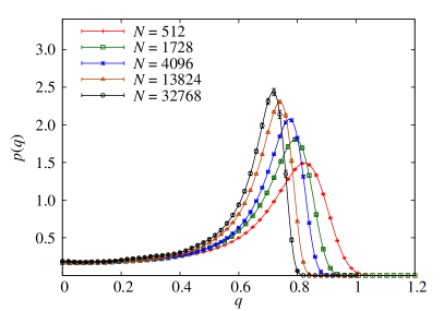
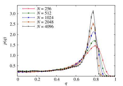
Figure 8: Comparison of the probability density of the order parameter $p(q)$ for the Sherrington-Kirkpatrick (data from [24]) and the Edwards-Anderson (data from [25]) models. Since the critical parameters of the two systems are different, we choose temperatures such that the $x(q)$ are similar for small $q$ ($T=0.4$ for SK and $T=0.7$ for EA).

We have a consistent method to generate the tree of states. In the previous section we have seen how it can be used to compute $q(x)$ for the SK model in a self-consistent manner. However, this is not our ultimate goal (there already are good methods to achieve this). Instead, we would like to use the detailed information contained in the tree to deepen our understanding of the spin-glass phase. In this section we give an example of a simple application with physical relevance.

We have been working from the outset with the mean-field Sherrington-Kirkpatrick model. It has been a longstanding debate in the community whether the $D=3$ version of the model (the Edwards-Anderson spin glass) has a similar behavior. The Edwards-Anderson spin glass is defined in a similar way as (1),

$$\mathcal{H}=-\sum_{\langle i,j\rangle}\sigma_{i}J_{ij}\sigma_{j},\quad\sigma_{i}=\pm 1,$$ (53)

but now the interaction are only between nearest neighbors (as denoted by the angle brackets in the sum) and the $J_{ij}$ are $\pm 1$ with $50\%$ probability.

Like the SK model, the EA spin glass system experiences a second-order phase transition [26, 27, 28], in this case at temperature $T_{\mathrm{c}}=1.1019(29)$ [29]. However, the details of its low-temperature phase are still disputed. In particular, a basic question is whether the $p(q)$ in $D=3$ is still non-trivial, as in the RSB picture, or whether there is only one state with $q=q_{\mathrm{M}}$, so the $p(q)$ is reduced to a single delta, as proposed by the droplet picture [30, 31, 32, 33].

Thus far, most numerical simulations (see, e.g., [25] for a detailed investigation) seem to point to the first option. We can see an example of this in Figure 8: both for the EA and SK cases, the value of $p(q=0)$ does not seem to evolve with the system size. For EA we use data generated with the Janus computer [34, 35] in [25]. For SK we use data from the simulations reported in [24, 36].

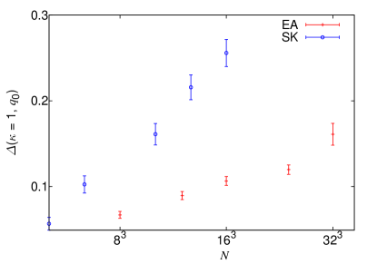
Figure 9: Evolution of $\Delta$ with the system size $N$ for the EA ($T=0.7$) and SK ($T=0.4$) models.

However, it has been argued that this approach is too naive, because the $p(q)$ may be in a preasymptotic regime (as suggested by the strong evolution of the peak) . As a consequence, several recent works have taken a more detailed approach, based on the study of the single-sample $p_{J}(q)$ [39, 40, 41, 42, 43, 44].

In particular, Yucesoy et al. [40] propose studying the following quantity

$$\Delta(q_{0},\kappa)=\mathrm{Prob}\bigl{[}\max_{q<q_{0}}\{p_{J}(q)\}>\kappa\bigr{]}.$$ (54)

As we have seen in Section 2, $\Delta\to 1$ when $N\to\infty$ for any finite $q_{0}$ in the SK model (because there are always states with $q<q_{0}$), while for a droplet system $\Delta$ should go to zero for large system sizes. If we represent this quantity (Figure 9) we can see that $\Delta$ grows much more slowly with $N$ in the EA model than in the SK one (even though it does not seem to go to zero, as predicted by the droplet model). Unfortunately, the larger statistical error in the largest size available for EA, $N=32^{3}$, makes it difficult to draw any direct conclusion from this figure. Since, as we saw in section 2, the sample-averaged $p(q)$ controls the statistics of the fluctuations, we have compared the two systems for temperatures where the $x(q)$ are similar (see Figure 8).

It has been proposed in [45] that the reason for the slower growth of $\Delta$ in EA is simply the slower evolution of the main peak, $p(q_{\mathrm{M}})$, in this system. Indeed, $p(q_{\mathrm{M}})\sim N^{\lambda}$ with $\lambda=1/3$ for SK but $\lambda\approx 0.1$ for EA [25] (the slower growth of the peak for EA can be seen graphically in Figure 8). Now, if the individual peaks in the $p_{J}(q)$ grew at the same rate, this would explain the apparent different behavior of $\Delta$ in the two models. We can use the numerical trees to explore this suggestion in detail.

Let us go back and consider the expression of $p_{J}(q)$ in terms of the trees (in the thermodynamical limit)

$$p_{J}(q)=\sum_{\alpha,\beta}w_{\alpha}w_{\beta}\ \delta(q-q_{\alpha\beta})=\sum_{A}P_{A}\ \delta(q-q_{A}),$$ (55)

where the lack of a disorder average signifies that we are considering a single realization of the tree (which would translate into a single sample in a more physical language).

Now, we can introduce a very simple model for the finite-size evolution of this $p_{J}$. We are going to consider that, for finite $N$, the delta functions are smoothed to have a finite width $W(N)$, independent of $q$ (a similar approach was followed in [46, 39] in a slightly different context). In addition, their position is shifted as

$$q_{A}^{(N)}=q_{A}^{\infty}+\eta,$$ (56)

where $\eta$ is a Gaussian random variable with standard deviation $W(N)$.

The value of $W(N)$ should go to zero as a power of $N$

$$W(N)=\mathcal{A}N^{-\zeta},$$ (57)

where $\mathcal{A}$ is a constant.

Now, since we are assuming that $W(N)$ is independent of $q$, we can use the self-averaging peak at $q=q_{\mathrm{M}}$ to fix $\zeta$ and $\mathcal{A}$. We see immediately that $\zeta=\lambda$, since $p(q_{\mathrm{M}},N)W(N)$ should be constant for large $N$. In order to fix $A$ we only need to consider (55)

$$p(q_{\mathrm{M}},N)=\frac{P_{M}}{\sqrt{2\pi}W(N)}=\frac{P_{M}}{\sqrt{2\pi}\mathcal{A}}N^{1/3}\,,$$ (58)

where $P_{M}$ is the weight of the delta function at $q=q_{\mathrm{M}}$ (so $P_{\mathrm{M}}=1-x_{\mathrm{M}}$ in the notation we have used in previous sections). We can know $P_{\mathrm{M}}$ from the exact solution in the thermodynamical limit and we can get $\mathcal{A}$ from a fit to numerical data for finite $N$. For $T=0.4$ the values are $P_{\mathrm{M}}\approx 0.49$ [4] and $\mathcal{A}\approx 0.91$ (from a fit to the data in [24]).

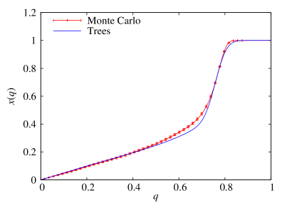
Figure 10: Sample-averaged probability density $P(q,N=4096)$ and cumulative probability $x(q,N=4096)$ for the SK model at $T=0.4$. We show the result of a Monte Carlo simulation at finite $N$ together with the ‘synthetic’ functions generated from the smoothed trees (the latter have much smaller statistical errors, which we do not show in the figure). Using the very simple smoothing procedure described in this section, we obtain a very accurate $x(q,N)$ for small $q$.

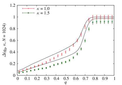
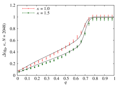
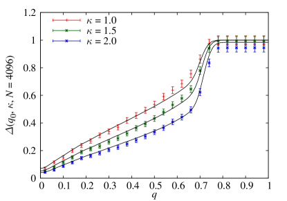
Figure 11: $\Delta(q_{0},\kappa,N)$ as a function of $q_{0}$ for several values of $\kappa$ and $N=1024,2048,4096$ at $T=0.4$. For $N=4096$ we include the results for $\kappa=1.0,1.5,2.0$. For the smaller sizes we do not include the last value, since the value of $p(q_{\mathrm{M}},N)$ in that case would be too small and, therefore, even for $q_{0}=1$ we $\Delta<1$, which is clearly a preasymptotic effect. For large system size, the $\Delta$ generated from the trees is very accurate. As in Figure 10, the statistical errors in the curves computed from the trees are one order of magnitude smaller.

With this information, we are in a position to generate ‘synthetic’ $p_{J}(q)$ for finite $N$ from our numerical trees. In particular, we take the following steps

1. Input the exact solution for $q(x)$ at $T=0.4$ from [4], and generate $\mathcal{N}$ trees. There is no need to consider the reweighting iterations, since we are already starting from the correct $q(x)$.

2. For each tree, knowing the values of $w_{\alpha}$ and $q_{\alpha\beta}$, we can construct the corresponding $p_{J}$ in the thermodynamical limit with (55).

3. For each tree, construct the finite-$N$ version of $p_{J}$ using $W(N)=0.91N^{-1/3}$, as obtained above.

Since we are only interested in relatively big peaks and $P_{A}\sim\mathcal{O}(w_{\alpha}^{2})$, a relatively coarse pruning suffices (we use $\epsilon=10^{-3}$, we have checked that $\epsilon=10^{-2}$ would have yielded compatible results). Since now the $q(x)$ is not linear, we need a finer discretization, so we use $K=100$. We generate $\mathcal{N}=10^{5}$ trees.

Notice that when generating the finite-$N$ $p_{J}$ the only adjustable parameters are $\lambda$ and $\mathcal{A}$, which we have fixed a priori.

Let us now look at the numerical results. In order to test our smoothing procedure, we are first going to check whether the average of the smoothed $p_{J}(q,N)$ reproduces the sample-averaged $p(q,N)$ computed in Monte Carlo simulations. We show the result for our largest available system, $N=4096$, in Figure 10. As we can see, the $P(q,N)$ is remarkably accurate for small $q$, even if it deviates close to $q_{\mathrm{M}}$ (this was to be expected, in particular our simple smoothing model does not represent well the shift in the peak’s position with growing $N$). More interestingly, the cumulative probability $x(q)$ is very accurate (this is a better-behaved function, which avoids the singularity at $q=q_{\mathrm{M}}$).

We are finally in a position to generate $\Delta(q_{0},\kappa,N)$ from the trees. The result for $N=1024,2048$ and $4096$ is shown in Figure 11. As we can see, for the larger system size the agreement between the ‘synthetic’ $\Delta$ generated from the trees and the one computed in MC simulations is excellent for a wide range of $\kappa$. The agreement is not as good for the smaller $N$, which was to be expected.

This analysis already explains the slower growth of $\Delta$ in EA compared to SK, simply because $\lambda=1/3$ for the latter and $\lambda=0.1$ for the former. Reference [45] goes a little farther and attempts to introduce a scaling ansatz for $\Delta$ that could be used to compare the results in EA and SK.

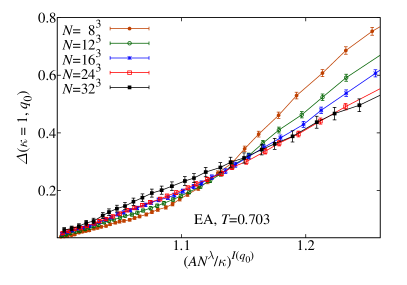
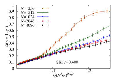
Figure 12: Scaling of $\Delta$ for EA and SK (results from [45]).

Indeed, $\Delta(\kappa,q_{0},N)$ is just the probability of finding a peak with weight $P_{A}>\kappa W(N)/\sqrt{2\pi}$. In the (very rough) assumption that there is only one relevant peak in $q<q_{0}$, we can integrate in (14) to estimate

$$\Delta(\kappa,q_{0})\propto[\kappa W(N)/\sqrt{2\pi}]^{-x(q_{0})}=[\mathcal{A}N^{\lambda}/\kappa]^{-x(q_{0})}.$$ (59)

This is a very simplified scaling, but could be used to compare EA and SK on equal grounds. In particular, for EA, as for SK, we could estimate $\mathcal{A}$ from the scaling of $P(q_{\mathrm{M}},N)$, as in (58). Unfortunately, for EA we do not know the value of $P_{\mathrm{M}}$, so the best we can do is assume that $P_{\mathrm{M}}^{\mathrm{EA}}\approx P_{\mathrm{M}}^{\mathrm{SK}}$. In [45] it was found that this scaling works reasonably well for the range of simulated system sizes (we reproduce the result of [45] in Figure 12).

The investigation of this scaling in [45] was limited to the range of $N$ accessible to MC simulation. However, with the trees we have in principle access to much higher values of $N$. In Figure 13 we show the same scaling plot including both MC data up to $N=4096$ and the results from the smoothed trees up to $N=262144$ . As we can see, the more precise results of the trees show that the scaling of (59), while a good first approximation, reveals its flaws once more data are considered.

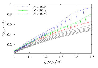
Figure 13: Scaling of $\Delta$ for SK using both Monte Carlo data (for $N=1024,2048$ and $4096$) and the smoothed trees (continuous lines, for values of $N$ growing from top to bottom in geometric progression: $N=1024,2048,\ldots,262\,144$). As we saw in Figure 11, the values of $\Delta$ for $N=2048,4096$ obtained in Monte Carlo simulation coincide with those from the trees. The larger system sizes achievable with the tree computation reveal the limitations of the scaling in (59).

We finally note that [47] pointed out that the scaling suggested in [45] failed once the temperature was changed. This is probably because [45] failed to take into account the factor $P_{\mathrm{M}}$ in (58), which is obviously temperature-dependent. In any case, it is clear that the scaling of $\Delta$ is quite complicated and a more detailed study (or larger numerical simulations) is needed to draw any quantitative conclusions from it. On a more qualitative level, however, the assumption that the main difference between SK and EA is due to the slower growth of the sample-averaged $p(q)$ in the latter seems well justified.

7 Conclusions

We have presented an efficient algorithm for the generation of the tree of states in mean-field spin glasses, once the $q(x)$ is given. Complemented with the cavity method this algorithm can also determine self-consistently the correct $q(x)$, although the convergence to such a solution seems to be rather slow.

The generation of many different tree of states, one for each sample, allows one to study analytically sample-to-sample fluctuations in mean-field spin glasses. As an application, we have studied the problem of peak counting in single-sample $p_{J}(q)$, showing that our analytical results coincide with Monte Carlo measurements in the SK model.

The method presented herein has potential to permit cavity computations in cases where the replica approach has not been fully successful, for instance, in the computation of loop corrections to the mean-field theory.

Appendix A Direct generation of the continuum tree

Here we will discuss some tricks that can be used to improve the speed of the algorithm in the limit of small $\Delta$. The approach of the previous sections was to consider the case where replica symmetry was broken at $K$ steps. Although we are interested to study the limit where $K$ goes to infinity, an algorithm that takes a linear time in $K$ is rather good, indeed many of the artifacts due to a finite value of $K$ go to zero as $1/K^{2}$ when $K\to\infty$. However, here we would like to discuss how to construct an algorithm that works directly in the limit $K\to\infty$. We have not used this algorithm in the numerical computations of this paper, because we do not need it for our aims, however we would like to present it, both for its elegance and for using it in future applications.

For the convenience of the reader we shall see how to obtain the new algorithm by subsequent improvements of the one presented in the main text. As we have done before, we first discuss the improvements in the case where the weighting factor is $C(\{g\})=1$ and later on we see how to keep track of the presence of this factor.

A.1 The limit $M\to\infty$

We have seen that the first phase of the algorithm consists in generating $M-1$ free energies $g_{i}$. We then evaluated their minimum and performed an acceptance test on it (which is nearly always accepted) in order to generate the $t_{i}$. We finally had to discard many of them (apart from the largest ones) because they violated the inequality $t>\epsilon$ and they would be eventually pruned.

It would certainly be better to generate directly the lowest free energies in order in the interval $[-\infty,+\infty]$, in such a way that we do not need to generate quantities that we do not use. Indeed, in the limit where $M$ goes to infinity the distribution probability of the $g_{i}$ becomes proportional to $\exp(-m_{2}g_{i})$. The proportionality factor ($\mathcal{O}(M)$) is irrelevant, since it may absorbed in a shift of the $g_{i}$. We can thus generate the $g_{i}$ from a Poisson process with density $\exp(-m_{2}g_{i})$. This result is particularly handy because it is easy to extract directly ordered variables generated with a Poisson process. In this way we obtain Gumbel type distributions.

Looking back at the formulae of the main text, we can use the well know result (that can be easily proved) that the ordered $g_{k}$ ($k=2...\infty$) can be directly generated in the following way. If we denote by $r_{k}$ random independent random numbers, equidistributed in the interval $[0,1]$, the $g_{k}$ can be obtained as

$$m_{2}g_{k}=\log(-\sum_{s=2,k}\log(r_{s}))\ ,$$ (60)

Let us consider the distribution of $g_{2}$. In principle its probability distribution can reach down to $-\infty$. However, it is strongly cutoff at large negative values. More precisely, a random number generator on a computer has minimum value $r_{m}$ ($r_{m}=2^{-32}$ for a typical 32-bit generator and $r_{m}=2^{-64}$ for a typical 64-bit generator). It is evident that

$$g_{2}>G\equiv\log(-\log(r_{m}))\ .$$ (61)

The constant $G$ is not large: for typical random generators $G\approx-3$ (32 bits) and $G\approx-4$ (64 bits).

Now we reproduce the probability distribution of the main text by going through the following steps:

• We propose a value of $g_{2}$ according to the previous distribution, i.e., $x_{2}g_{k}=\log(-\log(r_{2}))$.

• We accept the proposed value for $g_{2}$ with probability $\exp(\Delta(G-g_{2}))$. The probability is less than 1 by construction (as it should be). For small $\Delta$ it is also very near to 1 in most of the cases, so that the acceptance factor is near 1. We repeat this construction up to the moment that a value of $g_{2}$ is accepted.

• Once we have generated $g_{2}$ in this way, we finally set

  $$g_{1}=g_{2}+\log(r_{1})/\Delta\,.$$ (62)

• If $\exp(-(g_{2}-g_{1}))<\epsilon$ (this happens with probability $(1-\Delta)$) we stop and no branching happens at this level. On the contrary if $\exp(-(g_{2}-g_{1})>\epsilon$, a branch is present. We generate the other $g_{k}$ and stop as soon as $\exp(-(g_{k}-g_{1}))<\epsilon$. The average number of accepted $g_{k}$ is of order $-\log(\epsilon)/x_{2}$.

One can prove that this construction is equivalent to the one considered in the main text. It has the advantage that the computation can be done directly in the limit $M\to\infty$.

We now have to cope with the factor $C(\{g\})$. We have to accept the proposed branching with a probability that is proportional to $C(\{g\})$ and if the proposed branching is not accepted we have to go through the previous procedure again.

In principle the values of $C(\{g\})$ may be very large, but its probability is strongly cutoff at large values. In the real simulations, as far as a very large value of $C(\{g\})$ is very unlikely, we can accept the proposed configuration with a probability given by $C(\{g\})/C_{\mathrm{upper}}$, where $C_{\mathrm{upper}}$ is greater that the maximum value of $C(\{g\})$ in the simulation. The value of $C_{\mathrm{upper}}$ depends on the details of the simulation and it can be found by trial and error. In this way we can dispose of the parameter $M$.

A.2 The limit $K\to\infty$

We are now in the situation where we can consider directly the limit $K\to\infty$, by avoiding to do computations in the case where the proposed change is rejected.

Let us first consider the case where $C(\{g\})=1$ We notice that at a given level there can be bifurcations (or higher-order branching) in the tree only if the condition $\exp(-g_{2}+g_{1})>\epsilon$ is satisfied. This happens with probability $-\Delta\log(\epsilon)$. Therefore in the limit where $\Delta\to 0$ the distance $\delta x$ of the values of $x$ where we have a branching on the tree is an exponentially distributed random variable with average $-\log(\epsilon)$.

In this way we can directly compute the position of the next branching, extract the value of $g_{1}-g_{0}$ from a flat distribution in the interval $[0:-\log(\epsilon)]$ and proceed as before. In this way we generate the tree directly in the continuous limit where $\Delta=0$. The final algorithm depends only on the parameter $\epsilon$, which has a clear physical meaning.

We now have to cope with the factor $C(\{g\})$. There are two possibilities.

• We could proceed as before: we accept the proposed branching with a probability that is proportional to $C(\{g\})$, i.e., $C(\{g\})/C_{\mathrm{upper}}$.

• We simply forget the factor $C(\{g\})$ in the generation of the tree. In the computation of the observable we have to introduce an additional factor when we average over the trees. For any given tree $\cal{T}$, we define a probability $P(\cal{T})$ that is the product of all the $C(\{g\})$ computed at the branches of the tree. We also have to consider this additional factor when we compute the value of an observable. In other words, if the algorithm produces a sequence of trees ${\cal T}_{i}$ for $i=1,N$, the expectation value of a quantity $A(\cal{T})$ is given

  $$\langle A\rangle={\sum_{i=1,N}P({\cal T}_{i})A({\cal T}_{i})\over\sum_{i=1,N}P({\cal T}_{i})}$$ (63)

  The quantity $P({\cal T})$ fluctuates from one tree to another but it should remain of $\mathcal{O}(1)$, so that this second approach should be viable.

We notice that in the region where $x_{\mathrm{M}}$ is small the quantity $C(\{g\})$ becomes equal to 1 plus corrections in $x_{\mathrm{M}}$. In the Sherrington Kirkpatrick model this happens near the critical temperature. For similar reasons, in the low-temperature region $C(\{g\})$ becomes equal to 1 plus corrections proportional to the temperature. The quantity $P({\cal T})$ is the product of a finite number of terms so it also becomes equal to one in this limit.

A.3 The zero-temperature limit

It may be interesting to consider the zero-temperature limit of the previous construction. The function $\beta x(q,\beta)$ usually has a limit when $q$ goes to zero. We can thus define

$$y(q)=\lim_{\beta\to\infty}\beta x(q,\beta)\,.$$ (64)

In the SK model $y(q)$ behaves qualitatively as $q(1-q)^{-1/2}$. The quantities $g_{i}$ have the meaning of free-energy differences multiplied by a factor $\beta$ and therefore they are expected to be proportional to $\beta$. If we write $h=\beta f$, we have that $xh=yf$. In the zero-temperature limit free-energy differences become energy differences, so that the rescaled $h$ are themselves energy differences.

Let us discuss the construction of the tree in the region of $q<q^{*}$ in such a way that the maximum value of $y$ ($y^{*}$) is finite. Our aim it to reconstruct the energy of the low-energy states in the zero-temperature limit, if they are observed with resolution $q$. In order to make the whole computation possible we consider only states that have a finite energy difference from the ground state. At the end of the day we obtain the same formula as before after the rescaling.

When we prune the tree at low temperature, the value $\epsilon=\exp(-\beta\Omega)$ corresponds to considering only the states that have an energy $E_{\alpha}<\Omega$ (in order to simplify the notation we set the ground state energy to zero, i.e., all the energies are energy differences with the ground state). The total number of leaves is of order $\exp(y^{*}\Omega)$. It is evident that the computation becomes very long for large values of $y^{*}$ or $\Omega$.

Fortunately, in the zero-temperature limit the annoying factor $C(\{g\})$ becomes equal to 1 with probability 1. Indeed, not only is the exponent in the definition of $C(\{g\})$ small, but also the terms $\exp(-\beta(E_{k}-E_{1}))$ are exponentially small with probability 1. The possibility of neglecting $C(\{g\})$ is a great simplification. The final rules are rather simple and they are exposed below.

• The root of the tree has $E=0$ and $y=0$.

• If we start from a branching point with energy $E$ and level $y$ (or from the root), the probability distribution of the level of the next branching ($y_{\mathrm{next}}$) is given by

  $$D\exp(-(y_{\mathrm{next}}-y)/D)\,,$$ (65)

  where $D=\Omega-E$. If we find that for $y_{\mathrm{next}}>y^{*}$ no branching is present.

• The energies of the branches after the branching will be

  $$E_{1}=E\ \ \ E_{2}=E+(\Omega-E)r_{1}\ \ \$$ (66)

  $$E_{k}=E_{2}+\ {\log(-\sum_{s=2,k}\log(r_{s})))\over y_{next}}.$$

  While it is obvious that $E_{1}<\Omega$ with probability one, we will keep the $E_{k}$ with $k>1$ only if they satisfy the relation $E_{k}<\Omega$.

As in Sec. 3, this explains the generation of the tree from a known $y(q)$. The reweighting (and refining of $y$ itself) would then proceed as explained at the end of Sec. 4.

References

- [1] Parisi G 1979 Phys. Rev. Lett. 43 1754
- [2] Parisi G 1980 J. Phys. A: Math. Gen. 13 1101
- [3] Parisi G 1983 Phys. Rev. Lett. 50 1946
- [4] Crisanti A and Rizzo T 2002 Phys. Rev. E 65 046137 (Preprint arXiv:cond-mat/0111037)
- [5] Mézard M, Parisi G and Virasoro M 1987 Spin-Glass Theory and Beyond (Singapore: World Scientific)
- [6] Parisi G 1993 J. Stat. Phys. 72 857
- [7] Sherrington D and Kirkpatrick S 1975 Phys. Rev. Lett. 35 1792
- [8] Edwards S F and Anderson P W 1975 J. Phys. F 5 965
- [9] Talagrand M 2006 Ann. of Math. 163 221
- [10] Mézard M, Parisi G, Sourlas N, Toulouse G and Virasoro M 1984 Phys. Rev. Lett. 52 1156
- [11] Young A P, Bray A J and Moore M 1984 J. Phys. C: Solid State Phys. 17 L149
- [12] Mézard M and Virasoro M 1985 J. Physique 46 1293–1307
- [13] Ruelle D 1987 Comm. Math. Phys. 108 225
- [14] Bolthausen E and Sznitman A S 1998 Comm. Math. Phys. 197 247–276
- [15] Guerra F 2003 Comm. Math. Phys. 233 1–12 (Preprint arXiv:cond-mat/0205123)
- [16] Aizenman M and Starr S L 2003 Phys. Rev. B 68 214403 (Preprint arXiv:cond-mat/0306386)
- [17] Aizenman M, Sims R and Starr S L 2007 Mean-field spin glass models from the cavity rost perspective Prospects in mathematical physics (Contemp. Math. no 437) (Providence, RI: Amer. Math. Soc.) (Preprint arXiv:math-ph/0607060)
- [18] Mézard M, Parisi G and Virasoro M 1985 J. Physique Lett. 46 217–222
- [19] Goldschmidt C and Martin J B 2005 Electron. J. Probab. 10 721 (Preprint arXiv:math/0502263)
- [20] Mézard M, Parisi G and Virasoro M 1986 Europhys. Lett. 1 77
- [21] Mézard M and Parisi G 2001 Eur. Phys. J. B 20 217 (Preprint arXiv:cond-mat/0009418)
- [22] Parisi G 2003 Glasses, replicas and all that Slow Relaxations and Nonequilibrium Dynamics in Condensed Matter: Les Houches Session LXXVII, 1-26 July, 2002 eds Barrat J-L, Feigelman M V, Kurchan J and Dalibard J (Berlin: Springer)
- [23] Rizzo T 2014 private communication
- [24] Aspelmeier T, Billoire A, Marinari E and Moore M A 2008 J. Phys. A 41 324008
- [25] Alvarez Baños R, Cruz A, Fernandez L A, Gil-Narvion J M, Gordillo-Guerrero A, Guidetti M, Maiorano A, Mantovani F, Marinari E, Martin-Mayor V, Monforte-Garcia J, Muñoz Sudupe A, Navarro D, Parisi G, Perez-Gaviro S, Ruiz-Lorenzo J J, Schifano S F, Seoane B, Tarancon A, Tripiccione R and Yllanes D (Janus Collaboration) 2010 J. Stat. Mech. 2010 P06026 (Preprint arXiv:1003.2569)
- [26] Gunnarsson K, Svedlindh P, Nordblad P, Lundgren L, Aruga H and Ito A 1991 Phys. Rev. B 43 8199–8203
- [27] Ballesteros H G, Cruz A, Fernandez L A, Martin-Mayor V, Pech J, Ruiz-Lorenzo J J, Tarancon A, Tellez P, Ullod C L and Ungil C 2000 Phys. Rev. B 62 14237–14245 (Preprint arXiv:cond-mat/0006211)
- [28] Palassini M and Caracciolo S 1999 Phys. Rev. Lett. 82 5128–5131 (Preprint arXiv:cond-mat/9904246)
- [29] Baity-Jesi M, Baños R A, Cruz A, Fernandez L A, Gil-Narvion J M, Gordillo-Guerrero A, Iniguez D, Maiorano A, Mantovani F, Marinari E, Martin-Mayor V, Monforte-Garcia J, Muñoz Sudupe A, Navarro D, Parisi G, Perez-Gaviro S, Pivanti M, Ricci-Tersenghi F, Ruiz-Lorenzo J J, Schifano S F, Seoane B, Tarancon A, Tripiccione R and Yllanes D (Janus Collaboration) 2013 Phys. Rev. B 88 224416 (Preprint arXiv:1310.2910)
- [30] McMillan W L 1984 J. Phys. C: Solid State Phys. 17 3179
- [31] Bray A J and Moore M A 1987 Scaling theory of the ordered phase of spin glasses Heidelberg Colloquium on Glassy Dynamics (Lecture Notes in Physics no 275) ed van Hemmen J L and Morgenstern I (Berlin: Springer)
- [32] Fisher D S and Huse D A 1986 Phys. Rev. Lett. 56 1601
- [33] Fisher D S and Huse D A 1988 Phys. Rev. B 38 386
- [34] Belletti F, Guidetti M, Maiorano A, Mantovani F, Schifano S F, Tripiccione R, Cotallo M, Perez-Gaviro S, Sciretti D, Velasco J L, Cruz A, Navarro D, Tarancon A, Fernandez L A, Martin-Mayor V, Muñoz-Sudupe A, Yllanes D, Gordillo-Guerrero A, Ruiz-Lorenzo J J, Marinari E, Parisi G, Rossi M and Zanier G (Janus Collaboration) 2009 Computing in Science and Engineering 11 48
- [35] Baity-Jesi M, Baños R A, Cruz A, Fernandez L A, Gil-Narvion J M, Gordillo-Guerrero A, Guidetti M, Iniguez D, Maiorano A, Mantovani F, Marinari E, Martin-Mayor V, Monforte-Garcia J, Munoz Sudupe A, Navarro D, Parisi G, Pivanti M, Perez-Gaviro S, Ricci-Tersenghi F, Ruiz-Lorenzo J J, Schifano S F, Seoane B, Tarancon A, Tellez P, Tripiccione R and Yllanes D 2012 Eur. Phys. J. Special Topics 210 33 (Preprint arXiv:1204.4134)
- [36] Billoire A, Maiorano A and Marinari E 2014 private communication
- [37] Belletti F, Cotallo M, Cruz A, Fernandez L A, Gordillo-Guerrero A, Guidetti M, Maiorano A, Mantovani F, Marinari E, Martin-Mayor V, Sudupe A M, Navarro D, Parisi G, Perez-Gaviro S, Ruiz-Lorenzo J J, Schifano S F, Sciretti D, Tarancon A, Tripiccione R, Velasco J L and Yllanes D (Janus Collaboration) 2008 Phys. Rev. Lett. 101 157201 (Preprint arXiv:0804.1471)
- [38] Alvarez Baños R, Cruz A, Fernandez L A, Gil-Narvion J M, Gordillo-Guerrero A, Guidetti M, Maiorano A, Mantovani F, Marinari E, Martin-Mayor V, Monforte-Garcia J, Muñoz Sudupe A, Navarro D, Parisi G, Perez-Gaviro S, Ruiz-Lorenzo J J, Schifano S F, Seoane B, Tarancon A, Tripiccione R and Yllanes D (Janus Collaboration) 2010 Phys. Rev. Lett. 105 177202 (Preprint arXiv:1003.2943)
- [39] Baños R A, Cruz A, Fernandez L A, Gil-Narvion J M, Gordillo-Guerrero A, Guidetti M, Iñiguez D, Maiorano A, Mantovani F, Marinari E, Martin-Mayor V, Monforte-Garcia J, Muñoz Sudupe A, Navarro D, Parisi G, Perez-Gaviro S, Ricci-Tersenghi F, Ruiz-Lorenzo J J, Schifano S F, Seoane B, Tarancón A, Tripiccione R and Yllanes D 2011 Phys. Rev. B 84(17) 174209 (Preprint arXiv:1107.5772) URL http://link.aps.org/doi/10.1103/PhysRevB.84.174209
- [40] Yucesoy B, Katzgraber H G and Machta J 2012 Phys. Rev. Lett. 109(17) 177204 (Preprint arXiv:1206.0783) URL http://link.aps.org/doi/10.1103/PhysRevLett.109.177204
- [41] Monthus C and Garel T 2013 Phys. Rev. B 88(13) 134204 (Preprint arXiv:1306.0423)
- [42] Middleton A A 2013 Phys. Rev. B 87 220201 (Preprint arXiv:1303.2253)
- [43] Billoire A, Maiorano A, Marinari E, Martin-Mayor V and Yllanes D 2014 Phys. Rev. B 90 094201 (Preprint %****␣tree_revised_JSTAT.tex␣Line␣1675␣****arXiv:1406.1639)
- [44] Wittmann M, Yucesoy B, Katzgraber H G, Machta J and Young A P 2014 ArXiv e-prints (Preprint 1408.2482)
- [45] Billoire A, Fernandez L A, Maiorano A, Marinari E, Martin-Mayor V, Parisi G, Ricci-Tersenghi F, Ruiz-Lorenzo J J and Yllanes D 2013 Phys. Rev. Lett. 110 219701 (Preprint arXiv:1211.0843)
- [46] Leuzzi L, Parisi G, Ricci-Tersenghi F and Ruiz-Lorenzo J J 2008 Phys. Rev. Lett. 101 107203
- [47] Yucesoy B, Katzgraber H G and Machta J 2013 Phys. Rev. Lett. 110 219702 (Preprint arXiv:1304.5210)