Low-temperature behavior of the statistics of the overlap distribution in Ising spin-glass models

Abstract

Using Monte Carlo simulations, we study in detail the overlap distribution for individual samples for several spin-glass models including the infinite-range Sherrington-Kirkpatrick model, short-range Edwards-Anderson models in three and four space dimensions, and one-dimensional long-range models with diluted power-law interactions. We study three long-range models with different powers as follows: The first is approximately equivalent to a short-range model in three dimensions, the second to a short-range model in four dimensions, and the third to a short-range model in the mean-field regime. We study an observable proposed earlier by some of us which aims to distinguish the “replica symmetry breaking” picture of the spin-glass phase from the “droplet picture,” finding that larger system sizes would be needed to unambiguously determine which of these pictures describes the low-temperature state of spin glasses best, except for the Sherrington-Kirkpatrick model, which is unambiguously described by replica symmetry breaking. Finally, we also study the median integrated overlap probability distribution and a typical overlap distribution, finding that these observables are not particularly helpful in distinguishing the replica symmetry breaking and the droplet pictures.

I Introduction

Despite much debate, there is still no consensus as to the nature of the spin-glass state. According to the “replica symmetry breaking” (RSB) picture of Parisi,Parisi (1979, 1980, 1983) there are many “pure states,” a nontrivial order parameter distribution, and a line of transitions in a magnetic field, the de Almeida-Thouless (AT)de Almeida and Thouless (1978) line. By contrast, according to the droplet theory,Fisher and Huse (1986, 1987, 1988); Bray and Moore (1986); McMillan (1984) there is only a symmetry-related pair of pure states in zero field (one state in a nonzero field), the order parameter distribution is trivial in the thermodynamic limit, and there is no AT line. The nature of the spin-glass state has been investigated in a series of papers by Newman and Stein (see, for example, Ref. Newman and Stein, 2007 and references therein), and most recently in a paper by Read.Read (2014) A discussion from an RSB point of view can be found in Ref. Marinari et al., 2000.

The averaged order parameter distribution $P(q)$, defined in Eqs. (11) and (12) below, is predicted to be nonzero in the vicinity of $q=0$ as the size of the system $N\equiv L^{d}$ tends to infinity according to RSB theory,Parisi (1983) whereas it is expected to vanishFisher and Huse (1986) as $L^{-\theta}$ in the droplet picture where $\theta$ is a positive “stiffness” exponent. Results from simulationsReger et al. (1990); Marinari et al. (2000); Katzgraber et al. (2001); Katzgraber and Young (2003) seem close to the predictions of RSB, but it has been arguedMoore et al. (1998); Middleton (2013) that the sizes which can be simulated are too small to see the asymptotic behavior.

Consequently, there has recently been interestYucesoy et al. (2012); Middleton (2013); Monthus and Garel (2013) in studying other quantities related to $P(q)$ but where more attention is paid to the overlap distribution of individual samples, $P_{\mathcal{J}}(q)$, rather than just calculating the sample average. Accurately determining $P_{\mathcal{J}}(q)$ for each sample is more demanding numerically than just computing the average, but computer power has advanced to the point where this is now feasible.

In this paper we study in detail these new quantities for a range of models. In addition to short-range Edwards-Anderson (EA) Ising spin-glass models in three (3D) and four (4D) space dimensions, and the infinite-range Sherrington-KirkpatrickSherrington and Kirkpatrick (1975) (SK) model, we also study diluted long-range (LR) Ising spin-glass models in one space dimension (1D) in which the interaction falls off with a power of the distance between two spins. Varying the power is argued to be analogous to changing the space dimension $d$ of a short-range model.Katzgraber and Young (2003, 2005); Katzgraber (2008); Larson et al. (2010); Leuzzi et al. (2008); Baños et al. (2012) An important advantage of the LR models is that one can study them in effective space dimensions $d\geq 6$ that are not easily accessible for short-range models via computer simulations. In this regime the number of spins for short-range (SR) models $N=L^{d}$ increases so fast with the linear system size $L$ that one cannot simulate the range of sizes that is necessary for finite-size scaling (FSS). It is important to study $d\geq 6$ because it is conjectured that $d=6$ is the upper critical dimension above which mean-field behavior is seen. Finally, verifying the consistency of our results for both SR and LR models gives us additional confidence in our numerical results.

The plan of this paper is as follows. Section II describes the several models that we study, while Sec. III discusses the Monte Carlo technique. In Sec. IV we explain the quantities we compute to try to understand better the nature of the spin-glass state, and the results are given in Sec. V. We summarize our results and give our conclusions in Sec. VI.

II Models

We study several classes of Ising spin-glass models. These are long-range one-dimensional models, three- and four-dimensional short-range models known as Edwards-Anderson models, and the infinite-range spin glass known as the Sherrington-Kirkpatrick model. In all cases the Hamiltonian can be written in the form

$$\mathcal{H}=-\sum_{i,\,j}J_{ij}S_{i}S_{j}\,,$$ (1)

where the $S_{i}$ ($i=1,\,2,\,\dots,\,N$) represent Ising spins that take values $\pm 1$, and the $J_{ij}$ are statistically independent, quenched random variables. The summation is defined over all pairs of interacting spins. All of the models studied here have finite-temperature spin-glass transitions. The models differ according to which spins interact and the strength of the couplings.

II.1 Edwards-Anderson models on hypercubic lattices

The three- and four-dimensional EA models that we study are defined on (hyper)cubic lattices with periodic boundary conditions. The nearest-neighbor interactions are chosen from a Gaussian distribution with zero mean and unit variance,

$$\left[J_{ij}\right]_{\mathrm{av}}=0\;\;\;\;\;\;\;\;\;\;\left[J_{ij}^{2}\right]_{\mathrm{av}}=1\,,$$ (2)

where $\left[\ldots\right]_{\mathrm{av}}$ indicates a quenched average over the couplings. From numerical studies it is known that the transition temperatures are $T_{c}=0.951(9)$Katzgraber et al. (2006) in 3D and $T_{c}=1.80(1)$Parisi et al. (1996) in 4D.

II.2 Sherrington-Kirkpatrick model

For the SKSherrington and Kirkpatrick (1975) model each spin interacts with every other spin. A coupling is chosen from a Gaussian distribution with zero mean and variance,

$$\left[J_{ij}^{2}\right]_{\mathrm{av}}=1/N.$$ (3)

The variance of the coupling is inversely proportional to the number of spins $N$ so that there is a well-defined thermodynamic limit. The transition temperature for this model is $T_{c}=1$.Sherrington and Kirkpatrick (1975)

II.3 One-dimensional diluted long-range model

For the diluted LR models the mean coupling is zero but the variance depends on the distance between the spins according to

$$\left[J_{ij}^{2}\right]_{\mathrm{av}}\propto r_{ij}^{-2\sigma}\,,$$ (4)

where $\sigma$ is the range parameter, and $r_{ij}$ is the chord distance between sites $i$ and $j$ when the sites are arranged on a ring,Katzgraber and Young (2003) i.e.,

$$r_{ij}=\frac{N}{\pi}\sin\left(\frac{\pi\mathinner{\!\left\lvert i-j\right\rvert}}{N}\right).$$ (5)

We choose a distribution $P(J_{ij})$ that satisfies Eq. (4) at a large distance while allowing for efficient computer simulation. In this diluted model,Leuzzi et al. (2008); Katzgraber et al. (2009) most of the interactions between two spins are absent (i.e., most of the $J_{ij}$ are zero) and it is the probability of there being a bond between two spins (rather than its strength) that falls off with their separation (asymptotically as $1/r_{ij}^{2\sigma}$). More precisely,

$$P(J_{ij})=(1-p_{ij})\delta(J_{ij})+p_{ij}\frac{1}{\sqrt{2\pi}}e^{-J_{ij}^{2}/2},$$ (6)

where $p_{ij}\propto 1/r_{ij}^{2\sigma}$ at a large distance. It is convenient to fix the mean number of neighbors $z$. The pairs of sites with nonzero bonds are then generated as follows. Pick a site $i$ at random. Then pick a site $j$ with probability $\widetilde{p}_{ij}=A/r_{ij}^{2\sigma}$, where $A$ is determined by normalization.Katzgraber et al. (2009) If there is already a bond between $i$ and $j$, repeat until a pair $i$, $j$ is selected which does not already have a bond.com (a) At that point set $J_{ij}$ equal to a Gaussian random variable with mean zero and variance unity. This process is repeated $Nz/2$ times so the number of sites connected to a given site has a Poisson distribution with mean $z$. Because each site has, on average, $z$ neighbors, and the variance of each interaction is unity, we have

$$\sum_{j}\left[J_{ij}^{2}\right]_{\mathrm{av}}=z.$$ (7)

This prescription has the advantage that Monte Carlo updates require only a time proportional to $Nz$ rather than $N^{2}$ that would be required if all bonds were present.Leuzzi et al. (2008); Katzgraber et al. (2009)

We consider three values of the range parameter: $\sigma=0.6$, which is in the mean-field region,Larson et al. (2010) $\sigma=0.784$, which represents, at least approximately, a short-range system in four dimensions,Katzgraber and Hartmann (2009); Larson et al. (2010, 2013); Baños et al. (2012) and $\sigma=0.896$ which approximately represents a three-dimensional system.Katzgraber and Hartmann (2009); Larson et al. (2010, 2013); Baños et al. (2012) The values of $T_{c}$ are approximately equal toLarson et al. (2013) $1.35$ and $0.795$ for $\sigma=0.784$ and $0.896$, respectively. For $\sigma=0.6$ we find $T_{c}\approx 1.953$.

III Methods

We have carried out parallel tempering/replica-exchange Monte Carlo simulationsGeyer (1991); Hukushima and Nemoto (1996); Marinari (1998) of the models described in Sec. II. In parallel tempering, $N_{T}$ replicas of the system with the same couplings are each simulated at a different temperature in the range $T_{\rm min}$ – $T_{\rm max}$. In addition to standard Metropolis sweeps at each temperature, there are parallel tempering moves that allow replicas to be exchanged between neighboring temperatures. A single sweep consists of a Metropolis sweep at each temperature, followed by a set of parallel tempering moves between each pair of neighboring temperatures. The power of parallel tempering is that the temperature swap moves permit replicas to diffuse from low temperatures, where equilibration is very difficult, to high temperatures, where it is easy, and back to low temperature. These round trips greatly accelerate equilibration at the lowest temperatures. The simulation parameters are shown in Tables 1–4. The parameter $b$ determines the number of sweeps: $2^{b}$ for equilibration followed by $2^{b}$ for data collection. The parameter $N_{\rm sa}$ is the number of disorder samples simulated.

For each model we have chosen the lowest temperature to be less than or equal to $0.4T_{c}$, the approximate temperature for which we report most of our results.

Table 1: Simulation parameters for the 1D models. For each value of $\sigma$ and size $N$, $N_{\mathrm{sa}}$ samples were equilibrated for $2^{b}$ sweeps and then measured for an addition $2^{b}$ sweeps, using replica-exchange Monte Carlo with $N_{T}$ temperatures distributed between $T_{\mathrm{min}}$ and $T_{\mathrm{max}}$.

$\sigma$	$N$	$b$	$T_{\mathrm{min}}$	$T_{\mathrm{max}}$	$N_{T}$	$N_{\mathrm{sa}}$
0.6	64	24	0.82	3	50	4992
0.6	128	24	0.82	3	50	4800
0.6	256	24	0.82	3	50	4800
0.6	512	24	0.82	3	50	4684
0.6	1024	25	0.82	3	50	4800
0.784	64	24	0.55	2	50	4377
0.784	128	24	0.55	2	50	5060
0.784	256	24	0.55	2	50	5470
0.784	512	24	0.55	2	50	5207
0.784	1024	25	0.55	2	50	5988
0.896	64	24	0.31	1.2	50	2600
0.896	128	24	0.31	1.2	50	4468
0.896	256	24	0.31	1.2	50	4749
0.896	512	24	0.31	1.2	50	4749
0.896	1024	25	0.31	1.1788	25	4749

Table 2: Simulation parameters for the 3D EA spin glass. For each number of spins $N=L^{3}$ we equilibrate and measure for $2^{b}$ Monte Carlo sweeps. $T_{\rm min}$ [$T_{\rm max}$] is the lowest [highest] temperature used and $N_{T}$ is the number of temperatures. $N_{\rm sa}$ is the number of disorder samples. For $T\geq 0.42$ all system sizes are in thermal equilibrium.

$N$	$L$	$b$	$T_{\rm min}$	$T_{\rm max}$	$N_{T}$	$N_{\rm sa}$
$64$	$4$	$18$	$0.2000$	$2.0000$	$16$	$4891$
$216$	$6$	$24$	$0.2000$	$2.0000$	$16$	$4961$
$512$	$8$	$27$	$0.2000$	$2.0000$	$16$	$5130$
$1000$	$10$	$27$	$0.2000$	$2.0000$	$16$	$5027$
$1728$	$12$	$25$	$0.4200$	$1.8000$	$26$	$3257$

Table 3: Simulation parameters for the 4D EA spin glass. For details, see the caption of Table 4. Here $N=L^{4}$.

$N$	$L$	$b$	$T_{\rm min}$	$T_{\rm max}$	$N_{T}$	$N_{\rm sa}$
$256$	$4$	$23$	$0.7200$	$2.3800$	$52$	$3252$
$625$	$5$	$23$	$0.9101$	$2.3800$	$42$	$4086$
$1296$	$6$	$23$	$0.7200$	$2.3800$	$52$	$3282$
$2401$	$7$	$23$	$0.9101$	$2.3800$	$42$	$4274$
$4096$	$8$	$23$	$0.7200$	$2.3800$	$52$	$3074$
$6561$	$9$	$24$	$0.7200$	$2.3800$	$52$	$3010$

Table 4: Simulation parameters for the SK spin glass. For details, see the caption of Table 4.

$N$	$b$	$T_{\rm min}$	$T_{\rm max}$	$N_{T}$	$N_{\rm sa}$
$64$	$22$	$0.2000$	$1.5000$	$48$	$5068$
$128$	$22$	$0.2000$	$1.5000$	$48$	$5302$
$256$	$22$	$0.2000$	$1.5000$	$48$	$5085$
$512$	$18$	$0.2000$	$1.5000$	$48$	$4989$
$1024$	$18$	$0.2000$	$1.5000$	$48$	$3054$
$2048$	$16$	$0.4231$	$1.5000$	$34$	$3020$

To test our simulations for equilibration, we use an equilibrium relationship between sample-averaged quantities, valid for systems with Gaussian interactions, which has been discussed before.Katzgraber et al. (2001); Katzgraber and Young (2003) Except for the SK model, the relation is:Katzgraber and Young (2003)

$$U=-\frac{z}{2T}(1-q_{l}),$$ (8)

where $z$ is the (mean) coordination number, $T$ is the temperature,

$$U=-\frac{1}{N}\sum_{\langle i,\,j\rangle}\left[J_{ij}\langle S_{i}S_{j}\rangle\right]_{\mathrm{av}}$$ (9)

is the energy per spin and $q_{l}$ is the link overlap,

$$q_{l}=\frac{2}{Nz}\sum_{\langle i,\,j\rangle}\left[\epsilon_{ij}\langle S_{i}S_{j}\rangle^{2}\right]_{\mathrm{av}},$$ (10)

where $\epsilon_{ij}=1$ if there is a bond between $i$ and $j$ and zero otherwise. For the SK model one obtains formally the corresponding relation by putting $z=1$ in Eqs. (8) and (10) and setting all the $\epsilon_{ij}$ equal to $1$. For the EA models $z=2d$ and $\epsilon_{ij}$ is defined by the associated hypercubic lattices with periodic boundary conditions.

While Eq. (8) is a useful criterion for the equilibration of sample-averaged quantities such as the energy and overlap, we must be more careful when studying quantities that may be sensitive to the equilibration of individual samples, such as those considered in Sec. IV. To study such quantities we run our simulations for many times the number of sweeps needed to satisfy Eq. (8). In fact, we require that at least three logarithmically spaced bins agree within error bars.

Figure 1 shows an example of the equilibration test for the 1D LR model with $\sigma=0.896$ for the largest size at the lowest temperature, and also for the 3D EA model with $L=8$, again at the lowest temperature. The vertical axis is the difference between the two sides of Eq. (8) while the horizontal axis is the number of Monte Carlo sweeps on a logarithmic scale. This difference vanishes within the error bars at around $10^{5}$ sweeps in both cases but the simulation continues for much longer than this to ensure that good statistics are obtained for all samples.

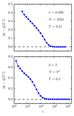
Figure 1: (Color online) Absolute difference between $q_{l}$ and the quantity $q_{l}^{\prime}(U)\equiv(2T/z)U+1$, obtained from the equilibrium relationship of Eq. (8), for the LR model with $N=1024,\sigma=0.896$ (top panel) and the 3D EA model with $L=8$ (lower panel) as a function of Monte Carlo sweeps ($t$) on a log-linear scale. At large times the difference is zero, but the simulation continues well beyond this point to ensure that good statistics are obtained for all samples. Error bars are smaller than the symbols. Both panels have the same horizontal scale.

As an additional check on equilibration for the 1D LR models, Fig. 2 shows several quantities of interest, defined in Sec. IV, as a function of the number of sweeps on a log scale, for the lowest temperature studied and for each value of $\sigma$. The data appear to have saturated.

The 3D EA data set has also been tested for equilibration using the integrated autocorrelation time, as discussed in Ref. Yucesoy et al., 2013a.

IV Measured Quantities

For a single sample ${\mathcal{J}}\equiv\{J_{ij}\}$, the spin overlap distribution $P_{\mathcal{J}}(q)$ is given by

$$P_{\mathcal{J}}(q)=\left\langle\delta\left(\,q-{1\over N}\sum_{i=1}^{N}S_{i}^{(1)}S_{i}^{(2)}\,\right)\right\rangle\,,$$ (11)

where “$(1)$” and “$(2)$” refer to two independent copies of the system with the same interactions, and $\langle\cdots\rangle$ denotes a thermal (i.e., Monte Carlo) average for the single sample. In most previous work, $P_{\mathcal{J}}(q)$ is simply averaged over disorder samples to obtain $P(q)$ defined by

$$P(q)=\left[P_{\mathcal{J}}(q)\right]_{\mathrm{av}}\,.$$ (12)

(a) $\Delta(q_{0}=0.2,\,\kappa=1)$

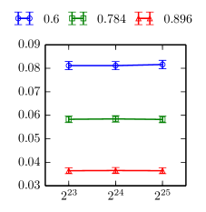
(b) $I^{\text{av}}(q=0.2)$

(c) $I^{\text{med}}(q=0.2)$

Figure 2: (Color online) Plots of several observables obtained from the overlap distribution, defined in Sec. IV, vs the number of Monte Carlo sweeps for the largest size studied, $N=1024$, for the long-range model at the lowest temperature simulated for each value of $\sigma$. (See Table 1.)

In order to gain additional information that might distinguish the RSB and droplet pictures, several investigators have recently introduced other observables related to the statistics of $P_{\mathcal{J}}(q)$. Yucesoy et al.Yucesoy et al. (2012) proposed a measure that is sensitive to peaks in the overlap distributions of individual samples. A sample is counted as “peaked” if $P_{\mathcal{J}}(q)$ exceeds a threshold value $\kappa$ in the domain $\mathinner{\!\left\lvert q\right\rvert}<q_{0}$. The quantity $\Delta(q_{0},\,\kappa)$ is then defined as the fraction of peaked samples. More precisely, for each sample let

$$\Delta_{\mathcal{J}}(q_{0},\,\kappa)=\begin{cases}1,&\mathrm{if}\ P_{\mathcal{J}}^{\mathrm{max}}(q_{0})>\kappa,\\ 0,&\mathrm{otherwise,}\end{cases}$$ (13)

where $P_{\mathcal{J}}^{\mathrm{max}}(q_{0})$ is the maximum value of the distribution in the domain specified by $q_{0}$,

$$P_{\mathcal{J}}^{\mathrm{max}}(q_{0})=\max\{P_{\mathcal{J}}(q)\mathrel{\mathop{\mathchar 58\relax}}\,\mathinner{\!\left\lvert q\right\rvert}<q_{0}\}.$$ (14)

We then define $\Delta(q_{0},\,\kappa)$ to be the sample average,

$$\Delta(q_{0},\,\kappa)=\left[\Delta_{\mathcal{J}}(q_{0},\,\kappa)\right]_{\mathrm{av}}.$$ (15)

The quantity $\Delta(q_{0},\kappa)$ is a nondecreasing function of $q_{0}$ and a nonincreasing function of $\kappa$. This behavior follows simply from the definition of $\Delta(q_{0},\kappa)$. A more important property of $\Delta(q_{0},\,\kappa)$ is that it must go either to zero or one as $N\rightarrow\infty$.com (b) All the scenarios for the low-temperature behavior of spin-glass models predict that $P_{\mathcal{J}}(q)$ consists of $\delta$ functions as $N\rightarrow\infty$. The difference between scenarios lies in the number and position of these $\delta$ functions. The RSB picture predicts that there is a countable infinity of $\delta$ functions that densely fill the line between $-q_{\rm EA}$ and $+q_{\rm EA}$. Thus, for any $q_{0}$ and any $\kappa$, $\Delta(q_{0},\,\kappa)\rightarrow 1$ for models described by RSB. On the other hand, for models described by the droplet scenario or other single pair of states scenarios, $\Delta(q_{0},\,\kappa)\rightarrow 0$ for any $q_{0}<q_{\rm EA}$ and any $\kappa$. Thus, the quantity $\Delta(q_{0},\,\kappa)$ will sharply distinguish the RSB and droplet scenarios if one can study large enough sizes. We shall study the size dependence of $\Delta$ numerically for all our models in Sec. V.1.

As mentioned above, most previous work evaluated the average probability distribution $P(q)$, but recently Middleton,Middleton (2013) and Monthus and Garel,Monthus and Garel (2013) have proposed measures yielding a typical value of the sample distribution $P_{\mathcal{J}}(q)$ in the hopes that these measures would provide a clearer differentiation between the RSB and droplet pictures than the average $P(q)$.

MiddletonMiddleton (2013) studied $I^{\text{med}}(q)$, the median of the cumulative overlap distribution of a single sample $I_{\mathcal{J}}(q)$, where $I_{\mathcal{J}}(q)$ is defined by

$$I_{\mathcal{J}}(q)=\int_{-q}^{q}P_{\mathcal{J}}(q^{\prime})\operatorname{d\!}q^{\prime}.$$ (16)

We also denote the average cumulative distribution over samples by $I^{\text{av}}(q)$, which is given by

$$I^{\text{av}}(q)=\int_{-q}^{q}P(q^{\prime})\operatorname{d\!}q^{\prime}\,.$$ (17)

The median is insensitive to the effect of samples with unusually large values of $I_{\mathcal{J}}(q)$.

For the SK model $P(q)$ tends to a constant as $q\to 0$, and so $I^{\text{av}}(q)\propto q$ for small $q$. We can obtain a rough idea of how $I^{\text{med}}(q)$ varies with $q$ for small $q$ in the SK model from the results of Mézard et al.Mézard et al. (1984) First of all, to obtain a notation which is more compact and is extensively used in other work, we write $x(q)\equiv I^{\text{av}}(q)$. Mézard et al.Mézard et al. (1984) argue that, at small $q$ where $x(q)$ is also small, the probability of a certain integrated value $I_{\mathcal{J}}$ is given by

$$p(I_{\mathcal{J}})\propto x\,I_{\mathcal{J}}^{x-1}\,,$$ (18)

where we recall that $x$ is the average value of $I_{\mathcal{J}}$. From Eq. (18) we estimate the median in terms of the average as

$$I^{\text{med}}(q)\propto e^{-\ln 2/x(q)}=e^{-\ln 2/[2qP(0)]}$$ (19)

for $q\to 0$, where we used that $P(0)$ is nonzero so $x(q)\equiv I^{\text{av}}(q)\simeq 2P(0)\,q$ in this limit [see Eq. (17)]. Hence the median tends to zero exponentially fast as $q\to 0$ whereas the average only goes to zero linearly.

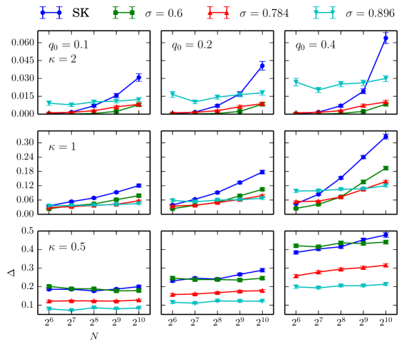
Figure 3: (Color online) $\Delta(q_{0},\,\kappa)$ as a function of system size $N$ for the long-range models and the SK model for all available values of $\sigma$ and various values of the window $q_{0}$ and threshold $\kappa$. In all cases the temperature is $0.4T_{c}$. All panels have the same horizontal scale, and all panels in a row have the same vertical scale.

In the droplet picture, $P(0)$ is expected to vanish with $L$ asFisher and Huse (1986) $L^{-\theta}$, so $I^{\text{av}}(q)\propto L^{-\theta}\,q$ for small $q$. The median value $I^{\text{med}}(q)$ will presumably also vanish for small $q$ as $L\to\infty$, but we are not aware of any precise predictions for this. We shall study the median cumulative distribution numerically in Sec. V.2.

Another measure related to the overlap distribution of individual samples has been proposed by Monthus and Garel.Monthus and Garel (2013) They suggest calculating a “typical” overlap distribution defined by the exponential of the average of the log as

$$P^{\text{typ}}(q)=\exp\left[\ln P_{\mathcal{J}}(q)\right]_{\mathrm{av}}\,.$$ (20)

We shall study this quantity numerically in Sec. V.3.

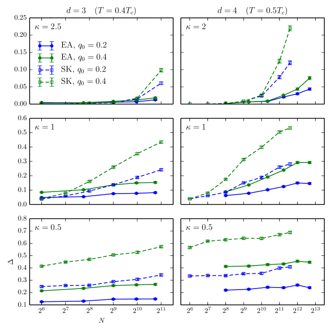
Figure 4: (Color online) $\Delta(q_{0},\,\kappa)$ as a function of system size $N$ for the short-range models and the SK model for several values of the window $q_{0}$ and threshold value $\kappa$. The points connected by solid lines are for the EA models, while those connected by dashed lines are for the SK model. The temperatures are $0.4T_{c}$ for the 3D data and $0.5T_{c}$ for the 4D data. All panels in a column have the same horizontal scale and all panels in a row have the same vertical scale.

V Results

V.1 Fraction of peaked samples, $\Delta(q_{0},\kappa)$

Plots of $\Delta(q_{0},\kappa)$ for the 1D long-range models for various values of $q_{0}$ and $\kappa$ at $T\approx 0.4T_{c}$ are given in Fig. 3, while the corresponding plots for the 3D and 4D models are shown in Fig. 4. A comparison with the SK model is made in both cases. The error bars for all plots in this section are one standard deviation statistical errors due to the finite number of samples. There are also errors in the data for each sample due to the finite length of the data collection. For the EA and SK models, we estimated these errors by measuring $\Delta^{+}(q_{0},\kappa)$ and $\Delta^{-}(q_{0},\kappa)$, defined as in Eqs. (13) – (15) but from the $q>0$ and $q<0$ components of $P_{\mathcal{J}}(q)$, respectively. These are expected to be reasonably independent and their differences provide an estimate of the error due to finite run lengths. For all sizes, the average absolute difference between these quantities, $[|\Delta^{+}(q_{0},\kappa)-\Delta(q_{0},\kappa)|+|\Delta^{-}(q_{0},\kappa)-\Delta(q_{0},\kappa)|]/2$, is less than the statistical error. While a similar analysis was not done for the 1D LR models, measurements of $\Delta$ versus the number of sweeps shown in Fig. 2 suggest that the data have saturated within statistical error.

One can draw several qualitative conclusions from these plots. It is apparent that $\Delta(q_{0},\kappa)$ is an increasing function of $N$ for small $N$. As the system size increases, we expect $\Delta(q_{0},\kappa)$ to increase because all the features of $P_{\mathcal{J}}(q)$ sharpen. For the SK model, which is indisputably described by the RSB picture, the number of features and their height should both increase and $\Delta(q_{0},\kappa)$ should be a strongly increasing function of $N$. Indeed, this behavior is seen except for $\kappa=0.5$, which is a sufficiently small value that $\Delta(q_{0},\kappa)$ is effectively measuring whether or not there is a feature in the relevant range, and this quantity increases relatively slowly for the SK model.

However, as $\sigma$ increases for the 1D models, the curves become increasingly flat and the difference between $\sigma=0.896$ and the SK model is striking; the former is nearly flat while the latter increases sharply (see Fig. 3). The same qualitative distinction holds between the 3D EA model and the SK model (see Fig. 4). The similarity between the behavior of the 1D model for $\sigma=0.896$ and the 3D EA model is expected since the two models are believed to have the same qualitative behavior. The distinction between the SK model and the 1D model with $\sigma=0.784$ and the 4D EA model is less striking but qualitatively the same.

It is interesting to compare results for the SK model with the 1D model with $\sigma=0.6$, which is in the mean-field regime. For $\kappa=0.5$ the results for the two models are very similar, and do not increase much with $N$, indicating that $\kappa=0.5$ is too small to give useful information for this range of sizes, as discussed above. For $\kappa=1$, the SK data increase the most rapidly with $N$, and the $\sigma=0.6$ data increase less quickly, but still faster than the other values of $\sigma$. For $\kappa=2$, the SK data increase quickly, while for the value of $\sigma$ furthest from the SK limit, $0.896$, the data are moderately large but roughly size independent over the range of sizes simulated. Curiously, for intermediate values of $\sigma$ ($0.6$ and $0.784$) the data are very small but show an increase for the larger sizes. This increase is particularly sharp for $\sigma=0.6$. It seems that there is an initial value of $\Delta$ for small $N$ and a growth as $N$ increases. We do not have a good understanding of the initial value, e.g., why it is so small for $\kappa=2$ and $\sigma=0.6$, and $0.784$. The more important aspect of the data is the increase observed, at least for most parameter values, at large sizes. Given the rapid increase in the data for $\sigma=0.6,\kappa=2$ for the largest size, we anticipate that for still larger sizes, its value for $\Delta$ for $\kappa=2$ would be closer to that of the SK model than that of the intermediate $\sigma$ values.

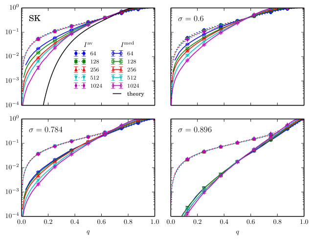
Figure 5: (Color online) Mean and median over samples of the integrated distribution $I_{\mathcal{J}}(q)$ for the long-range models and the SK model. In all cases the temperature is close to $0.4T_{c}$. For both the SK model and the 1D models, the median shows a relatively strong size dependence compared with the mean, this difference being the least pronounced for $\sigma=0.896$. The “theory” curve for the SK data [Eq. (19)] is expected to be valid for small $q$ only. The theory expression can be multiplied by an (unknown) constant which has been set to unity. All panels have the same horizontal and vertical scales.

There are two possible interpretations of the trends discussed above. If one believes that the RSB picture holds for all of the models studied here, then one can point to the fact that all the $\Delta$ curves are nondecreasing and assert that they will all approach unity as $N\rightarrow\infty$, just extremely slowly for the 3D EA model and the 1D $\sigma=0.896$ model. An argument supporting this idea is made in Ref. Billoire et al., 2012 and rebutted in Ref. Yucesoy et al., 2013b. If on the other hand, one believes the droplet scenario or the chaotic pair scenario holds for finite-dimensional spin glasses, then the flattening of the curves for these models is a prelude to an eventual decrease to zero. Unfortunately, the sizes currently accessible to Monte Carlo simulation do not permit one to sharply distinguish between these competing hypotheses. Using an exact algorithm for the two-dimensional (2D) Ising spin glass with bimodal disorder, MiddletonMiddleton (2013) shows that the crossover to decreasing behavior for $\Delta(q_{0},\kappa)$ in 2D does occur at large length scales. He also shows within a simplified droplet model, that the large length scales are needed to see the predictions of the droplet scenario manifest in the 3D EA model. Overall, we see that we need larger sizes to unambiguously determine from $\Delta(q_{0},\kappa)$ whether the droplet or RSB picture applies to 3D-like models.

V.2 Median $I^{\text{med}}(q)$ and mean $I^{\text{av}}(q)$ cumulative overlap distribution

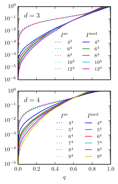
Figure 6: (Color online) Log-linear plot of $I^{\text{med}}(q)$ and $I^{\text{av}}(q)$ vs $q$ plot for the 3D EA model at $T\simeq 0.42$ (upper panel) and for the 4D EA model at $T\simeq 0.90$ (lower panel). Both panels have the same horizontal scale.

In this section, we compare the mean $I^{\text{av}}(q)$ and the median $I^{\text{med}}(q)$ of the cumulative overlap distribution. Figure 5 shows results for $I^{\text{av}}(q)$ and $I^{\text{med}}(q)$ for the SK model and several long-range models for a temperature close to $0.4T_{c}$. Figure 6 shows the same quantities for the 3D EA and 4D EA models.

As noted in earlier work, the results for the average show very little size dependence for all models. This is a prediction of the RSB picture which certainly applies to the SK model. By contrast, in the droplet picture $I^{\text{av}}(q)$ is predicted to vanish asFisher and Huse (1986) $L^{-\theta}$. The observed independence of $I^{\text{av}}(q)$ with respect to $L$ is one of the strongest arguments in favor of the RSB picture for finite-dimensional Ising spin-glass models. However, it has been argued, e.g., Refs. Moore et al., 1998; Middleton, 2013, that there are strong finite-size corrections and that the asymptotic behavior predicted by the droplet model for $I^{\text{av}}(q)$ would only be seen for sizes larger than those accessible in simulations. This is why the median has been proposedMiddleton (2013) as an alternative to the mean.

The data for the median of the SK model in Fig. 5 show a rapid decrease at small $q$, which is very strongly size dependent. As discussed in Sec. IV above, the rapid decrease is expected in the RSB picture since it predicts that $I^{\text{med}}(q)$ is exponentially small in $1/q$ [see Eq. (19)]. The theoretical result is shown as a solid line in the SK panel. It is plausible that the data will approach the theory in the large $N$ limit, but there are strong finite-size effects at small $q$ for the sizes that can be simulated, so the data for the largest sizes are still far from the theoretical prediction. This already indicates that the median is not a very useful measure to distinguish the RSB picture from the droplet picture.

The median data for the long-range 1D model with $\sigma=0.6$, which is in the mean-field region, shows similar trends to that for the SK model. On the other hand, for the long-range model furthest from mean-field theory, $\sigma=0.896$, the data also decrease rapidly at small $q$ but are less dependent on size. The data for the 3D and 4D EA models in Fig. 6 also show a rapid decrease at small $q$, which is quite strongly size dependent.

We have seen that even for the SK model it would be very difficult to extrapolate the numerical data to an infinite system size. For the long-range models, the most likely candidate for droplet theory behavior, according to which the median (such as the average) vanishes in the thermodynamic limit, is $\sigma=0.896$. However, for this model, the data are not zero for small $q$ and there is rather little size dependence, implying that, if the droplet picture does hold, it will only be seen for much larger sizes than can be simulated. This is the same situation as for the mean (if the droplet picture is correct). Consequently, it does not seem to us that the median of the cumulative order parameter distribution is a particularly useful quantity to distinguish the droplet and RSB pictures.

V.3 Typical overlap distribution, $P^{\text{typ}}(q)$

Estimating $P^{\text{typ}}(q)$—defined in Eq. (20) as the exponential of the average of the logarithm—from Monte Carlo simulations is problematic because the finite number of observations means that the result can be precisely zero if the average is comparable to, or smaller than, $\epsilon$, the inverse of the number of measurements. Such results make the typical value undefined according to Eq. (20). One can regularize this problem by replacing zero values of $P_{\mathcal{J}}(q)$ with the small value $\epsilon/k$ for a reasonable range of $k$, in the hope that the result would not be too sensitive to the choice of $k$. Unfortunately, there is a strong dependence on $k$, as seen in Fig. 7, where $P^{\text{typ}}(q)$ is plotted for several values of $k$ for the SK model for $N=2048$. The dependence on $k$ indicates that $P^{\text{typ}}(q)$ cannot be reliably measured in Monte Carlo simulations with feasible run lengths.

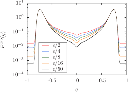
Figure 7: (Color online) Log-linear $P^{\rm typ}(q)$ plot for the SK model for $N=2048$ showing the strong dependence on the zero-replacement value $\epsilon/k$. See the main text for details.

VI Summary and Conclusions

We have studied the overlap distribution for several Ising spin-glass models using recently proposed observables. We consider 1D long-range models, 3D and 4D short-range (Edwards-Anderson) models, and the infinite-range (Sherrington-Kirkpatrick) model. The three observables are all obtained from the single-sample overlap distribution $P_{\mathcal{J}}(q)$. They are the fraction of peaked samples $\Delta(q_{0},\kappa)$, the integrated median $I^{\text{med}}(q)$, and the typical value $P^{\text{typ}}(q)$. These observables were proposed to help distinguish between the replica symmetry breaking picture and two-state pictures such as the droplet model. While none of these statistics unambiguously differentiates between these competing pictures, it appears that $\Delta$ does the best job. In particular, there is a qualitative distinction between the behavior for the 3D EA model and the long-range 1D model with $\sigma=0.896$ that is expected to mimic it, on the one hand, and the mean-field SK model and the 1D model with $\sigma=0.6$ that is expected to be in the mean-field regime, on the other hand. For a reasonable range of $q_{0}$ and $\kappa$, the two 3D-like models do not show an increase in $\Delta$ for the largest sizes while the mean-field models are sharply increasing for the largest sizes. The increase in $\Delta$ for the mean-field model is exactly what we expect from the RSB picture. The results for the 3D-like models are ambiguous because eventually $\Delta$ must go either to zero or one. It is possible that for much larger sizes $\Delta$ will begin to increase, indicating RSB behavior, but simulating such large system sizes at very low temperatures is unfeasible at present.

The other proposed measures do not appear to be useful in numerical simulations for distinguishing scenarios. The typical value of the overlap $P^{\text{typ}}(q)$ cannot be measured in feasible Monte Carlo simulations while the median value of the cumulative overlap $I^{\text{med}}(q)$ is very small at small $q$ even for the SK model and has a very strong size dependence. For the droplet model $I^{\text{med}}(q)$ is presumably zero at small $q$ for $N\to\infty$. However, the strong size dependence of the results in this region of small $q$ makes it impossible to tell numerically, if the data are going to zero or just to a very small value, even for the SK model. Curiously, there is less size dependence for the 3D model and the equivalent 1D with $\sigma=0.896$ than for the SK model.

Recently, we became aware of a related paper by Billoire et al.Billoire et al. (2014). Reference Billoire et al., 2014 argues that the data for $I^{\text{med}}(q)$ for the SK model “converge nicely to some limiting curve when $N$ increases” and that “trading the average for the median does make the analysis more clear cut.” In contrast, we find a strong finite-size dependence for $I^{\text{med}}(q)$ for the SK model in the important small-$q$ region (clearly visible in a logarithmic scale) and largely because of this we do not find that the median is particularly helpful in distinguishing between the droplet and RSB pictures.