Jamming in Hierarchical Networks

Abstract

We study the Biroli-Mezard model for lattice glasses on a number of hierarchical networks. These networks combine certain lattice-like features with a recursive structure that makes them suitable for exact renormalization group studies and provide an alternative to the mean-field approach. In our numerical simulations here, we first explore their equilibrium properties with the Wang-Landau algorithm. Then, we investigate their dynamical behavior using a grand-canonical annealing algorithm. We find that the dynamics readily falls out of equilibrium and jams in many of our networks with certain constraints on the neighborhood occupation imposed by the Biroli-Mezard model, even in cases where exact results indicate that no ideal glass transition exists. But while we find that time-scales for the jams diverge, our simulations can not ascertain such a divergence for a packing fraction distinctly above random close packing. In cases where we allow hopping in our dynamical simulations, the jams on these networks generally disappear.

I Introduction

The jamming transition, as discussed by Liu and Nagel in 1998 Liu and Nagel (1998), for example, has been the focus of intense study Biroli (2007); Liu and Nagel (2010). A granular disordered system for increasing density can reach a jammed state at which a finite yield stress develops, or at least extremely long relaxation times ensue, similar to the emerging sluggish behavior observed when the viscosity of a cooled glassy liquid seemingly diverges. Thus, a jamming transition may be induced in various ways, such as by increasing density, decreasing temperature, or/and reducing shear stress Liu and Nagel (2010). Below the jamming transition, the system stays in long-lived meta-stable states, and its progression to its corresponding equilibrium state entails an extremely slow, non-Debye relaxation Hill and Dissado (1985); Ciamarra et al. (2010); Van Hecke (2010). Jamming transitions have been observed in various types of systems, such as granular media Majmudar et al. (2007), molecular glasses Parisi and Zamponi (2010); Angelani and Foffi (2007), colloids Trappe et al. (2001), emulsions Zhang and Makse (2005), foams Berthier et al. (2011); Da Cruz et al. (2002), etc Liu and Nagel (2010); Van Hecke (2010). These systems can behave like stiff solids at a high density with low temperature and small perturbations. In these transitional processes, the systems can self-organize their own structure to avoid large fluctuations Berthier et al. (2011) and to reach a quasi-stable jammed state, characterized by an extremely slow evolution to the unjammed equilibrium state. The properties of those quasi-stable non-equilibrium states as well as their corresponding equilibrium state is the main focus of this paper.

The properties of the jamming transition have been studied extensively Biroli (2007); Majmudar et al. (2007); Liu and Nagel (2010), but we still lack an essential understanding of the physics underlying the jammed state. Theoretical progress has been much slower than the accumulation of experimental discoveries. One of the reasons is the scarcity of theoretical microscopic models to capture the complex jamming process Krzakala et al. (2008); Jacquin et al. (2011). In recent years, a lattice glass model proposed by Biroli and Mezard (BM) Biroli and Mezard (2002) has been shown as a simple but adequate means to study the jamming process. It is simple because the model follows specific dynamical rules which are elementary to implement in both simulations and analytical work. In distinction to kinetically constrained models such as that due to Kob and Andersen Kob and Andersen (1993), in which particles are blocked from leaving a position unless certain neighborhood conditions are satisfied, BM embeds geometric frustration merely by preventing the neighborhood of any particles to consist of more than $l$ other particles. Beyond that, it proceeds purely thermodynamically. The phase diagram can be reduced to just one (or both) of two control parameters, chemical potential and temperature. Either is sufficient to reproduce a jamming transition which is similar to that observed in off-lattice systems Biroli and Mezard (2002). Using this model in a mean-field network (i.e., a regular random graph), Krzakala et al. find jammed states in Monte Carlo simulations and a genuine thermodynamical phase transition (ideal glass transition) in its mean-field analytical solutions Krzakala et al. (2008). In other words, the jammed state coincides with an underlying equilibrium state that possesses a phase transition to a glassy state. That raises the prospect that this glass transition might be the reason for the onset of jamming. The evidence for such a connection thus far is based on mean-field models Biroli and Mezard (2002); Krzakala et al. (2008); Rivoire et al. (2003), as such a transition is hard to ascertain for finite-dimensional lattice glasses. Yet, it remains unclear whether mean-field solutions in disordered systems can provide an adequate conception for real-world behavior.

In this paper, we propose to use the lattice glass model BM on hierarchical networks Boettcher et al. (2008), which are networks with a fixed, lattice-like geometry. They combine a finite-dimensional lattice backbone with a hierarchy of small-world links that in themselves impose a high degree of geometric frustration despite of their regular pattern. In fact, the recursive nature of the pattern can ultimately provide analytical solution via the renormalization group (RG), positioning these networks as sufficiently simple to solve as well as sufficiently lattice-like to become an alternative to mean-field solutions Boettcher and Hartmann (2011). Unlike mean-field models, our network is dominated by many small loops that are also the hallmark of lattice systems. Our goal is to find (1) whether the lattice glass model leads to jamming state in hierarchical networks, (2) whether there is an ideal glass transition underlying the jamming transition, and (3) whether the local dynamics affect the jamming process. To our knowledge, these questions have not been studied in any small-world systems. Our results can contribute new insights to understand jamming.

We find that BM in these networks can jam, even when there is certifiably no equilibrium transition; the geometric frustration that derives from the incommensurability among the small-world links is sufficient in many cases to affect jamming. In fact, jamming is most pronounced for fully exclusive neighborhoods ($l=0$). It disappears for more disordered neighborhoods ($l=1$), at least for our non-regular networks, where the allowance of $l=1$ neighbor to be occupied seems to provide the “lubrication” that averts jams. However, the packing fractions at which time-scales diverge is virtually indistinguishable from random close packing within the accuracy of our simulations.

Mean-field calculations of BM in Ref. Rivoire et al. (2003) predict a kinetic transition for dynamic rules based on nearest-neighbor hopping. In our simulations, we find that such hopping, in addition to the particle exchange with a bath, can affect a dramatic change in the dynamic behavior and eliminated jamming in all cases we consider.

This paper is organized as follows. In Sec. II, we describe the model, the networks, and out numerical simulations. In Sec. III we discuss the results of our simulations for each network. In Sec. IV we conclude with a few summary remarks and an outlook for future work.

II Model & Methods

In this section, we describe the model and the networks on which we will study its behavior. To benchmark the equilibrium properties of the model on those networks, we implement a multi-canonical algorithm due to Wang and Landau Wang and Landau (2001a, b). We further need a grand-canonical annealing algorithm to study the dynamics of the lattice glass model on those networks.

II.1 Lattice glass model

The lattice glass model as defined by Biroli and Mezard (BM) Biroli and Mezard (2002) considers a system of particles on a lattice of $N$ sites. Each site can carry either $x_{i}=0$ or $x_{i}=1$ particle, and the occupation is restricted by a hard, local “density constraint”: any occupied site ($x_{i}=1$) can have at most $l$ occupied neighbors, where $l$ could range locally from 0 to the total number of its neighbor-sites. In this model, the jamming is defined thermodynamically by rejecting the configurations violating the density constraint. Here, we focus on global density constraints of $l=0$ (completely excluded neighborhood occupation) and $l=1$ as the most generic cases. The system can be described by the grand canonical partition function

$$Z(\mu)=\sum_{{\bf allowed}\,\{x_{i}\}}\exp\left[\mu\sum_{i=1}^{N}x_{i}\right],$$ (1)

where the sum is over all the allowed configurations $\{x_{i}\}$. Here, $\mu$ is the reduced chemical potential, where we have chosen units such that the temperature is $k_{B}T=1/\beta=1$, and $\sum_{i=1}^{N}x_{i}$ is the total number of particles in a specific configuration.

From the grand canonical partition function in Eq. (1), we can obtain the thermodynamic observables we intend to measure, such as the Landau free energy density $w(\mu)$, the packing fraction $\rho(\mu)$, and the entropy density $s\left[\rho(\mu)\right]$, as defined in the following equations:

$$w(\mu) = -\frac{1}{N}\ln Z,$$ (2)

$$\rho(\mu) = \frac{1}{N}\left<\sum_{i=1}^{N}x_{i}\right>_{\mu}=\frac{1}{N}\frac{\partial\ln Z}{\partial\mu},$$

$$s(\mu) = \frac{1}{N}\left(1-\mu\frac{\partial}{\partial\mu}\right)\ln Z.$$

II.2 Hierarchical networks

In our investigations, we use the Hanoi networks  Boettcher et al. (2008). These are small-world networks with a hierarchical, recursive structure that avoid the usual randomness involved in defining an ensemble of networks. Thus, no additional averages of such an ensemble are required to obtain scaling properties in thermodynamical limit from a finite system size, which reduces the computational effort. Hanoi networks combine a real-world geometry with a hierarchy of small-world links, as an instructive intermediary between mean-field and finite-dimensional lattice systems, on which potentially exact results can be found using the renormalization group Boettcher and Hartmann (2011).

We use three Hanoi networks: HN3 is a network with a regular degree of 3, while HN5 is a similar network that possesses many extra links such that vertices have an exponential arrangement of degrees with an average degree of 5. HNNP is a similar Hanoi network of average degree of 4, but which is non-planar. Each of them can be built on a simple backbone of a 1D lattice. The 1D backbone has $N=2^{k}+1$ ($k=1,2,3,\cdots$) sites where each site is numbered from $0$ to $N$. Any site $n$, $0\leq n\leq N$, can be defined by two unique integers $i$ and $j$,

$$n(i,j)=2^{i-1}(2j+1),$$ (3)

where $i$, $1\leq i\leq k$, denotes the level in the hierarchy and $j$, $0\leq j<2^{k-i}$, labels consecutive sites within each hierarchy $i$. Site $n=0$ is defined in the highest level $k$ or, equivalently, is identified with site $n=N$ for periodic boundary conditions. With this setup, we have a 1D backbone of degree 2 for each site and a well-defined hierarchy on which we can build long-range links recursively in three different ways: HN3 Boettcher et al. (2008) is constructed by connecting the neighbor sites $n(i,0)\longleftrightarrow n(i,1)$, $n(i,2)\longleftrightarrow n(i,3)$, $n(i,4)\longleftrightarrow n(i,5)$, and so on and so forth. For example, in level $i=1$, site $n(1,0)=1$ is connected to $n(1,1)=3$; site $n(1,2)=5$ is connected to $n(1,3)=7$; and so on. A initial section of a HN3 network is given in Fig. 1. As a result, HN3 is a planar network of regular degree 3.

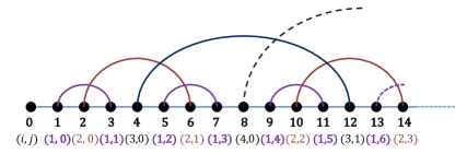
Figure 1: An example of the first 14 sites of HN3 on a semi-infinite line.

HN5 Boettcher et al. (2009), as shown in Fig. 2, is an extension based on HN3, where each site in level $i$ ($i\geq 2$, i.e., all even sites) is further connected to sites that are $2^{i-1}$ sites away in both directions. For example, for the level $i=2$ sites (sites $2,6,10,\cdots$), site 2 is connected to both site 0 and site 4; site 6 is connected to sites 4 and 8; etc. The resulting network remains planar but has a hierarchy-dependent degree, i.e., 1/2 sites have degree 3, 1/4 have degree 5, 1/8 have degree 7, etc. In the limit of $N\to\infty$, this network has average degree 5.

HNNP Boettcher et al. (2009), also shown in Fig. 2, is constructed from the same 1D backbone as HN3 and HN5. However, for site $n$ in level $i$ with even $j$, it is connected forwards to site $(n+3\times 2^{i-1})$; while site $n$ in level $i$ with odd $j$ is connected backwards to site $(n-3\times 2^{i-1})$. Level 1 and level 2 sites have degree 3, and level $3,4,5,\cdots$ sites have degree $5,7,9,\cdots$. The HNNP has an average degree of 4 and is non-planar.

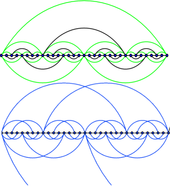
Figure 2: Depiction of HN5 (top) and HNNP (bottom), first introduced in Ref.  Boettcher et al. (2009). Green-shaded lines in HN5 represent its difference to HN3, which is at its core (dark lines). While HN3 and HN5 are planar, HNNP is non-planar.

II.3 Wang-Landau Sampling

Wang-Landau sampling Wang and Landau (2001a) is a multi-canonical method to numerically determine the entire density of states $g_{n}$ within a single simulation. This method is based on the fact that a random walk in the configuration space with a probability proportional to the inverse of the density of states with occupation $n$, $0\leq n\leq N$, enforces a flat histogram in $g_{n}$ over all $n$. Based on this fact, Wang-Landau sampling keeps modifying the estimated density of states in the random walks over all possible configurations and can make the density of states converge to the true value. The update procedure is:

1. Initially, set all unknown density of states $\{g_{n}=1\}$ and the histogram $\{H_{n}=0\}$ for all occupations $n$, initiate the modification factor $f=e^{1}\approx 2.71828\dots$ ;

2. Randomly pick a site $i$; if it is empty (occupied), add (remove) a particle with a probability of $\min\left[1,\frac{g_{n}}{g_{n+1}}\right]$ ($\min\left[1,\frac{g_{n}}{g_{n-1}}\right]$) while obeying the rule of the hard local density constraint on having at most $l$ occupied nearest neighbors of site $i$;

3. Randomly pick one occupied site and one empty site; transfer a particle from the occupied site to the empty, if the density constraint is not violated;

4. Update the $H_{n}$ and $g_{n}$ of the current state, i.e., set $\{H_{n}=H_{n}+1\}$ and $\{g_{n}=g_{n}\times f\}$;

5. Repeat steps 2 to 4 until the sampling reaches a nearly flat histogram for the $H_{n}$, then update the modification factor $f=\sqrt{f}$ and reset $\{H_{n}=0\}$;

6. Stop if $f\leq 1+10^{-8}$.

Our procedure mostly follows the standard procedure of Wang-Landau sampling Wang and Landau (2001a), except for step 3. Its purpose is to facilitate the random walk to explore phase space more broadly and to expedite convergence.

Wang-Landau sampling has been proved as an effective method to find the density of states Wang and Landau (2001a); Lee et al. (2006); Cunha-Netto and Dickman (2011). In our study, it can find convergence for system size of up to $N\sim 10^{3}$ within a reasonably computational cost. From the density of states, we can calculate the equilibrium thermodynamical properties for the corresponding system sizes.

II.4 Grand-Canonical Annealing

In parallel to the equilibrium properties provided by Wang-Landau sampling, we also implement a form of simulated annealing Kirkpatrick et al. (1983) to explore the dynamics of the model and the possibility of jamming, in a process that is similar to an experiment. Simulated annealing used in this study follows the standard procedure  Černỳ (1985). The corresponding experiment is exchanging particles between the network and a reservoir of particles with (dimensionless) chemical potential $\mu$. In our study, the annealing speed is not controlled by decreasing temperature (which we set to $\beta=1$) but by increasing the chemical potential. The annealing algorithm is:

1. Initially, start with chemical potential $\mu_{0}=0$ ;

2. Randomly pick a site $n$; if it is empty (occupied), add (remove) a particle with a probability of $\min\left[1,\exp(\mu)\right]$ ($\min\left[1,\exp(-\mu)\right]$) while obeying the rule of the hard local density constraint on having at most $l$ occupied nearest neighbors of $n$;

3. If hopping is allowed, randomly pick one site; only if it is occupied, randomly pick one of its empty neighbor(s) and displace the particle if the density constraint remains satisfied;

4. Increase $\mu$ by $d\mu$ every 1 Monte Carlo sweep ($N$ random updates), where $d\mu/dt$ (in time-units of $dt=1$) is the annealing schedule and $d\mu\ll 1$;

5. Repeat steps 2 to 4 until $\mu$ reaches a certain (large) chemical potential.

Following the procedure above, the simulated annealing can reveal whether or not a jamming transition occurs in the process. Besides that, we can test the effect of local dynamics Biroli and Mézard (2002); Krzakala et al. (2008) by adding a local hopping random walk (step 3), i.e., a particle can transfer any of its empty neighboring sites as long as the constraint remains satisfied. The results are shown and explained in the following section.

III Results

To assess the properties of jamming, we first have to benchmark our systems with the corresponding equilibrium behaviors. After that, we discuss the dynamic simulations with the annealing algorithm in reference to these equilibrium benchmarks.

III.1 Equilibrium Properties

Wang-Landau sampling, as described in Sec. II.3, is ideally suited for our purpose, since it provides access directly to the density of states $g_{n}$ as a function of occupation number $n$, which yields the partition function as

$$Z(\mu)=\sum_{n=0}^{n_{max}}g_{n}e^{n\mu}.$$ (4)

All thermodynamic quantities in the equilibrium can be obtained numerically by summation of the formal derivates of $Z(\mu)$, such as those in Eqs. (2), over all permissible occupation numbers $0\leq n\leq n_{max}<N$. (For all $n_{max}<n\leq N$ it is $g_{n}=0$.)

In Fig. 3, we plot the density of states as a function of the packing fraction, both obtained with Wang-Landau. It becomes apparent that each model has a simple rational value for its optimal ($\mu\to\infty$) “random” close packing fraction $\rho_{CP}=n_{max}/N$. This corresponds to a random packing in the sense that it has a nontrivial entropy density due to geometric disorder (imposed by the lack of translational invariance in the lattice), except for HNNP at $l=0$, which has a unique “crystalline” packing of every odd site being occupied. While these values for $\rho_{CP}$ have been previously obtained with RG for $l=0$ Boettcher and Hartmann (2011), the simulations predict also strikingly simple but nontrivial values for $l=1$, where exact RG is likely not possible. These values are listed in Table 1.

Table 1: Closest packing fractions $\rho_{CP}$ found by Wang-Landau sampling. The values for $l=0$ have been previously obtained with exact RG, the one for HNNP being unique, with every second, odd site occupied. For $l=1$, we also predict exact fractions with nontrivial entropy densities, see Fig. 3.

Network	$l=0$	$l=1$
HN3	3/8 Boettcher and Hartmann (2011)	9/16
HN5	1/3 Boettcher and Hartmann (2011)	1/2
HNNP	1/2	1/2

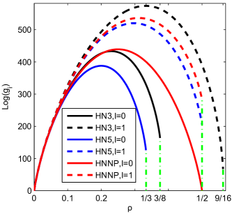
Figure 3: Density of states from Wang-Landau sampling at $N=1024$. The green dash-dot vertical line are showing the closest packing fractions (as shown in Table 1) for each system. Note that only for HNNP at $l=0$ there is a unique, crystalline ground state.

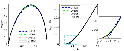
Figure 4: Convergence to the thermodynamic limit for finite system sizes for the example of HN3 with $l=1$ using Wang-Landau sampling. The figures are for the density of states (left) and the packing fraction (right). The equilibrium packing fraction $\rho(\mu)$ as a function of chemical potential $\mu$ is calculated from the density of states according to Eq. (2); it approaches the closest packing fraction $\rho_{CP}$ for $1/\mu\to 0$. The convergence for other systems is similar or better.

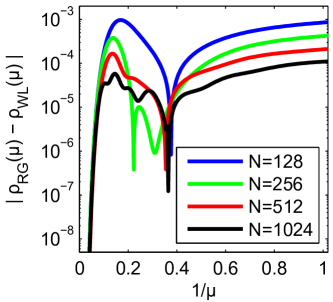
Figure 5: Plot of the error in the finite-size packing fraction in Wang-Landau sampling, $\left|\rho_{WL}-\rho_{RG}\right|$, as a function of $1/\mu$ near close packing ($\mu\to\infty$) in HN3 at $l=0$. Here, RG result $\rho_{RG}(\mu)$ from Ref.  Boettcher and Hartmann (2011) at system size $N=2^{500}$ is taken as the exact, thermodynamic packing fraction. Relative to $\rho_{RG}(\mu)$, the finite-size packing fraction, $\rho_{WL}(\mu)$, at $N=2^{k}$ with $k=8,9,10$ already exhibit quite small and rapidly diminishing corrections.

Wang-Landau sampling converges within a reasonable time for system sizes smaller than $N\approx 2000$ but fails to converge for larger system size. There may be two reasons for the lack of convergence: (1) the density of states is not symmetric as a function of packing fraction, and this asymmetry requires Wang-Landau to sample the whole configuration space, which increases the computational cost dramatically especially for large system sizes; (2) the lower the density of states of the closest packed state, the harder it is for Monte Carlo sampling to find its closest packing state because of the hard-density constraint. Although Wang-Landau sampling fails for large system sizes, the results of system size $N=1024$ can still offer an insight to the equilibrium state because the density of states and the packing fraction exhibit only small finite-size corrections for increasing $N$. For example, the convergence of HN3 with $l=0$ is shown in Fig.4. Other networks with $l=0,1$ have similar or even better convergence.

We can further demonstrate the quality of the Wang-Landau simulations, and appraise their residual finite-size effects, by comparison with exact results obtained with the renormalization group (RG) for $l=0$ on HN3 Boettcher and Hartmann (2011). In Fig. 5, we compare the results for the packing fraction $\rho(\mu)$ as a function of the chemical potential for Wang-Landau sampling on networks with $N=2^{k}$ sites, $k=8\sim 10$, with those from the exact RG after 500 iterations, corresponding to a system of $N=2^{500}$ sites. Despite the much smaller sizes of the Wang-Landau simulation, its results are barely distinguishable from the exact result, affirming the Wang-Landau sampling results as good references for our dynamic simulations, with negligible finite-size effects.

III.2 Dynamic Properties

The dynamic simulations of the BM on our networks uses the grand canonical partition function controlled by a chemical potential $\mu$ that mimics the experimental situation in a complex fluid or colloid, where particles are pumped into the larger system (the reservoir) and can enter the field-of-view through open boundaries inside a smaller window. For example, this could correspond to a $2d$ slice of a $3d$ colloidal bath used in colloidal tracking experiments  Hunter and Weeks (2012). Since our particles are not energetically coupled and merely obey hard excluded volume constraints, temperature is irrelevant and we can set $\beta=1$, making the chemical potential dimensionless, $\beta\mu\to\mu$. As we increase $\mu$, the system is more likely to accept more particles and increase the packing fraction $\rho(\mu)$. When $\mu$ is small (or negative), the reservoir and the network readily reach an equilibrium state with a certain packing fraction. However, when $\mu$ is large, the equilibrium state defined by the partition function has a packing fraction close to the close packing $\rho_{CP}$. Because of the density constraint and the disorder imposed by the hierarchical network geometry, the system enters into a jam at a density far from equilibrium packing. As in experiments, this jammed state remains for an extremely long time, even when $\mu$ is further increased. The ultimate packing fraction $\rho^{*}$ that the systems gets stuck at, in fact, is ever further from random close packing, the faster the quench in $\mu$ is executed, where $\frac{d\mu}{dt}$ is the quench rate. In this, our results closely resemble those reported in Ref. Krzakala et al. (2008).

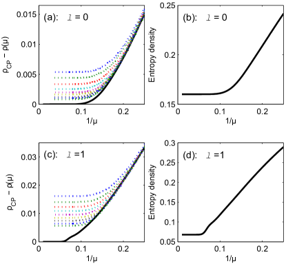
Figure 6: Reduced packing fraction and entropy density for HN3 from Wang-Landau sampling and Simulated Annealing. (a)&(b) are for $l=0$, and (c) &(d) are for $l=1$. The black solid lines represent the equilibrium properties from Wang-Landau sampling with $N=1024$. The dotted lines are from simulated annealing with $N=32,768$, run at different annealing schedules with $d\mu=0.001/2^{j}$ for $j=0,\ldots,8$, from top to bottom. Wang-Landau sampling provides the entropy density via Eq. (2), as shown in (b) and (d), which is difficult to obtain from other Monte Carlo methods. For both, $l=0$ and 1, we find a non-zero entropy density for random close packing at $\mu\rightarrow\infty$.

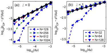
Figure 7: Scaling of the dynamically reached packing fraction $\rho^{*}(d\mu)$ as a function of the annealing rate $d\mu$ for different system sizes $N$ of HN3. (a) For $l=0$, the dashed lines are for systems sizes $N=2^{k}$ with $k=7,\ldots,$10, 12, 14 and 15, from bottom to top. All data sets (except for the smallest sizes, $N=128,\ldots,1024$) collapse onto the top line with a slope of $0.34\pm 0.01$, which is obtained from a fit using the data of the largest system size $N=32,768$. (b) For $l=1$, the data sets converge even faster towards power-law scaling. The dashed lines are for system sizes of $N=2^{k}$ with $k=5,\ldots,8$, 10, 12, 14 and 15, from bottom to top. All but the first 3 sets collapse onto a line of slope $0.19\pm 0.01,$ which is obtained from a fit for $N=32,768$. Error bars are about of the size of each data point or smaller, indicating a relative error of less than $3\%$.

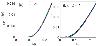
Figure 8: Results of simulated annealing with hopping for HN3. For both (a) and (b), the figure consists of one solid line for the equilibrium result obtained with Wang-Landau sampling and 9 dotted lines obtained with simulated annealing at rates $d\mu=0.001/2^{j}$ for $j=0,\ldots,8$. For HN3 with $l=0$ and $l=1$, the system equilibrates for nearly all annealing schedules, collapsing the data onto the equilibrium line. Only for HN3 with $l=1$, small deviations from equilibrium are observed for annealing schedules $d\mu\gtrsim 10^{-5}$.

III.2.1 Results for HN3

The equilibrium packing fraction and entropy from Wang-Landau sampling as well as the dynamic results from simulated annealing for HN3 are shown in Fig. 6. Based on the analytical results by Boettcher et al. Boettcher and Hartmann (2011), we can confidently conclude that there is no phase transition in HN3 with $l=0$. Yet, the dynamic simulations indicate that the system jams nonetheless. The system jams even further from equilibrium for the case of $l=1$. Here, RG results have not been obtained so far and it is not clear whether there is a thermodynamic phase transition. The equilibrium results from Wang-Landau sampling (at $N=2^{10}$) seem to suggest a singularity near $1/\mu\approx 0.06$ where the entropy density jumps noticeably and $\rho(\mu)\equiv\rho_{CP}$ for all larger $\mu$. Either RG or results for bigger systems may be needed to confirm whether there is phase transition or not.

The possible jamming transitions for both $l=0$ and $1$, revealed by the dynamic annealing simulations in Fig. 6 (a) and (c), are further supported by a power law decay of the residual packing fractions, $\rho_{CP}-\rho^{*}(d\mu)$, as a function of the annealing rate, $d\mu$. Here, we set the jammed packing fraction, obtained at $\mu\to\infty$ after annealing at rate $d\mu$, as $\rho^{*}(d\mu)=\rho(\mu\to\infty;d\mu)$, where $d\mu/dt\to d\mu$ when measured in units of $dt\hat{=}1$ sweep. Note that at these system sizes ($N=32,768$), even the weakest jam is of order $\rho_{CP}-\rho^{*}(d\mu)\approx 0.001$ and, thus, still consists of a sizable number ($\gtrsim 30$) of frustrated particles.

As shown in Fig. 7, a linear fit of the data on a double-logarithmic scale at the largest systems is nearly perfect, justifying the assumption that the time-scales $1/d\mu$ for the existence of the jam diverge asymptotically with a power law for $\rho\to\rho_{CP}$. For HN3 at $l=0$, the slope is $0.34\pm 0.01$ with coefficient of determination $R^{2}=0.9975$, while for $l=1$ the slope is $0.19\pm 0.01$ with $R^{2}=0.9997$, in both cases indicating a dramatic increase of time-scales.

We also test the effect of introducing local hopping, implemented as suggested in step 3 of the algorithm in Sec. II.4, which has not been addressed in Refs. Krzakala et al. (2008); Biroli and Mézard (2002). The results shown in Fig. 8 indicate a substantial difference from the simulation without hopping. For HN3 with $l=0$, the jamming transition disappears even for the fastest annealing schedule, $d\mu=10^{-3}$. For HN3 with $l=1$, the jamming transition can be eliminated at least for an annealing schedule of $d\mu\approx 10^{-5}$ or slower.

Besides the Hanoi networks, we have repeated the annealing simulations on random regular graphs, following Krzakala et al. Krzakala et al. (2008). On those graphs, BM with a hopping dynamics can reach a much denser state than with a varying chemical potential alone, which is similar to what Rivoire et al. Rivoire et al. (2003) argue. But because of the enormous computational cost, we can only test $d\mu$ to as small as $\sim 10^{-6}$ for system sizes at most as large as $\sim 10^{5}$. No results are obtained to conclude that the jamming transition disappears entirely for some smaller $d\mu$, and we suspect that the behavior instead may resemble the mean-field predictions of Rivoire et al. Rivoire et al. (2003).

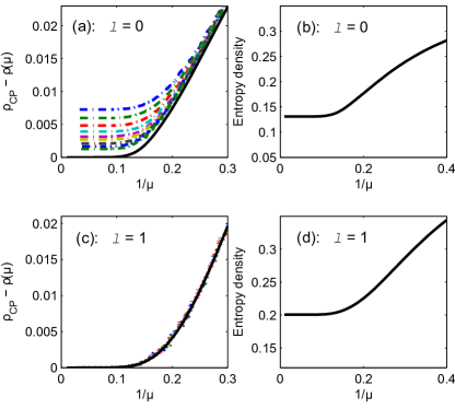
Figure 9: Reduced packing fraction and entropy density for HN5 from Wang-Landau sampling and Simulated Annealing. (a)&(b) are for $l=0$, and (c) &(d) are for $l=1$. The black solid lines represent the equilibrium properties from Wang-Landau sampling with $N=1024$. The dotted lines are from simulated annealing with $N=32,768$, run at different annealing schedules with $d\mu=0.001/2^{j}$ for $j=0,\ldots,8$, from top to bottom. As in Fig. 6, Wang-Landau sampling provides the entropy density via Eq. (2), as shown in (b) and (d).

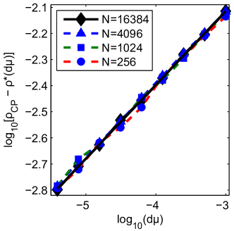
Figure 10: Scaling of the dynamically reached packing fraction $\rho^{*}(d\mu)$ as a function of the annealing rate $d\mu$ for different system sizes $N$ of HN5 for $l=0$, the dashed lines are for systems sizes $N=2^{k}$ with $k=8,10,12$, and 14. All data sets collapse onto the black solid line with a slope of $0.31\pm 0.01$ with $R^{2}=0.9989$, which is obtained from a fit using the data of the largest system size $N=16,384$. Error bars are about of the size of each data point or smaller, indicating a relative error of less than $3\%$.

III.2.2 Results for HN5

The case in HN5 is different from that in HN3. Note that HN5, unlike HN3 and most finite-dimensional lattices or the random graphs studied in Ref.  Krzakala et al. (2008), is not a regular network but has an exponential degree distribution. In HN5 for both, $l=0$ and $l=1$, as shown in Fig. 9, the equilibrium behavior obtained from Wang-Landau sampling is smooth and there is no indication of a phase transition. Annealing reveals a jamming transition and a power law decay similar to that in HN3 in the dynamic simulations only for $l=0$. For $l=1$, surprisingly, there is no jamming transition. The simulations with different annealing schedules equilibrate easily and collapse with the curves from Wang-Landau sampling. This suggests that the combination of heterogeneity in neighborhood sizes together with the possibility to have one occupied neighbor “lubricates” the system sufficiently to avert jams. Correspondingly, the results from Wang-Landau converge rapidly even for larger system sizes. As for HN3, permitting a local hopping dynamics unjams the system also for HN5 with $l=0$.

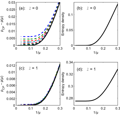
Figure 11: Reduced packing fraction and entropy density for HNNP from Wang-Landau sampling and Simulated Annealing. (a)&(b) are for $l=0$, and (c) &(d) are for $l=1$. The black solid lines represent the equilibrium properties from Wang-Landau sampling with $N=1024$. The dotted lines are from simulated annealing with $N=16,384$, run at different annealing schedules with $d\mu=0.001/2^{j}$ for $j=0,\ldots,8$, from top to bottom. As in Figs. 6 and 9, Wang-Landau sampling provides the entropy density via Eq. (2), as shown in (b) and (d). Note that in the limit of $\mu\to\infty$, HNNP at $l=0$ has a zero entropy which corresponds to a unique ground state. At $l=1$, it attains the same close packing fraction, $\rho_{CP}=\frac{1}{2}$, see Table 1, but now at a non-trivial entropy.

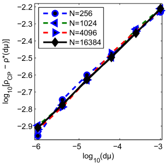
Figure 12: Scaling of the dynamically reached packing fraction $\rho^{*}(d\mu)$ as a function of the annealing rate $d\mu$ for different system sizes $N$ of HNNP for $l=0$, the dashed lines are for systems sizes $N=2^{k}$ with $k=8,10,12$, and 14. All data sets collapse onto the top line with a slope of $0.23\pm 0.01$ with $R^{2}=0.9997$, which is obtained from a fit using the data of the largest system size $N=16,384$. Error bars are about of the size of each data point or smaller, indicating a relative error of less than $3\%$.

Table 2: Summary of the results. For each network, and the allowed neighborhood occupations of $l=0$ and $l=1$, we list to potential for a jam in dynamic simulations and the likely existence of an equilibrium glass transition.

	$l=0$	$l=1$
HN3	Jamming transition & no phase transition	Jamming transition & uncertain
HN5	Jamming transition & uncertain	No jamming transition & no phase transition
HNNP	Jamming transition & uncertain	No jamming transition& no phase transition

III.2.3 Results for HNNP

HNNP provides an interesting alternative among the networks we are considering here. Unlike HN3 and HN5, HNNP is a nonplanar network, but like HN5 it has an exponential distribution of degrees with an average degree of 4. Most importantly, HNNP at $l=0$ possesses a “crystalline” optimal packing that is unique, see Fig. 11(b), and consists of every second site along the line being occupied, i.e., those sites that uniformly have the lowest degree of 3. Therefore, it provides the opportunity to explore the potential for a first-order transition from a jammed state into the ground state, as was observed for lattice glasses in Ref.  Biroli and Mezard (2002). In this case, RG can be applied to obtain $\rho(\mu)$ in equilibrium exactly.

Indeed, we find a weakly jammed state in HNNP with $l=0$, with only a small number of frustrated particles, as shown in Fig. 11. The results of annealing simulations also show a power-law decay (Fig 12), consistent with the approach to a jamming transition. As RG suggest, and the smooth equilibrium curve for $N=1024$ and the convergence with increasing system sizes affirm, there is no thermodynamic phase transition in HNNP with $l=0$. Despite the weakness of those jams, we can find no indication that the annealing simulations at any rate $d\mu$ can ever decay into the ordered state. Apparently, the structural disorder, enforced in HNNP through a heterogeneous neighborhood degree and the hierarchy of long-range links, prevents such an explosive transition. The dominance of such structural elements is further emphasized by the fact that HNNP for $l=1$ exhibits no jams, similar to HN5, with which HNNP shares that structure.

IV Conclusions

We have examined the Biroli-Mezard lattice glass model on hierarchical networks, which provide intermediaries between solvable mean-field models and intractable finite-dimensional systems. These networks exhibit a lattice-like structure with small loops but also with a hierarchy of long-range links imposing geometric disorder and frustration while preserving a recursive structure that can be explored with exact methods, in principle. We observed a rich variety of dynamic behaviors in our simulations. For instance, we find jamming behavior on a regular network for which RG has shown that no equilibrium phase transition exists. However, whether the dynamic transition occurs at a packing fraction distinctly above random close packing remains unclear, and can only be resolved with more detailed RG studies that are beyond our discussion here.

We have simulated the model on our networks with a varying chemical potential $\mu$, with and without local hopping of particles. Hopping impacted those simulations in a significant manner, always eliminating any jams that have existed without hopping. Solutions of the corresponding mean-field systems would have suggested that a dynamics driven by hopping (but at fixed particle number) results in kinetic arrest Rivoire et al. (2003). Whether canonical simulations with hopping alone, or hopping at different rates, would change this scenario, we have to leave for future investigations, as well as the question on whether a combined method of updates would alter the behavior observed on lattices and mean-field networks.

References

- Liu and Nagel (1998) A. J. Liu and S. R. Nagel, Nature 396, 21 (1998).
- Biroli (2007) G. Biroli, Nature Physics 3, 222 (2007).
- Liu and Nagel (2010) A. J. Liu and S. R. Nagel, Annu. Rev. Condens. Matter Phys. 1, 347 (2010).
- Hill and Dissado (1985) R. Hill and L. Dissado, Journal of Physics C: Solid State Physics 18, 3829 (1985).
- Ciamarra et al. (2010) M. P. Ciamarra, M. Nicodemi, and A. Coniglio, Soft Matter 6, 2871 (2010).
- Van Hecke (2010) M. Van Hecke, Journal of Physics: Condensed Matter 22, 033101 (2010).
- Majmudar et al. (2007) T. S. Majmudar, M. Sperl, S. Luding, and R. P. Behringer, Phys. Rev. Lett. 98, 058001 (2007).
- Parisi and Zamponi (2010) G. Parisi and F. Zamponi, Rev. Mod. Phys. 82, 789 (2010).
- Angelani and Foffi (2007) L. Angelani and G. Foffi, Journal of Physics: Condensed Matter 19, 256207 (2007).
- Trappe et al. (2001) V. Trappe, V. Prasad, L. Cipelletti, P. Segre, and D. Weitz, Nature 411, 772 (2001).
- Zhang and Makse (2005) H. Zhang and H. Makse, Physical Review E 72, 011301 (2005).
- Berthier et al. (2011) L. Berthier, G. Biroli, J.-P. Bouchaud, L. Cipelletti, and W. van Saarloos, Dynamical heterogeneities in glasses, colloids, and granular media (Oxford University Press, 2011).
- Da Cruz et al. (2002) F. Da Cruz, F. Chevoir, D. Bonn, and P. Coussot, Physical Review E 66, 051305 (2002).
- Krzakala et al. (2008) F. Krzakala, M. Tarzia, and L. Zdeborová, Phys. Rev. Lett. 101, 165702 (2008).
- Jacquin et al. (2011) H. Jacquin, L. Berthier, and F. Zamponi, Phys. Rev. Lett. 106, 135702 (2011).
- Biroli and Mezard (2002) G. Biroli and M. Mezard, Phys. Rev. Lett. 88, 025501 (2002).
- Kob and Andersen (1993) W. Kob and H. C. Andersen, Phys. Rev. E 48, 4364 (1993).
- Rivoire et al. (2003) O. Rivoire, G. Biroli, O. C. Martin, and M. Mézard, The European Physical Journal B-Condensed Matter and Complex Systems 37, 55 (2003).
- Boettcher et al. (2008) S. Boettcher, B. Gonçalves, and H. Guclu, Journal of Physics A: Mathematical and Theoretical 41, 252001 (2008).
- Boettcher and Hartmann (2011) S. Boettcher and A. K. Hartmann, Phys. Rev. E 84, 011108 (2011).
- Wang and Landau (2001a) F. Wang and D. P. Landau, Phys. Rev. Lett. 86, 2050 (2001a).
- Wang and Landau (2001b) F. Wang and D. P. Landau, Phys. Rev. E 64, 056101 (2001b).
- Boettcher et al. (2009) S. Boettcher, J. L. Cook, and R. M. Ziff, Phys. Rev. E 80, 041115 (2009).
- Lee et al. (2006) H. K. Lee, Y. Okabe, and D. Landau, Computer physics communications 175, 36 (2006).
- Cunha-Netto and Dickman (2011) A. Cunha-Netto and R. Dickman, Computer Physics Communications 182, 719 (2011).
- Kirkpatrick et al. (1983) S. Kirkpatrick, C. D. Gelatt, and M. P. Vecchi, Science 220, 671 (1983).
- Černỳ (1985) V. Černỳ, Journal of optimization theory and applications 45, 41 (1985).
- Biroli and Mézard (2002) G. Biroli and M. Mézard, Phys. Rev. Lett. 88, 025501 (2002).
- Hunter and Weeks (2012) G. L. Hunter and E. R. Weeks, Rep. Prog. Phys. 75, 066501 (2012).