Convergence of quasiparticle self-consistent GW calculations of transition metal monoxides

Abstract

Finding an accurate ab initio approach for calculating the electronic properties of transition metal oxides has been a problem for several decades. In this paper, we investigate the electronic structure of the transition metal monoxides MnO, CoO, and NiO in their undistorted rock-salt structure within a fully iterated quasiparticle self-consistent GW (QPscGW) scheme. We study the convergence of the QPscGW method, i.e., how the quasiparticle energy eigenvalues and wavefunctions converge as a function of the QPscGW iterations, and we compare the converged outputs obtained from different starting wavefunctions. We find that the convergence is slow and that a one-shot G₀W₀ calculation does not significantly improve the initial eigenvalues and states. It is important to notice that in some cases the “path” to convergence may go through energy band reordering which cannot be captured by the simple initial unperturbed Hamiltonian. When we reach a fully iterated solution, the converged density of states, band-gaps and magnetic moments of these oxides are found to be only weakly dependent on the choice of the starting wavefunctions and in reasonably good agreement with the experiment. Finally, this approach provides a clear picture of the interplay between the various orbitals near the Fermi level of these simple transition metal monoxides. The results of these accurate ab initio calculations can provide input for models aiming at describing the low energy physics in these materials.

I Introduction

Transition metal oxides (TMO) form a very interesting class of materials exhibiting a rich variety of physical properties resulting from the interplay of spin, orbital, charge and lattice dynamics. They form the building block of many materials showing complex behavior including superconductivity, colossal magnetoresistance and multiferroic behavior. Among the TMOs, MnO, CoO, and NiO, have been extensively studied, because they are the simplest TMOs with incomplete $d$ shells. Furthermore, they have been used as a playground for applying new ab initio methodology because for some of them, simple density functional theory (DFT) within the local density approximation (LDA) does not yield the correct character of their ground state. While originally they were thought to be Mott insulatorsMott (1949), later studiesTerakura et al. (1984a, b) indicate that these materials might be charge transfer insulators.Zaanen and Sawatzky (1990) These oxides are found in the rock-salt structure in the paramagnetic phase and undergo antiferromagnetic ordering below their Neel temperature along with structural distortions.

Furthermore, understanding these materials is crucial because various applications are being explored using TMOsZhou and Ramanathan (2013), including utilizing their optoelectronic properties.Manousakis (2010); Miller et al. (2012)

The Kohn-Sham DFT within the LDA has provided a very successful ab initio framework to successfully tackle the problem of the electronic structure of materials. However, shortly after the discovery of the copper-oxide superconductors, certain weaknesses of the method were exposed, as it failed to yield the fact that the parent compound La₂CuO₄ is an antiferromagnetic insulator.Pickett (1989) Furthermore, this particular approximation also fails to yield the insulating character of simple $d$ electron transition metal monoxides, such as CoOTerakura et al. (1984b), which is the case of our interest in this paper. This difficult period for the DFT/LDA method was partially ended in the early and mid 90s when an orbital dependent Hubbard type U was incorporated in the exchange correlation functional of the localized $d$ electrons in a mean field fashion within the (LDA) + U methodAnisimov et al. (1991); Liechtenstein et al. (1995), while the itinerant electrons are still described at the LDA level. Although the LDA + U method has been successful in treating localized electron systems, the results are strongly dependent on the choice of the parameter U.

Another approach to the problem is the so called GW approximation of Hedin Hedin (1965) which yields an approximation to the single-particle Green’s function and takes many-body effects into account in the electron-electron interaction. This many-body perturbation technique not only supports a quasiparticle picture, but also accounts for the dynamical screening of the electrons.

This is achieved by approximating the single-particle self-energy as $\Sigma=iGW$, in terms of the single-particle Green’s function $G$ and the dynamically screened Coulomb interaction $W$, which is obtained using the inverse of the frequency-dependent dielectric matrix. In spite of the neglect of vertex corrections in the self energy, which gives rise to higher order correction terms and overestimation of the band gaps due to underestimated dielectric constantsShishkin et al. (2007), the GW calculations give very good agreement between calculated and measured band-gaps (as well as other single-particle properties) for $sp$ semiconductors.van Schilfgaarde et al. (2006); Hybertsen and Louie (1986)

In the case of systems where localized $d$ (or $f$) states are present near the Fermi energy, as in this work, a large number of plane wave states are required to accurately represent these localized states. In order to tackle this problem, Gaussian orbitals or localized basis sets have been used within the linear muffin-tin-orbital (LMTO) methodMethfessel (1988). Such an approach has been repeatedly applied successfully to NiOAryasetiawan and Gunnarsson (1995); Sakuma et al. (2009a), which is a subject of the present paper. There are other methods to circumvent the problem, such as full-potential LMTO or full-potential linear augmented plane-wave methodsAndersen (1975), which use a localized basis set in the muffin-tin region and plane waves in the interstitial region. The projector augmented-wave (PAW) methodBlöchl (1994) as implemented in the VASP codeShishkin et al. (2007); Fuchs et al. (2007); Shishkin and Kresse (2007, 2006) works quite efficiently in conjunction with the GW method.

There is a significant effort to apply the GW approach to the TMOs. There are calculations performed for NiO using the spin-polarized GW approximation in the LMTO basis set Aryasetiawan and Karlsson (1996); Aryasetiawan and Gunnarsson (1995), and a plane-wave basis set with ab initio pseudopotentialsLi et al. (2005). The so-called “model GW” has been used to investigate the single-particle properties of MnO and NiOMassidda et al. (1995) and of MnO, FeO, CoO and NiOYe et al. (2012). All-electron self-consistent quasiparticle GW calculations were performed on MnO and NiOFaleev et al. (2004); van Schilfgaarde et al. (2006). A GW calculationKobayashi et al. (2008) of the single-particle properties starting from LDA+U wavefunctions has been performed on NiO and MnO and a good agreement with experiment was achieved. With a somewhat similar approach, starting from a LDA+U calculation which was followed by G₀W₀ and GW₀ calculations (in which G and W, or just W, is calculated only at the 0th order), the band gap and self-energy of these oxides were also investigatedJiang et al. (2010).

It has been suggested that wave functions obtained within hybrid functional calculations (HSE)Heyd et al. (2003) may provide a good starting point for GW calculationsRödl et al. (2009); Rödl and Bechstedt (2012); Fuchs and Bechstedt (2008). The band structures of MnO, FeO, CoO and NiO have been studied within the HSE+G₀W₀ approach and reasonable agreement with experimental band gaps was foundRödl et al. (2009). However, a recent publicationLany (2013) shows that the choice of HSE functional as the starting wavefunction produces an incorrect band ordering in Cu₂O, which can be resolved by means of a self-consistent GW calculation. Another comprehensive work on hybrid functionals found that the basic HSE06 functional was insufficient for many materials Marques et al. (2011).

Because HSE might be considered a good starting point, one might think that it is sufficient to carry out only a few additional GW iterations. However, it was foundCoulter et al. (2013) that in order to obtain accurate wavefunctions, especially for states near the Fermi energy, one might need to carry out many GW iterations and, thus, this approach is both computationally costly and not parameter free. A recent fully iterated quasiparticle self-consistent GW calculation gives the correct band gap and quasiparticle wavefunctions, independent of the starting LDA and HSE wavefunctions for the transition metal oxide VO₂Coulter et al. (2013). Earlier works using a similar method demonstrated that self-consistency is very important in VO₂Sakuma et al. (2009b, 2008). Additionally, quasiparticle lifetime calculations have been successfully performed in this material by QPscGW, though very high precision is required for such workCoulter et al. (2014).

The method of LDA+DMFT has been consistently useful in the case of strongly correlated TMO’s. It has been fruitful in these materials for many types of study; from accurate electronic and magnetic structureRen et al. (2006); Kuneš et al. (2007a); Thunström et al. (2012); Nekrasov et al. (2013) to exploring metal-insulator transitionsKasinathan et al. (2006); Kunes et al. (2008); Dyachenko et al. (2012) and the effect of dopingKuneš et al. (2007b). As we will discuss in the conclusions section of this paper, these DMFT results associated with character the bands and their ordering near the Fermi level are in agreement with our QPscGW results for the materials we consider in this paper.

In this work we focus our effort to answer a few pressing questions regarding the QPscGW approach to be adopted for later studies of other TMOs: Are too many QPscGW steps required for convergence to make the approach practical? How does the convergence rate depend on the initial quasiparticle wavefunctions, i.e., wavefunctions and energies obtained from a GGA or GGA+U or HSE calculation? How profitable is it to carry out a single shot G₀W₀ calculation on top of GGA, or GGA+U or HSE for this class of materials? How strongly do the converged solutions depend on these initial choices of quasiparticle wavefunctions? Can we approximate the results of the fully converged QPscGW approach with a GGA+U calculation in an appropriate regime of U?

To answer these questions we focus our effort on MnO, NiO and CoO for the following reasons. In the case of MnO and NiO the spin-polarized GGA (sGGA) calculation yields a band-gap. This allows us to start with a QPscGWShishkin et al. (2007); Fuchs et al. (2007); Shishkin and Kresse (2007, 2006) based on wavefunctions and quasiparticle energies obtained by means of a spin-polarized GGA calculation. Similar QPscGW calculations have given good results on similar materialsSvane et al. (2010); Coulter et al. (2013), including strongly correlated $f$ electron systemsChantis et al. (2007, 2008).

However, there are many insulating materials, especially in the class of TMOs, for which a simple sGGA calculation fails to show a gap. CoO is such an example, where sGGA yields no gap. In order to accelerate the rate of convergence of the GW method for CoO, we start the QPscGW iterations using the wavefunctions obtained from a GGA + U calculation. If such calculations are fully iterated, the results should be only very weakly dependent on the initial value of U. In this paper, we have investigated the effect of such starting wavefunctions on the self consistent GW calculations. We explore the convergence with different starting values of U for CoO. For the case of MnO and NiO we explore the convergence starting from wavefunctions and energies obtained from GGA and HSE calculations.

The paper is organized as follows: In Sec. II we discuss the computational approach and the details of the scheme adopted here. In Sec. III we discuss details of the convergence of the QPscGW approach for all three TMOs chosen for the present study. In Sec. IV we present our converged results for bands, gaps, magnetic moment and the density of states for MnO, CoO, and NiO, and we compare them with the experimental results. In Sec. V we discuss the main conclusions of the present study.

II Computational Approach

II.1 The self-consistent GW method

The QPscGW calculations are performed using a variant of the method originally suggested by van Schilfgaarde et al.van Schilfgaarde et al. (2006) as implemented in the VASP code and as outlined in Ref. Shishkin et al., 2007. Notice that the formalism presented in Ref. Shishkin et al., 2007, with the interpretation that the state $n$ is an abbreviation which includes all orbital and spin degrees of freedom, allows us to carry out a QPscGW in which “up” and “down” spin states are handled as in standard spin-polarized DFT. In the current version of the VASP code, the particular vertex correction contribution to the frequency dependent dielectric matrix described in Ref. Shishkin et al., 2007 has not been implemented for the spin polarized case.

In order to perform our QPscGW calculations, we choose a semi-local exchange correlation potential within the sGGA (for MnO and NiO) or the GGA+U (for CoO) approximation as the starting point and we solve the GW equations iteratively as discussed in Ref. Shishkin et al., 2007. The exchange correlation potential is updated at every iteration $i$ by linearizing the self-energy $\Sigma^{(i-1)}(\epsilon)$ obtained in the iteration $i-1$ near the known quasiparticle energy eigenvalue $E^{(i-1)}_{n}$ obtained in the previous step.

$$\textbf{H}^{(i)}\mid\psi^{(i)}_{n}\rangle=E^{(i)}_{n}\textbf{S}^{(i)}|\psi^{(i)}_{n}\rangle,$$ (1)

where the Hamiltonian and overlap matrices are given by:

$$\textbf{H}^{(i)} = T\;+\;V_{ext}\;+\;V_{H}\;+\;V_{xc}^{(i)},$$ (2)

$$V_{xc}^{(i)} = [\Sigma^{(i-1)}(\epsilon)\;-\;\epsilon\frac{\partial\Sigma^{(i-1)}(\epsilon)}{\partial{\epsilon}}]|_{\epsilon=E_{n}^{(i-1)}},$$ (3)

$$\textbf{S}^{(i)} = [1-\;\frac{\partial\Sigma^{(i-1)}(\epsilon)}{\partial\epsilon}|_{\epsilon=E_{n}^{(i-1)}}].$$ (4)

There is no unique method to map this problem onto a corresponding Hermitian eigenvalue problem; the Hamiltonian operator $\textbf{H}^{(i)}$ and the overlap operator $\textbf{S}^{(i)}$ can be expressed in a suitable basis set $|\phi_{n}\rangle$ (e.g., the DFT wave functions), and we take the Hermitian part of the self-energy and overlap matrix in this basisShishkin et al. (2007), i.e., $\tilde{\Sigma}_{mn}\equiv\mathrm{Herm}[\langle\phi_{m}|\Sigma^{(i)}|\phi_{n}\rangle]$ and $\tilde{S}_{mn}\equiv\mathrm{Herm}[\langle\phi_{m}|\textbf{S}^{(i)}|\phi_{n}\rangle]$. Then, the corresponding Hermitian eigenvalue problem

$$\tilde{U}^{\dagger}\tilde{S}^{-1/2}\tilde{H}\tilde{S}^{-1/2}\tilde{U}=\Lambda,$$ (5)

where $\tilde{U}$ is a unitary matrix and $\Lambda$ is the diagonal eigenvalue matrix, in terms of which the updated wavefunctions are given as

$$|\psi^{(i)}_{n}\rangle=\sum_{m}\tilde{U}_{nm}|\phi_{m}\rangle.$$ (6)

These updated energy eigenvalues and the wavefunctions determine the updated Green’s function $G^{(i)}$, i.e.,

$$G^{(i)}(\vec{x},\vec{x}^{\prime},\epsilon)=\sum_{n}\frac{\psi^{(i)}_{n}(\vec{x})\psi^{(i)*}_{n}(\vec{x}^{\prime})}{\epsilon-E^{(i)}_{n}\;\pm\mathit{i}\eta}.$$ (7)

The updated self-energy $\Sigma^{(i)}$ is obtained by convolving the updated Green’s function $G^{(i)}$ with the updated screened Coulomb interaction $W^{(i)}$, i.e.,

$$\Sigma^{(i)}(\vec{x},\vec{x^{\prime}},\omega) = \frac{i}{4\pi}\int_{-\infty}^{\infty}d\omega^{\prime}e^{i\omega^{{}^{\prime}}\delta}G^{(i)}(\vec{x},\vec{x^{\prime}},\omega+\omega^{\prime})$$ (8)

$$\times W^{{}^{(i)}}(\vec{x},\vec{x^{\prime}},\omega^{\prime}).$$

One finds the updated screened Coulomb interaction $W^{(i)}$ using the dielectric function within the random phase approximation (RPA):

$$W^{(i)}(\vec{x},\vec{x^{{}^{\prime}}};\epsilon)=\int d\vec{x}^{{}^{\prime\prime}}\epsilon_{i}^{-1}(\vec{x},\vec{x}^{{}^{\prime\prime}};\epsilon)\textit{v}(\vec{x}^{{}^{\prime\prime}}-\vec{x}^{{}^{\prime}}),$$ (9)

where $\textit{v}(\vec{x}^{{}^{\prime\prime}}-\vec{x}^{{}^{\prime}})$ is the bare Coulomb potential. The dielectric matrix in the iteration $i$ is written as

$$\epsilon_{i}(\vec{x},\vec{x}^{{}^{\prime}};\epsilon)=\delta(\vec{x}-\vec{x}^{{}^{\prime}})-\int d\vec{x}^{{}^{\prime\prime}}\textit{v}(\vec{x}-\vec{x}^{{}^{\prime\prime}})P^{(i)}(\vec{x}^{{}^{\prime\prime}},\vec{x}^{{}^{\prime}};\epsilon).$$ (10)

where in the RPA we simply write that

$$P^{(i)}(\vec{x},\vec{x}^{\prime};\epsilon)=\sum_{n,m}(f_{n}-f_{m}){{\psi^{(i)}_{n}(\vec{x})\psi^{(i)*}_{m}(\vec{x})\psi^{(i)*}_{n}(\vec{x}^{\prime})\psi^{(i)}_{m}(\vec{x}^{\prime})}\over{\epsilon-(E^{(i)}_{m}-E^{(i)}_{n})}+i\eta},$$ (11)

where $f_{n}=F(E^{(i)}_{n})$ and $f_{m}=F(E^{(i)}_{m})$ and $F(E)$ is the T=0 Fermi-Dirac distribution.

II.2 Computational Details

All the computations were performed using the Vienna Advanced Simulation Package (VASP)Shishkin et al. (2007); Fuchs et al. (2007); Shishkin and Kresse (2007, 2006). The Perdew-Burke-Ernzerhof (PBE) exchange correlation functionalPerdew et al. (1996) was used for all GGA calculations. The GGA+U calculations were done using the Dudarev approachDudarev et al. (1998) where the difference of U and J is incorporated in the calculation as an effective U. The 4s and 3d electrons of the transition metal atom and the oxygen 2s and 2p electrons were treated as valence electrons. The projected augmented wave (PAW) methodologyBlöchl (1994) was used to describe the wavefunctions of the core electrons. The electronic wavefunctions were described by plane waves, where energy cutoff of 315 eV (MnO), 500 eV (CoO), and 400 eV (NiO) were used for all GGA and GW calculations.

The Brillouin zone was sampled with a $4\times 4\times 4$ k-point meshMonkhorst and Pack (1976) and a maximum of 144 bands and 88 bands were used for the GGA and GW calculations. This size of k-point mesh is acceptable for this type of study, as the quasi-particle energy convergence does not depend strongly on the k-point setKlimeš et al. (2014).

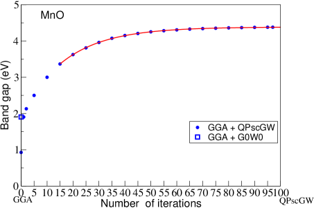
Figure 1: (color-online) The band-gap as a function of the QPscGW iterations. The starting wavefunction comes from a GGA calculation.

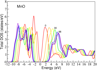
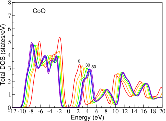
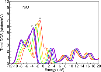
Figure 2: (color-online) Convergence of the DOS as a function of the number of iterations for MnO (starting from GGA), CoO (starting from GGA+U with U=3 eV), and NiO (starting with GGA). The curves are labeled by some selected iteration numbers to guide the eye of the reader.

Recently, the convergence of G₀W₀ calculations has been studied with respect to number of bands and number of plane waves in the response function basisKlimeš et al. (2014). This study also points out some convergence problems with using non-norm-conserving pseudopotentials in the PAW methods. However, the current PAW pseudopotentials available are only of this type, We can only compare our results in this section to the results presented in that work with non-norm-conserving pseudopotentials. Accordingly, we have checked this using MnO and NiO as examples. In MnO, we find that increasing the number of conduction bands from 35 to 227 the direct band gap at $\Gamma$ in G₀W₀ changes by only 0.04 eV from 2.44 eV to 2.40 eV. In the case of NiO, we find that going from 66 to 478 conduction bands makes only a 0.05 eV difference in the gap. In the aforementioned study, the difference was far more striking in the test material ZnO; the same amount of change in number of bands showed a 0.2 eV difference in the gap. We suspect ZnO to be somewhat extreme in this regard. The previous study primarily showed change in the absolute energy levels, which we are not concerned with here. For the response-function basis set in the case of MnO by keeping the number of bands fixed and increasing the energy cutoff from 200 eV ($\sim 300$ plane waves) to 600 eV ($\sim 1500$ plane waves) we find that the direct gap at $\Gamma$ only changes from 2.44 eV to 2.46 eV. All of these corrections are quite small compared to the huge changes we find as a result of using QPscGW vs. G₀W₀.

All of the chosen materials crystallize in the rock salt structure. Small low temperature distortions from the cubic structure have been ignored in these calculations. In other work on MnO, this was found to have little to no effect on the electronic spectrumTomczak et al. (2010). The most stable antiferromagnetic (AF II) state has been used, with the magnetization along alternate [111] planes. The lattice constants taken from experimental results as: 8.863 $\AA$ (MnO)Cheetham and Hope (1983), and 8.380 $\AA$ (NiO)Rooksby (1948). For the case of CoO we used a value of 8.499 $\AA$ taken from Ref. Rödl and Bechstedt, 2012 which was determined such that the volume of the (doubled) cubic unit cell to coincide with the volume of the distorted unit cell as determined experimentallyJauch et al. (2001). This value does not exactly coincide with the experimental value of 8.521 $\AA$Jauch et al. (2001) for CoO. For the case of the other two compounds the experimental values of the lattice constant and those determined in order to keep the volume of the cubic unit cell the same as the distorted unit cell are very close. In all three cases, we use the rhombohedral primitive cell in our calculations. All reciprocal lattice points are given in the basis of the corresponding reciprocal vectors.

For the GW calculations we have used a $4\times 4\times 4$ k-point mesh and a maximum of 88 bands. We used 64 values of omega in the evaluation of the response functions.

III Study of Convergence

III.1 Convergence study in MnO

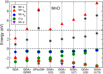
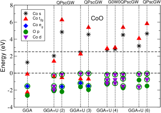
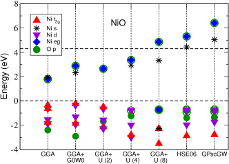
Figure 3: (color-online) We present the character of the bands nearest to the Fermi level at the $\Gamma$ point for MnO, CoO and NiO, for different types of calculation. The various symbols shown in the figure legends correspond to the indicated orbital content. When multiple symbols are used for the same band, it means that the orbital content of that particular band is a mixture of the orbital with the corresponding overlapping symbols. Where we find clearly separated $t_{2g}$ and $e_{g}$ states, we mark them accordingly; where the states of those characters are mixed, we label them $d$ states. We present the quasiparticle energies for a few bands above and below the “Fermi energy” (the valence band edge is shifted to be 0 eV) as obtained by GGA+U approximation with various values of U, and by the fully iterated QPscGW calculations. The horizontal bottom and top axes are used to indicate the approximation level. The vertical axis is used for the quasiparticle energies.

We start our QPscGW calculation with the wavefunctions obtained from an sGGA calculation for MnO. The convergence of the gap as a function of iterations is shown in Fig. 1. Notice that the convergence is monotonic but slow, and it takes about 80 iterations for convergence. We used the following simple expression

$$\Delta_{n}=\Delta_{\infty}-A\exp(-{n\over{\tau}}),$$ (12)

to fit the dependence of each gap value $\Delta_{n}$ on the iteration $n$. The lines through the calculated points are the results of applying this fitting procedure. This procedure gives an estimate of the gap extrapolated to infinite $n$, i.e., the fitting parameter $\Delta$. For the case of MnO we find that $\Delta_{\infty}$=4.39 eV which is very close to the value of our last iteration (i.e., $n=98$); at $n=98$ we found $\Delta_{98}=4.38$ eV, which indicates that our QPscGW scheme has converged.

We would like to stress that a single-shot G₀W₀ calculation, shown in Fig. 1 by an open circle, is not nearly sufficient to bridge the difference between the gap obtained within GGA (0.9 eV) and the converged QPscGW gap (4.38 eV). The G₀W₀ calculation yields a gap of approximately 1.9 eV which is small compared to the fully converged value of 4.38 eV. As we will discuss later in the case of NiO, even a G₀W₀ on top of HSE gives a fraction of the correction needed to bridge the difference between the gap obtained at the HSE level and that obtained at the fully converged stage.

Fig. 2 illustrates the convergence of the density of states as a function of the QPscGW iteration for MnO using quasiparticle wavefunctions obtained from a GGA calculation.

In Fig. 3 we present the character of the bands nearest to the Fermi level for MnO and its comparison to the GGA+U calculations. It will be discussed in Sec. IV in detail.

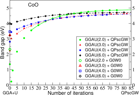
Figure 4: (color-online) CoO: Convergence of the band-gap as a function of QPscGW iterations.

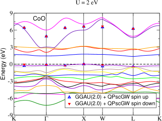
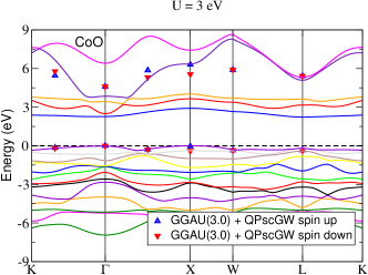
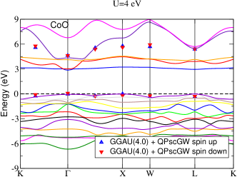
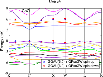
Figure 5: (color-online) The energy bands of CoO near the Fermi level as obtained from a GGA+U calculation with U=2,3,4 and 6 eV (solid lines). The lowest conduction and highest valence bands obtained from the fully converged QPscGW calculation based on the various values of U are also shown by different symbols. Bands are colored only to aid the eye; the color scheme for each material is consistent throughout.

III.2 Convergence study in CoO

For CoO the sGGA approach fails to yield a non-zero band-gap, which indicates that the measured gap in CoO may be due to strong correlations.

Let us consider the fully converged solution $G^{*}$ obtained for the one-particle Green’s function corresponding to the GW equation as the fixed point of an iterative scheme in which we start from a given $G_{0}$ and from any $G_{n}$ we obtain the $G_{n+1}$, etc. This fixed point, if it exists, should be insensitive to the starting $G_{0}$, assuming that every $G_{0}$ used is analytically connected to the same phase. In order to apply many-body perturbation theory as well as reduce the computational cost of the GW calculation, it is important to start with a wavefunction close to the converged solution. Following these two principles in the case of CoO, we begin the iterative QPscGW calculation using wavefunctions obtained from a GGA + U calculation. We will show that because our calculation is fully converged, the results are only weakly dependent on the initial value of U. So, we perform the QPscGW calculations based on wavefunctions calculated with a range of values for U from 2.0 to 6.0 eV.

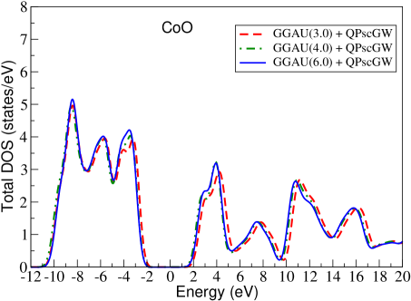
Figure 6: (color-online) Comparison of the DOS for the converged solutions starting from the results of GGA+U calculations with U=3, 4 and 6 eV.

Recent constrained RPA calculationsSakuma and Aryasetiawan (2013); Miyake et al. (2009); Sasioglu et al. (2011) as well as other approachesCococcioni and deGironcoli (2005); Pickett et al. (1998) suggest that the value of U for a simple GGA+U calculation should be around 3 eV. The energy gap obtained from the QPscGW procedure as a function of the iteration number is presented in Fig. 4. The solid lines through the data points are fits obtained using the formula given by Eq. 12, which yields the following values for the extrapolated gaps: 4.91, 4.66, 4.65, and 4.73 eV for U=2,3,4, and 6 eV respectively. Notice that while the starting gaps for the different values of U vary by about 2 eV, the converged values of the gaps are about the same and fall in the range of 4.65 eV to 4.9 eV Thus, the estimated gap is $4.78\pm 0.13$ eV, which provides an estimate of the systematic error of our QPscGW approximation in this case. As we will discuss below, the accumulated error from omitting vertex corrections, from finite size k-point mesh, and from limiting the number of bands, etc, we believe, is larger than this value.

In Fig. 5 we present the calculated band structure for the four different cases. Fig. 5, Fig. 5, Fig. 5, and Fig. 5 correspond to the results of the fully converged QPscGW calculation starting from GGA+U calculations with U=2 eV, 3 eV, 4 eV, and 6 eV respectively. The results of the corresponding starting GGA+U calculations are shown in each figure with the solid lines and the fully converged QPscGW results for the highest occupied and the lowest unoccupied bands are shown by up-triangles (spin up) and down-triangles (spin down).

First, notice that while the starting bands are very different for the four different starting GGA+U calculations, the final QPscGW results are very close to each other. Second, notice that the valence band of the QPscGW calculation is similar to the simple GGA+U calculations. Notice also in Fig. 3 that the ordering of the valence bands near the Fermi energy for CoO as obtained from GGA+U calculations is similar to that obtained from the corresponding QPscGW calculations. The third very important conclusion of this calculation is, however, that the conduction band obtained from the QPscGW calculation closely resembles the features of the GGA+U calculation for U = 4 eV and U = 6 eV. Namely, the results at the GGA+U level show band crossing and hybridization in the vicinity of the $\Gamma$ point as a function of U.

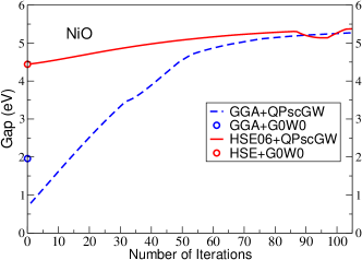
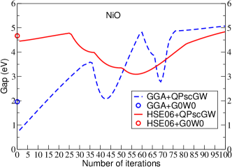
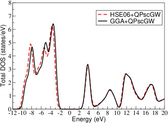
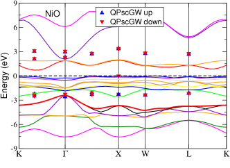
Figure 7: (color-online) NiO: (a) Convergence of the band gap for spin-up electrons with iterations starting from GGA and HSE wavefunctions. (b) Convergence of the band gap between spin-up and spin-down electrons with iterations starting from GGA and HSE wavefunctions. (c) Comparison of the converged density of states obtained after QPscGW calculations starting from HSE06 and sGGA. (d) Illustration of the “level crossing” state at the 43rd step of the QPscGW procedure in which a spin-down state temporarily moves to a higher energy, decreasing the gap. Bands are colored only to aid the eye; the color scheme for each material is consistent throughout.

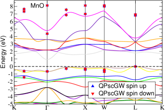
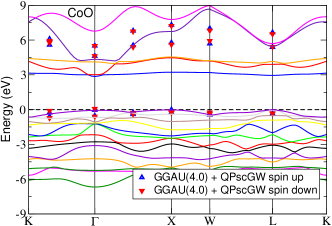
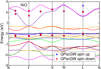
Figure 8: (color-online) The bands obtained (a) for MnO using sGGA (solid lines) and fully converged QPscGW (open or full circles), (b) CoO using GGA+U (solid lines) and fully converged QPscGW (open or full circles), and (d) for NiO using sGGA (solid lines) and fully converged QPscGW (open or full circles) Bands are colored only to aid the eye; the color scheme for each material is consistent throughout.

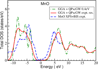
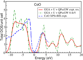
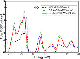
Figure 9: (color-online)The density of states of transition metal oxides MnO, NiO, and NiO obtained by solving the GW equations self-consistently is compared to the experimental XPS and BIS data.van Elp et al. (1991a, b); Sawatzky and Allen (1984)

The hybridization starts at U$\sim 4$ eV and involves one dispersionless lower energy band of Co $t_{2g}$ character and one higher energy, strongly dispersive Co $s$ band. The result of the hybridization is to produce a conduction band which is dispersive only near the $\Gamma$ point where the hybridized lower energy band inherited the dispersion from the $s$ band. This behavior also occurs in the transition at around U = 4 eV seen in the level ordering of the lowest two conduction bands in Fig. 3. This is the exact same character as the lowest conduction band obtained as the final result of the QPscGW iterations independently of the starting wavefunctions. Namely, the result of the QPscGW calculations and that of the simple GGA+U calculations above U$\sim 4$ eV are qualitatively very similar and the main difference is in the size of the gap.

It is important to discuss some additional details of our results. Notice that the energies of the converged QPscGW states having different spins, with all other quantum numbers common, are somewhat different. The reason is that the energy levels for up and down spins are free to vary independently in the present QPscGW calculations. As we will discuss in the case of NiO this effect becomes more pronounced there. The departure from up-down symmetry is temporarily explored by the QPscGW iteration procedure as a possible path to reaching a fully converged solution; however, it seems that the final fully converged solution is the up-down symmetric one.

We have noticed that during the QPscGW evolution from the starting to the final state, level crossings have occurred in all four cases. Starting with U=3 eV, for example, the conduction band minimum for spin-up, obtained from the initial GGA+U calculation, is at $\vec{k}=(1/2,1/2,1/2)$ (in units of the reciprocal lattice vectors of primitive unit cell of the rock-salt structure), while the converged QPscGW calculation yields a conduction band minimum at the $\Gamma$ point. Furthermore, in general, we find that the orbital ordering, as well as the exact $\vec{k}$ point where the valence band maximum occurs, may be slightly different for the converged states for different values of U. These discrepancies between the character of the converged states starting from different values of U may be due to the following reasons:

a) The lowest conduction band, as well as the highest valence band, have a narrow bandwidth, consistent with the belief that CoO is a strongly correlated material with nearly localized electrons near the Fermi level. Therefore, the energy eigenvalues corresponding to various values of $\vec{k}$ are different by a very small amount which may be beyond the level of accuracy of the present QPscGW calculation. This is illustrated in Fig. 5.

b) When level crossing occurs, during the QPscGW evolution, the adiabatic nature of such an evolution can not be guaranteed. Namely, the adiabatic theorem states that: in a real-time evolution is adiabatic, i.e., in order for the eigenstates found by solving the time-dependent Schrödinger equation to be in one-to-one correspondence with the starting eigenstates and to correspond to the eigenstates of the perturbed instantaneous Hamiltonian there must be no level crossing during the time-evolution.

c) We found that already, at the GGA+U level, there is such a level crossing as a function of $U$. For example, the valence band maximum for U=2 eV occurs at $\vec{k}=(0,1/2,1/2)$, while for U=6 eV it occurs at $\vec{k}=(1/2,1/2,1/2)$. Therefore, starting from unperturbed Hamiltonians corresponding to such different values of U, the QPscGW is forced to evolve through at least one level crossing in order to reach the same solution at the converged stage. Fig. 5 demonstrates the band crossing which happens at the GGA+U level. The lowest conduction band, which is nearly dispersionless and of Co $t_{2g}$ character at $\Gamma$, hybridizes near $\Gamma$ with another band of pure $s$ character, as we increase the value of U from 3 to 4 eV.

More general features such as the converged QPscGW density of states, obtained with different starting wavefunctions, agree with each other quite nicely. Fig. 2 illustrates the convergence of the density of states as a function of the QPscGW iteration for CoO using quasiparticle wavefunctions obtained from a GGA+U calculation with U = 3.0 eV. Here, we begin with a gap of 2.23 eV at the GGA+U level with U = 3.0 eV. After 80 iterations, where convergence is achieved, and using the extrapolation discussed in the previous subsection we obtained a gap of 4.66 eV.

In Fig. 6, we show that starting with wavefunctions obtained from different GGA+U calculations with U = 3.0, 4.0 and 6.0 eV the QPscGW procedure converges to very similar density of states. Although the GGA+U band gaps with U = 3.0, 4.0 and 6 eV differ by 2.0 eV, the final QPscGW calculations converge to similar density of states and similar gaps with a spread of $\pm 0.13$ eV. This indicates that these QPscGW calculations are to a certain degree weakly dependent on the choice of the starting wavefunctions within the regime of perturbation theory.

III.3 NiO: Starting with GGA, and HSE

It has been claimed that although QPscGW results may be preferable, they are computationally very costly, thus, using starting wavefunctions obtained from hybrid functionals such as the HSE Heyd et al. (2003), followed by a single shot GW calculations may be a good practical alternativeRödl et al. (2009). However, the suitability of this approach for TMOs was recently questionedCoulter et al. (2013), namely, whether or not we can just stop at low order in a GW approach having started the GW calculation from wavefunctions and quasiparticle energies obtained from such an HSE calculation.

In Fig. 7, we present the results of two different QPscGW calculations, one starting from GGA and a second starting from the HSE06 functional. This figure shows the gap for up-spin states. First, it appears that both calculations converge smoothly. Notice that the result of the G₀W₀ on top of either GGA or HSE06 makes a small improvement towards the fully converged value of the gap.

On the other hand, however, in Fig. 7 we present the absolute energy gap, namely, the energy difference between occupied and unoccupied states independently of the spin character of the band. Notice that both calculations, much before they take a “path” to final convergence, depart significantly from the original values of the gap. The reason is that the energy levels for up and down spins are free to vary independently in the present QPscGW calculations. As a result, at the iteration where the gap deviates from the monotonically increasing behavior, we find that the down-spin energy eigenvalue which corresponds to the valence band at the X point ($k=(1/2,0,1/2)$) starts rising, thus, entering “inside” the gap leading to level crossing. This is illustrated in Fig. 7, where we plot the bands at the 43^rd QPscGW iteration at which the energy of the top-most valence band for the down-spin state at the X point rises. This is a somewhat similar behavior to that discussed in the case of CoO. Eventually, as the QPscGW iteration process continues, this energy level is lowered again and the QPscGW procedure converges.

In Fig. 7 we compare the converged density of states obtained from the QPscGW calculations starting from HSE06 and sGGA. Notice that the agreement is very good. As we will see in the following section, the converged solution for the density of states compares rather well with the experimental photoemission results.

III.4 Self-energy and spectral functions

In Fig. 10(a-c) we present the calculated real and imaginary parts of the self-energy at the $\Gamma$ point for the highest valence band (circles joined by blue lines) and the lowest conduction band (square joined by red lines). The intersection between the the 45^∘ sloped green dashed-line and the $Re\Sigma$ yields the value of the on-shell value of the real-part of $\Sigma$. Notice that, the imaginary part of $\Sigma$ is small for values of $\omega$ near the quasiparticle peaks. In Figs. 10,10,10 the imaginary part of the Green’s function at the $\Gamma$ point is presented for the lowest conduction band (squares joined by red lines) and the topmost valence band (circles joined by blue lines). In addition, the imaginary part of $G$ is plotted for the same bands that are shown in Fig. 3. All curves scaled down by a factor of 50 are also plotted. Notice that the half-width at the quasiparticle peaks is small and it is the imaginary part of the self-energy at the quasiparticle peak. This indicates that a) the quasiparticle states are relatively well-defined near the QP peaks, and b) neglecting the imaginary part of $\Sigma$ in Eq. 2, and Eq. 3, may be a justified approximation for these materials.

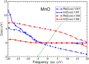
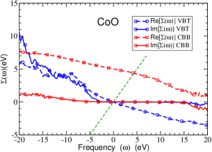
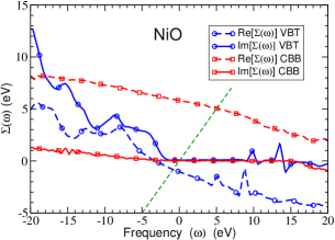
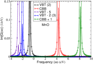
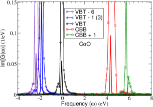
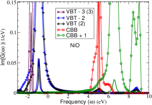
Figure 10: (color-online)Top: The real and imaginary parts of the self-energy are shown for the three TMOs for the topmost valence band (VBT) and the lowest conduction band (CBB) at the $\Gamma$ point. Bottom: The imaginary part of $G$ for the VBT (circles joined by blue lines) and for the CBB (circles joined by blue lines) at the $\Gamma$ point. In addition, the imaginary part of $G$ for a few other bands are shown. These curves are labeled as CBB+n or VBT-n, where $n$ denotes the order of the band above or below the lowest conduction or highest valence band respectively. The degeneracy of each state is given in parentheses if it is different from 1. Under each curve the same curves are plotted in plain solid lines and scaled down by a factor of 50.

IV Fully Converged QPscGW Results

IV.1 Bands, gaps and magnetic moments

In Fig. 8, the bands for MnO, CoO, and NiO are shown, as obtained from sGGA or GGA+U (solid lines) and from QPscGW (up and down triangles). The bands slightly break the up-down symmetry as discussed in Section III.

In MnO, CoO and NiO, the conduction band minimum(CBM) at the $\Gamma$ point is found to be of purely $s$ character. In the conduction band, as we move away from the $\Gamma$ point, we find a significant contribution from the Mn $t_{2g}$ states and Ni $e_{g}$ states in the case of MnO and NiO respectively. For CoO, the character of the conduction band changes from $s$ to Co $t_{2g}$ as we move away from the $\Gamma$ point.

In the case of MnO and NiO, the valence band maximum (VBM) is dominated by transition metal $e_{g}$ states along with some mixture of O $p$ states. In CoO, the VBM has mostly Co $t_{2g}$ character with considerable admixture of $e_{g}$ states and hybridized with O $p$. As is apparent from Fig. 8, the bands near the Fermi energy of all three materials are very flat, which makes it difficult to determine the exact nature of the VBM within the accuracy of the QPscGW calculation.

In Fig. 3 the band order for MnO at the $\Gamma$ point is given for sGGA, and for GGA+U with various values of U, along with the results of our QPscGW calculation starting from sGGA. Notice that as a function of U, the GGA+U calculation leads to the same band-type ordering as sGGA for states near the Fermi level, except for large values of U (7 eV) where another $s$-type band with some O $p$ admixture comes into play. The same $s-p$ band appears in the converged state of the QPscGW calculation as shown in Fig. 3. Since this behavior appears in the GGA+U calculation for large U, it can be understood in the following way. At such high values of U, in the GGA+U calculation the large on-site Coulomb repulsion separates the energy eigenvalues of the $t_{2g}$ from the $e_{g}$ states, such that the O $p$ state surfaces and mixes with a significant portion of the Mn $e_{g}$ state to form the top valence band. For the same reason, the conduction band of $s-p$ character comes down because the $t_{2g}$ states are pushed up. For significantly greater values of U (15 eV) the topmost valence band becomes a pure O $p$ band and the $t_{2g}$ conduction band is pushed even higher. Therefore, we conclude that a simple GGA+U calculation qualitatively describes the orbital content of the bands near the Fermi level in MnO at the $\Gamma$ point. We should stress, however, that in this regime, where the orbital character between QPscGW and GGA+U match, the band-gaps do not match in size. The value of the gap obtained for GGA+U with U=7 eV is 2.35 eV and the gap obtained with QPscGW is $\sim$ 4.4 eV. However, if one forces GGA+U to describe the correct size of the gap by choosing an approximate value of U, then one gets into a regime with the wrong orbital content near the Fermi energy.

The nature of the lowest conduction bands and the highest occupied bands for the case of CoO has been discussed thoroughly in Sec. III. The reader is referred to that section for the illustration of the interesting physics arising from the hybridization and the interplay between the lowest conduction band, which is of Co $t_{2g}$ character and is almost dispersionless, and the next lowest but much more dispersive conduction band, which is of Co $s$ character. This hybridization gives rise to dispersion in the vicinity of the $\Gamma$ point. As mentioned in Sec. III, this hybridization occurs as a function of U in the GGA+U approximation for values of U $>$ U_c (where U_C is between 3 and 4 eV). The physics of the actual material, CoO, resides in the regime of U $>$ U_c. Again, we want to stress that, while the physics of CoO as seen by the fully convergent QPscGW calculation and the GGA+U is similar, in the regime of U where this happens, the size of the GGA+U band gap is significantly smaller than the QPscGW gap.

Fig. 3 illustrates that the level ordering of NiO, as obtained by the fully converged QPscGW calculation starting from either GGA or HSE06, is the same as that obtained by the HSE06 calculation. The conduction band ordering is also similar to that obtained by the GGA+U calculation. The nature of the highest valence bands obtained by GGA+U for U = 4 eV is similar to the QPscGW results for two of the three topmost Ni valence bands of $d$ character at $\Gamma$. If we increase the value of U to 8 eV, the nature of the topmost valence bands becomes O $p$ type at the $\Gamma$ point, which is qualitatively different from the character of these bands obtained from the QPscGW calculation. The reason for this may be the fact that a large value of U pushes the Ni $d$ states away from each other, which brings the O $p$ states to the surface because they are not affected by the large value of U.

Gap (eV)	MnO	CoO	NiO
GGA (indirect)	0.9	0.0	0.7
GGA+U (U=4 eV) (indirect)		2.81	—
HSE03 (indirect) Rödl et al. (2009)	2.6	3.2	4.1
HSE03 (direct) Rödl et al. (2009)	3.2	4.0	4.5
HSE03+G0W0 (indirect) Rödl et al. (2009)	3.4	3.4	4.7
HSE03+G0W0 (direct) Rödl et al. (2009)	4.0	4.5	5.2
QSGW (indirect) van Schilfgaarde et al. (2006)	3.5	—	4.8
mGW (indirect) Ye et al. (2012)	4.03	3.02	3.6
LDA+U+GW (indirect) Jiang et al. (2010)	2.34	2.47	3.75
Present QPscGW (indirect)	4.39	4.78$\pm$0.13	5.0
Photoemission	3.9$\pm$0.4van Elp et al. (1991a)	2.5$\pm$0.3van Elp et al. (1991b)	4.3Sawatzky and Allen (1984)
Conductivity	4.0$\pm$0.2Drabkin et al. (1968)	3.6$\pm$0.5Gvishi and Tannhauser (1972)	3.7Iskenderov et al. (1968)
Optical Absorption	3.7$\pm$0.1Iskenderov et al. (1968)	2.8Pratt and Coelho (1959), 5.43Kang et al. (2007)	3.7Powell and Spicer (1970), 3.87Kang et al. (2007)

Table 1: Comparison of the energy band gaps as obtained in the present work with other methods along with various experimental results.

Moment ($\mu_{B}$)	MnO	CoO	NiO
GGA	4.34	2.4	1.3
GGA+U (U=4 eV)		2.73
HSE03Rödl et al. (2009)	4.5	2.7	1.6
QSGWvan Schilfgaarde et al. (2006)	4.8	—	1.7
mGWYe et al. (2012)	4.56	2.61	1.57
Present (QPscGW)	4.58	2.74	1.7
Experiment	4.58Cheetham and Hope (1983)	3.35Khan and Erickson (1970), 3.8Roth (1958),Herrmann-Ronzaud et al. (1978), 3.98Jauch et al. (2001)	1.9Cheetham and Hope (1983),Roth (1958)

Table 2: Comparison of the magnetic moments as obtained in the present work with other methods along with various experimental results.

In Table 1, the band gaps obtained from our QPscGW approach are compared with various other parameter-dependent and ab initio methods. For MnO, we started with a gap of 0.9 eV obtained from an sGGA calculation and the converged QPscGW calculation yields a gap of 4.39 eV, which is somewhat larger than but in reasonably good agreement with the observed photoemission results within experimental error. For NiO, the band gap obtained by our calculations is 5.0 eV, which is somewhat larger than the experimental value of 4.3 eV. For CoO, our QPscGW calculations starting with wavefunctions and quasiparticle energies obtained from a GGA+U with U = 2, 3, 4 or 6 eV, yield a band gap of 4.78$\pm 0.13$ eV. This band-gap also overestimates the experimental gap. Therefore, we find a systematic overestimation of the band-gaps of these TMOs. This is expected due to the missing vertex correctionsShishkin et al. (2007) and reduced quasiparticle screening.

We would also like to note that our results concerning the band character and ordering are in excellent agreement with those from LDA^′+DMFTNekrasov et al. (2013), as can be inferred from the projected density of states and band structures given in the work cited above.

In Table 2, the local magnetic moments of MnO, CoO and NiO are compared with their values obtained using different approaches. The calculated magnetic moment for MnO using the QPscGW method is in excellent agreement with experimental value. The value of the moment obtained for CoO is significantly lower than the experimental value and this may be attributed to the orbital contribution to the magnetic moment.Rödl et al. (2009) Calculations at the GGA+U level including the orbital contribution significantly increases the moment to 3.58, which is within the range of experimentally obtained values.

IV.2 Density of states

Fig. 9 shows the self-consistently converged density of states for these TMOs as compared to experimental photoemission experiments. The center of the gap of the experimental photoemission data is aligned with that of the calculated density of states. The dot-dashed lines are the calculated DOS where a Gaussian broadening with 0.4 eV full-width has been applied. The solid lines correspond to the calculated DOS where a Gaussian broadening with the experimental resolution has been applied. The experimental resolution depends on both material and XPS vs BIS measurements. These are taken directly from the corresponding references for each of the materialsvan Elp et al. (1991a, b); Sawatzky and Allen (1984). In addition, we have scaled the intensities of the XPS and BIS separately to approximately mimic the amplitudes of the DOS. Notice that the experimental resolution for both XPS and BIS is poor ($\sim 1eV$) and, thus, determining the size of the gaps (given in Table 1) and the location of the Fermi level is difficult. Thus, instead of aligning the experimental and calculated Fermi levels we chose to align the center of the gaps. The density of states is in reasonable overall agreement with the intensity of the experimental XPS and BIS data. The QPscGW calculation leads to an overestimation of band-gaps due to the neglect of the vertex corrections in the GW approximationShishkin et al. (2007); van Schilfgaarde et al. (2006).

V CONCLUSIONS AND SUMMARY

We have studied the electronic structure of the $d$ electron systems MnO, CoO, and NiO by means of the QPscGW approach with the aim to answer the convergence questions outlined in the Introduction of this paper.

First, we studied the convergence of the QPscGW procedure starting from GGA+U with different values of U. Using a rather wide range of values of U (2-6 eV) for CoO, we find that our converged results for bands and density of states are weakly dependent on the starting GGA+U solutions. The fully converged energy bands and density of states, starting from different values of U, are very close to each other. In addition, we found that starting our QPscGW procedure from GGA+U wavefunctions and eigenvalues can improve the convergence if a suitable value of U is chosen.

We also studied the convergence of QPscGW for NiO starting from HSE06 quasiparticle states and from quasiparticles as obtained from an sGGA calculation. We find that the results for the bands and the density of states are in very good agreement with each other. Interestingly, we find that during the QPscGW evolution towards the converged solution, certain levels cross and this makes the “path” temporarily diverge from the approach to the converged solution.

We find that single-shot G₀W₀ calculations are somewhat insufficient to bridge the difference between the gap obtained within any of the starting states (including when we start from HSE) and the converged QPscGW gap. Namely, even a G₀W₀ on top of HSE gives only a fraction of the correction needed to bridge the difference between the gap obtained at the HSE level and the gap obtained at the fully converged level.

This convergence study as a function of U also demonstrates that the physics of CoO for the bands near the Fermi level is very similar to that obtained from a GGA+U calculation for values of U above 4 eV where a hybridization occurs between a lower energy dispersionless conduction band of Co $t_{2g}$ character and a much more dispersive Co $s$ band.

For the case of MnO, we find that within a simple GGA+U treatment, there is a region of U where the orbital character of the bands near the Fermi level and their relative ordering, as obtained by the fully converged QPscGW approach, can be reproduced. For NiO, the band ordering near the Fermi level obtained by the QPscGW calculation can only be partially described by means of a simple GGA+U calculation using a U only on the $d$ levels.

The magnetic moments obtained by solving the GW equations self-consistently agree reasonably well with experimental results. The calculated band-gaps are somewhat overestimated as expectedShishkin et al. (2007); Faleev et al. (2004) due to reduced quasiparticle screening and neglect of vertex corrections. Furthermore, the calculated density of states, determined from the converged wavefunctions and quasiparticle energies, agrees reasonably well with the results of photoemission experiments. We have also shown that the self-consistently determined wavefunctions and energy gaps are weakly dependent on the starting wavefunctions.

We conclude that this approach to transition metal oxides with $d$ states at the Fermi level may be computationally demanding, but it is a genuinely parameter-free approach and provides a good prediction for energy gaps, magnetic moments, density of states, and quasiparticle wavefunctions. In addition, such an approach is quite important for testing the simpler picture suggested from GGA+U calculations and can provide useful input for model studies aiming at describing the low energy physics in these materials.

We believe that an improvement of the approach could be made by generalizing the approach suggested in Ref. Shishkin et al., 2007 and Ref. Faleev et al., 2004 to include vertex corrections for spin-polarized systems.

VI Acknowledgments

This work was supported in part by the US National High Magnetic Field Laboratory, which is partially funded by the US National Science Foundation.

References

- Mott (1949) N. F. Mott, Proceedings of the Physical Society of London Series A 62, 416 (1949).
- Terakura et al. (1984a) K. Terakura, A. R. Williams, T. Oguchi, and J. Kubler, Phys. Rev. Lett. 52, 1830 (1984a).
- Terakura et al. (1984b) K. Terakura, T. Oguchi, A. R. Williams, and J. Kubler, Phys. Rev.B 30, 4734 (1984b).
- Zaanen and Sawatzky (1990) J. Zaanen and G. A. Sawatzky, J. Solid State Chem. 88, 8 (1990).
- Zhou and Ramanathan (2013) Y. Zhou and S. Ramanathan, Journal of Applied Physics 113, 213703 (pages 12) (2013).
- Manousakis (2010) E. Manousakis, Phys. Rev. B 82, 125109 (2010).
- Miller et al. (2012) C. Miller, M. Triplett, J. Lammatao, J. Suh, D. Fu, J. Wu, and D. Yu, Phys. Rev. B 85, 085111 (2012).
- Pickett (1989) W. E. Pickett, Rev. Mod. Phys. 61, 433 (1989).
- Anisimov et al. (1991) V. I. Anisimov, J. Zaanen, and O. K. Andersen, Phys. Rev.B 44, 943 (1991).
- Liechtenstein et al. (1995) A. I. Liechtenstein, V. I. Anisimov, and J. Zaanen, Phys. Rev.B 52, R5467(R) (1995).
- Hedin (1965) L. Hedin, Phys. Rev. 139, A796 (1965).
- Shishkin et al. (2007) M. Shishkin, M. Marsman, and G. Kresse, Phys. Rev. Lett. 99, 246403 (2007).
- van Schilfgaarde et al. (2006) M. van Schilfgaarde, T. Kotani, and S. Faleev, Phys. Rev. Lett. 96, 226402 (2006).
- Hybertsen and Louie (1986) M. S. Hybertsen and S. G. Louie, Phys. Rev. B 34, 5390 (1986).
- Methfessel (1988) M. Methfessel, Phys. Rev. B 38, 1537 (1988).
- Aryasetiawan and Gunnarsson (1995) F. Aryasetiawan and O. Gunnarsson, Phys. Rev. Lett. 74, 3221 (1995).
- Sakuma et al. (2009a) R. Sakuma, T. Miyake, and F. Aryasetiawan, Phys. Rev. B 80, 235128 (2009a).
- Andersen (1975) O. K. Andersen, Phys. Rev. B 12, 3060 (1975).
- Blöchl (1994) P. E. Blöchl, Phys. Rev. B 50, 17953 (1994).
- Fuchs et al. (2007) F. Fuchs, J. Furthmüller, F. Bechstedt, M. Shishkin, and G. Kresse, Phys. Rev. B 76, 115109 (2007).
- Shishkin and Kresse (2007) M. Shishkin and G. Kresse, Phys. Rev. B 75, 235102 (2007).
- Shishkin and Kresse (2006) M. Shishkin and G. Kresse, Phys. Rev. B 74, 035101 (2006).
- Aryasetiawan and Karlsson (1996) F. Aryasetiawan and K. Karlsson, Phys. Rev. B 54, 5353 (1996).
- Li et al. (2005) J.-L. Li, G. M. Rignanese, and S. G. Louie, Phys. Rev. B 71, 193102 (2005).
- Massidda et al. (1995) S. Massidda, A. Continenza, M. Posternak, and A. Baldereschi, Phys. Rev. Lett. 74, 2323 (1995).
- Ye et al. (2012) L.-H. Ye, R. Asahi, L.-M. Peng, and A. J. Freeman, J. Chem. Phys. 137, 154110 (2012).
- Faleev et al. (2004) S. V. Faleev, M. van Schilfgaarde, and T. Kotani, Phys. Rev. Lett. 93, 126406 (2004).
- Kobayashi et al. (2008) S. Kobayashi, Y. Nohara, S. Yamamoto, and T. Fujiwara, Phys. Rev. B 78, 155112 (2008).
- Jiang et al. (2010) H. Jiang, R. I. Gomez-Abal, P. Rinke, and M. Scheffler, Phys. Rev. B 82, 045108 (2010).
- Heyd et al. (2003) J. Heyd, G. E. Scuseria, and M. Ernzerhof, J. Chem. Phys. 118, 8207 (2003).
- Rödl et al. (2009) C. Rödl, F. Fuchs, J. Furthmüller, and F. Bechstedt, Phys. Rev. B 79, 235114 (2009).
- Rödl and Bechstedt (2012) C. Rödl and F. Bechstedt, Phys. Rev. B 86, 235122 (2012).
- Fuchs and Bechstedt (2008) F. Fuchs and F. Bechstedt, Phys. Rev. B 77, 155107 (2008).
- Lany (2013) S. Lany, Phys. Rev. B 87, 085112 (2013).
- Marques et al. (2011) M. A. L. Marques, J. Vidal, M. J. T. Oliveira, L. Reining, and S. Botti, Phys. Rev. B 83, 035119 (2011).
- Coulter et al. (2013) J. E. Coulter, E. Manousakis, and A. Gali, Phys. Rev. B 88, 041107 (2013).
- Sakuma et al. (2009b) R. Sakuma, T. Miyake, and F. Aryasetiawan, Journal of Physics: Condensed Matter 21, 064226 (2009b).
- Sakuma et al. (2008) R. Sakuma, T. Miyake, and F. Aryasetiawan, Phys. Rev. B 78, 075106 (2008).
- Coulter et al. (2014) J. E. Coulter, E. Manousakis, and A. Gali, Phys. Rev. B 90, 165142 (2014).
- Ren et al. (2006) X. Ren, I. Leonov, G. Keller, M. Kollar, I. Nekrasov, and D. Vollhardt, Phys. Rev. B 74, 195114 (2006).
- Kuneš et al. (2007a) J. Kuneš, V. I. Anisimov, S. L. Skornyakov, A. V. Lukoyanov, and D. Vollhardt, Phys. Rev. Lett. 99, 156404 (2007a).
- Thunström et al. (2012) P. Thunström, I. Di Marco, and O. Eriksson, Phys. Rev. Lett. 109, 186401 (2012).
- Nekrasov et al. (2013) I. Nekrasov, N. Pavlov, and M. Sadovskii, Journal of Experimental and Theoretical Physics 116, 620 (2013).
- Kasinathan et al. (2006) D. Kasinathan, J. Kuneš, K. Koepernik, C. V. Diaconu, R. L. Martin, I. m. c. D. Prodan, G. E. Scuseria, N. Spaldin, L. Petit, T. C. Schulthess, et al., Phys. Rev. B 74, 195110 (2006).
- Kunes et al. (2008) J. Kunes, A. V. Lukoyanov, V. I. Anisimov, R. T. Scalettar, and W. E. Pickett, Nature Materials 7, 198 (2008).
- Dyachenko et al. (2012) A. Dyachenko, A. Shorikov, A. Lukoyanov, and V. Anisimov, JETP Letters 96, 56 (2012).
- Kuneš et al. (2007b) J. Kuneš, V. I. Anisimov, A. V. Lukoyanov, and D. Vollhardt, Phys. Rev. B 75, 165115 (2007b).
- Svane et al. (2010) A. Svane, N. E. Christensen, I. Gorczyca, M. van Schilfgaarde, A. N. Chantis, and T. Kotani, Phys. Rev. B 82, 115102 (2010).
- Chantis et al. (2007) A. N. Chantis, M. van Schilfgaarde, and T. Kotani, Phys. Rev. B 76, 165126 (2007).
- Chantis et al. (2008) A. N. Chantis, R. C. Albers, M. D. Jones, M. van Schilfgaarde, and T. Kotani, Phys. Rev. B 78, 081101 (2008).
- Perdew et al. (1996) J. P. Perdew, K. Burke, and M. Ernzerhof, Phys. Rev. Lett. 77, 3865 (1996).
- Dudarev et al. (1998) S. L. Dudarev, G. A. Botton, S. Y. Savrasov, C. J. Humphreys, and A. P. Sutton, Phys. Rev. B 57, 1505 (1998).
- Monkhorst and Pack (1976) H. J. Monkhorst and J. D. Pack, Phys. Rev. B 13, 5188 (1976).
- Klimeš et al. (2014) J. Klimeš, M. Kaltak, and G. Kresse, Phys. Rev. B 90, 075125 (2014).
- Tomczak et al. (2010) J. M. Tomczak, T. Miyake, and F. Aryasetiawan, Phys. Rev. B 81, 115116 (2010).
- Cheetham and Hope (1983) A. K. Cheetham and D. A. O. Hope, Phys. Rev. B 27, 6964 (1983).
- Rooksby (1948) H. P. Rooksby, Acta Crystallographica 1, 226 (1948).
- Jauch et al. (2001) W. Jauch, M. Reehuis, H. J. Bleif, F. Kubanek, and P. Pattison, Phys. Rev. B 64, 052102 (2001).
- Sakuma and Aryasetiawan (2013) R. Sakuma and F. Aryasetiawan, Phys. Rev. B 87, 165118 (2013).
- Miyake et al. (2009) T. Miyake, F. Aryasetiawan, and M. Imada, Phys. Rev. B 80, 155134 (2009).
- Sasioglu et al. (2011) E. Sasioglu, C. Friedrich, and S. Blügel, Phys. Rev. B 83, 121101(R) (2011).
- Cococcioni and deGironcoli (2005) M. Cococcioni and S. deGironcoli, Phys. Rev. B 71, 035105 (2005).
- Pickett et al. (1998) W. E. Pickett, S. C. Erwin, and E. C. Ethridge, Phys. Rev. B 58, 1201 (1998).
- van Elp et al. (1991a) J. van Elp, R. H. Potze, H. Eskes, R. Berger, and G. A. Sawatzky, Phys. Rev. B 44, 1530 (1991a).
- van Elp et al. (1991b) J. van Elp, J. L. Wieland, H. Eskes, P. Kuiper, G. A. Sawatzky, F. M. F. de Groot, and T. S. Turner, Phys. Rev. B 44, 6090 (1991b).
- Sawatzky and Allen (1984) G. A. Sawatzky and J. W. Allen, Phys. Rev. Lett. 53, 2339 (1984).
- Drabkin et al. (1968) I. A. Drabkin, Emel’yanova, R. N. Iskenderov, and Y. M. Ksendzov, Fiz. Tverd. Tela (Leningrad) 10, 3082 (1968).
- Gvishi and Tannhauser (1972) M. Gvishi and D. S. Tannhauser, J Phys. Chem. Solids 33, 893 (1972).
- Iskenderov et al. (1968) R. N. Iskenderov, I. A. Drabkin, L. T. Emel’yanova, and Y. M. Ksendzov, Fiz. Tverd. Tela (Leningrad) 10, 2573 (1968).
- Pratt and Coelho (1959) G. W. J. Pratt and R. Coelho, Phys. Rev. 116, 281 (1959).
- Kang et al. (2007) T. D. Kang, H. S. Lee, and H. Lee, J. Korean Phys. Soc. 50, 632 (2007).
- Powell and Spicer (1970) R. J. Powell and W. E. Spicer, Phys. Rev. B 2, 2182 (1970).
- Khan and Erickson (1970) D. C. Khan and R. A. Erickson, Phys. Rev. B 1, 2243 (1970).
- Roth (1958) W. L. Roth, Phys. Rev. 110, 1333 (1958).
- Herrmann-Ronzaud et al. (1978) D. Herrmann-Ronzaud, P. Burlet, and Rossat-Mignod, J Phys. C 11, 2123 (1978).