HST Emission Line Galaxies at $z\sim 2$: The Ly$\alpha$ Escape Fraction

Abstract

We compare the H$\beta$ line strengths of $1.90<z<2.35$ star-forming galaxies observed with the near-IR grism of the Hubble Space Telescope with ground-based measurements of Ly$\alpha$ from the HETDEX Pilot Survey and narrow-band imaging. By examining the line ratios of 73 galaxies, we show that most star-forming systems at this epoch have a Ly$\alpha$ escape fraction below $\sim 6\%$. We confirm this result by using stellar reddening to estimate the effective logarithmic extinction of the H$\beta$ emission line ($c_{{\rm H}\beta}=0.5$) and measuring both the H$\beta$ and Ly$\alpha$ luminosity functions in a $\sim 100,000$ Mpc³ volume of space. We show that in our redshift window, the volumetric Ly$\alpha$ escape fraction is at most $4.4^{+2.1}_{-1.2}\%$, with an additional systematic $\sim 25\%$ uncertainty associated with our estimate of extinction. Finally, we demonstrate that the bulk of the epoch’s star-forming galaxies have Ly$\alpha$ emission line optical depths that are significantly greater than that for the underlying UV continuum. In our predominantly [O III] $\lambda 5007$-selected sample of galaxies, resonant scattering must be important for the escape of Ly$\alpha$ photons.

1. Introduction

Ly$\alpha$ is the most common electronic transition in the universe. Most often, it is a product of the photo-ionizing photons emitted by young stars: as recombining electrons cascade through the energy levels, they are funneled into hydrogen’s $n=2$ state by the high optical depth of the interstellar medium to Lyman series transitions. The result is that strong Ly$\alpha$ is a signature of star formation, and indeed, Partridge & Peebles (1967) noted that this feature may be our best probe for identifying galaxies in the act of formation.

Due to the resonant nature of the line, a typical Ly$\alpha$ photon must undergo tens or even hundreds of absorptions and re-emissions before escaping into intergalactic space. Consequently, the radiative transfer of this line is quite complex, and even a small amount of dust can break the chain of interactions which is necessary for its escape. This fact is reflected in the observed redshift evolution of Ly$\alpha$ emitting galaxies (LAEs): in the nearby universe, such objects are quite rare, but between $z\sim 0.3$ (Deharveng et al., 2008; Cowie et al., 2010) and $z\sim 3$ there is a strong increase in both the number density of Ly$\alpha$ emitters and their characteristic luminosity (Gronwall et al., 2007; Ouchi et al., 2008; Hayes et al., 2010; Blanc et al., 2011; Cassata et al., 2011; Ciardullo et al., 2012; Wold et al., 2014).

Three-dimensional radiative transfer models have demonstrated that the Ly$\alpha$ emission line can contain a great deal of information about the distribution of a galaxy’s ISM, its surrounding circum-galactic medium, and the physics of its on-going star formation (e.g., Neufeld, 1991; Hansen & Oh, 2006; Verhamme et al., 2006; Schaerer et al., 2011). However, to extract this information, one needs accurate measurements of the fraction of Ly$\alpha$ photons escaping the galaxy ($f_{\rm esc}^{{\rm Ly}\alpha}$), and the profile of the emission line.

Over the past decade, there have been numerous attempts to estimate $f_{\rm esc}^{{\rm Ly}\alpha}$ in the normal (non-AGN) galaxies of the distant ($z\gtrsim 2$) universe, mostly by comparing Ly$\alpha$ to measurements of galactic emission in the rest-frame UV (e.g., Gronwall et al., 2007; Ouchi et al., 2008; Nilsson et al., 2009; Blanc et al., 2011), the far-infrared (Wardlow et al., 2014), or the X-ray (Zheng et al., 2012). The premise behind these measurements is straightforward: like Ly$\alpha$, the strength of a galaxy’s UV, far-IR, and X-ray emission all depend in some way on the existence of young stars and star formation. Consequently, the ratio of Ly$\alpha$ to these quantities should yield a measure how efficiently Ly$\alpha$ is escaping its environment. Using a compilation of such measurements, Hayes et al. (2011) determined that, over time, the “volumetric” Ly$\alpha$ escape fraction of the universe has declined monotonically, from $\sim 40\%$ at $z\sim 6$ to $\sim 1\%$ locally. This evolution is consistent with models in which Ly$\alpha$ is quenched by dust, which slowly builds up as the universe ages.

There is, however, one difficulty with this analysis: all the star-formation rate tracers listed above are somewhat indirect and rely on empirical calibrations derived from galaxies in the local $z\sim 0$ universe. For example, not only is the observed UV luminosity of a galaxy extremely sensitive to the effects of internal extinction, which may depend on such factors as star formation rate, inclination, and redshift (e.g., Buat et al., 2011; Kriek & Conroy, 2013), but it also arises from a stellar population that is slightly different from that which is producing the ionizing photons. Although both the UV continuum and Ly$\alpha$ are generated by the flux from hot, young stars, Ly$\alpha$ is excited by the far-UV emission of stars with $M\gtrsim 15M_{\odot}$, whereas the UV light originates in the atmospheres of $M\gtrsim 5M_{\odot}$ objects (e.g., Kennicutt & Evans, 2012). Thus, the ratio of the two quantities is subject to shifts in the initial mass function, metallicity, extinction law, and the timescale over which star formation is occurring. Indeed, Zeimann et al. (2014) has examined these effects and has shown that, even if both the star-formation rate (SFR) and extinction are well determined, measurements of the rest-frame UV in galaxies at $z\sim 2$ will underestimate the flux of ionizing photons by almost a factor of two.

To overcome the need for empirical calibrations, one requires a more direct probe of the ionizing flux from hot, young stars. Since Ly$\alpha$ is produced by transitions out of the $n=2$ state of hydrogen, the best possible tracer of its intrinsic strength is one which measures the preceding transitions into the $n=2$ state. To date, only one such investigation of this type has been made in the $z\gtrsim 2$ universe. By performing narrow-band surveys for $z\sim 2.2$ galaxies in both H$\alpha$ and Ly$\alpha$, Hayes et al. (2010) was able to fix the epoch’s volumetric Ly$\alpha$ escape fraction at $5.3\pm 3.8$%. However, the precision of this measurement was limited by the survey’s small volume ($\sim 5440$ Mpc³), and the dearth of galaxies brighter than $L^{*}$.

To improve upon this situation, we have combined the data from four recent surveys: 3D-HST and AGHAST (Brammer et al., 2012; Weiner & the AGHAST Team, 2014), the Pilot Survey for HETDEX, the Hobby-Eberly Telescope Dark Energy Experiment (HPS; Adams et al., 2011), and the 3727 Å narrow-band observations of the Chandra Deep Field South (CDF-S; Guaita et al., 2010; Ciardullo et al., 2012). The first two of these studies unambiguously measures total H$\beta$ fluxes in the redshift range $1.90<z<2.35$ via WFC3 grism observations with the Hubble Space Telescope; the latter two provide Ly$\alpha$ measurements (or upper limits) for many of these same galaxies via integral field spectroscopy and narrow-band imaging. By comparing their data products, we can place constraints on $f_{\rm esc}^{{\rm Ly}\alpha}$  via statistically complete samples of star-forming galaxies in the GOODS-N, GOODS-S, and COSMOS fields.

In Section 2, we describe the observational data and detail the procedures used for identifying and measuring H$\beta$ and Ly$\alpha$ in our target fields. In Section 3, we use these data to measure (or place limits on) the Ly$\alpha$/H$\beta$ ratio of 73 galaxies in the redshift range $1.92<z<2.35$. By converting stellar reddenings into nebular extinctions via the empirical Calzetti (2001) obscuration law, we show that the typical Ly$\alpha$ escape fraction of these galaxies is just a few percent. In Section 4, we consider the epoch’s volumetric Ly$\alpha$ escape fraction by deriving the H$\beta$ and Ly$\alpha$ luminosity functions for a $\sim 100,000$ Mpc^-3 volume of space. After correcting for nebular H$\beta$ extinction, we demonstrate that, at most, only $4.4^{+2.1}_{-1.2}\%$ of the Ly$\alpha$ photons escape their galaxies, and argue that any systematic error associated with this measurement must be less than $\sim 25\%$. We conclude by discussing this measurement, and the implications it has for the evolution of galaxies.

For this paper, we assume a $\Lambda$CDM cosmology, with $\Omega_{\Lambda}=0.7$, $\Omega_{M}=0.3$ and $H_{0}=70$ km s^-1 Mpc^-1 (Hinshaw et al., 2013).

2. The Sample

We begin our analysis with a sample of $z\sim 2$ galaxies observed with the G141 near-IR grism of the Hubble Space Telescope’s Wide Field Camera 3 (GO programs 11600, 12177, and 12328). This dataset, which is the product of the 3D-HST (Brammer et al., 2012) and AGHAST (Weiner & the AGHAST Team, 2014) surveys, consists of $R\sim 130$ slitless spectroscopy over the wavelength range $1.08~{}\mu{\rm m}<\lambda<1.68~{}\mu$m, and records total emission line fluxes over 625 arcmin² of sky. Tens of thousands of spectra are observable on these images, but of special interest are those produced by galaxies in the redshift range $1.90<z<2.35$, where the emission lines of [O II] $\lambda 3727$, H$\beta$, and the distinctively-shaped [O III] blended doublet $\lambda\lambda 4959,5007$ are simultaneously present in the bandpass. For these objects, redshift determinations are unambiguous, and total H$\beta$ fluxes can be measured to a 50% completeness flux limit of $F\sim 10^{-17}$ ergs cm^-2 s^-1, independent of redshift. Zeimann et al. (2014) has used these data to measure the H$\beta$ fluxes of 260 [O II] and [O III] selected galaxies in the GOODS-S, GOODS-N (Giavalisco et al., 2004), and COSMOS (Scoville et al., 2007) fields, while Gebhardt et al. (2014) has derived metallicities and masses for these systems. Comparisons with the deep X-ray surveys of the regions (Elvis et al., 2009; Alexander et al., 2003; Xue et al., 2011) confirm that the vast majority of these objects are normal galaxies with star-formation rates between $\sim 1$ and $\sim 200\,M_{\odot}$ yr^-1 and no evidence of AGN activity (Zeimann et al., 2014). Any H$\beta$ source projected within $2\farcs 5$ of a cataloged X-ray position has been excluded from our analysis.

Our Ly$\alpha$ measurements (and upper limits) come principally from HPS, a blind integral-field spectroscopic study of four areas of sky, including COSMOS and GOODS-N. A full description of this survey and its data products is given by Adams et al. (2011), but in brief, a square 246-fiber array mounted on the Harlan J. Smith 2.7-m telescope at McDonald Observatory was coupled to the $R\sim 850$ George and Cynthia Mitchell Spectrograph, a proto-type of the Visible Integral-field Replicable Unit Spectrograph (VIRUS-P) designed for HETDEX (Hill et al., 2008). At the focal plane, each fiber subtends an angle $4\farcs 2$ in diameter, enabling simultaneous spectroscopy of $\sim 2.7$ arcmin² of sky between the wavelengths 3550 Å and 5800 Å. At $z\sim 2.2$, 50% of the survey’s pointings reach a $5\,\sigma$ monochromatic flux limit of $1.3\times 10^{-16}$ ergs cm^-2 s^-1 (or $\log L({\rm Ly}\alpha)=42.68$ ergs cm^-2 s^-1) and 90% reach $2.5\times 10^{-16}$ ergs cm^-2 s^-1 ($\log L({\rm Ly}\alpha)=42.96$ ergs cm^-2 s^-1). Above these flux limits, the HPS’s recovery fraction of emission lines is greater than 95% for emission line equivalent widths greater than 5 Å, and better than 90% for equivalent widths as small as 1 Å (Adams et al., 2011). Moreover, because the VIRUS-P spectrograph’s response increases rapidly towards the red, the luminosity limits of this survey are roughly constant throughout our redshift range of our observations (Blanc et al., 2011).

In total, the HPS survey covered 169 arcmin², with 107 arcmin² in the COSMOS and GOODS-N regions. Roughly 76 arcmin² of this area overlaps the fields studied by HST, with $\sim 85\%$ of the overlap region useable for science (see Section 4.1). Thus, the intersection of two surveys encompasses a co-moving volume of $\sim 93,000$ Mpc³ between $1.916<z<2.350$.

To compare the HPS Ly$\alpha$ measurements with the H$\beta$ fluxes from the HST grism, we began by examining the VIRUS-P spectra at the location of every galaxy in the HST emission-line selected sample. Since the original HPS survey ignored all detections below $5\,\sigma$ confidence, we re-measured these spectra, mimicking the procedures of Adams et al. (2011) using a $6\arcsec$ radius aperture centered on the position of each H$\beta$ source. This spectrophotometry did present some challenges. Because the dither pattern of the HPS placed roughly two of the $4.2\arcsec$ diameter fibers at any given position, we had to precisely compute the fraction of each fiber falling within any given aperture. This calculation was done by summing the total fiber area within the designated aperture and then normalizing the flux by this aperture area. In addition, although we did have prior knowledge of the approximate redshift of each source, the limited spectral resolution of the HST grism ($\Delta z\sim 0.005$ at $z\sim 2$; Brammer et al., 2012; Colbert et al., 2013) prevented us from knowing the exact wavelength of the corresponding Ly$\alpha$ line. We therefore searched a spectral window about the H$\beta$-defined wavelength of Ly$\alpha$ that was six times the wavelength resolution of the grism, ($\pm 6\cdot 1216~{}{\rm\AA\ }\cdot(1+z)\cdot\Delta z\sim 109$ Å), summing up the putative Ly$\alpha$ flux in a series of 4.2 Å  bandpasses (i.e., twice the spectral resolution of the instrument). The total flux and noise were then corrected for flux losses due to the fixed spatial and spectral aperture by assuming an effective PSF through the $4\farcs 2$ fibers of $6\arcsec$ FWHM and adopting an 8 Å FWHM for the line profile. Finally, we searched for sources with a signal-to-noise detection greater than 3 within the spectral bandpass. This procedure recovered the fluxes of all the $5\,\sigma$ Ly$\alpha$ detections found by Adams et al. (2011) in our H$\beta$ redshift window, and identified one additional H$\beta$ counterpart with a Ly$\alpha$ $S/N$ of $\sim 4$. For the remaining H$\beta$ sources we used the $3\,\sigma$ Ly$\alpha$ limits in our analysis.

To supplement the HPS data, we also used a second source of Ly$\alpha$ measurements: the deep, narrow-band observations of the Extended Chandra Deep Field South. Guaita et al. (2010) imaged this field with the CTIO 4-m and Mosaic camera for 28.17 hours through a 50 Å wide interference filter centered at 3727 Å, and obtained a sample of over 200 Ly$\alpha$ emitting objects in the redshift range $2.04\lesssim z\lesssim 2.08$. [See Ciardullo et al. (2012) for more details on this dataset.] A subset of these sources fall in the GOODS-S region surveyed by 3D-HST, thus allowing us to increase the number of Ly$\alpha$ emitters with reliable H$\beta$ constraints. Because these narrow-band observations sample only a small redshift slice of the universe, the actual volume covered by the GOODS-S data is rather small, just $\sim 15,000$ Mpc³, or $\sim 15\%$ that of the overlap region between HPS and the fields surveyed by the HST grism. Also, due to the redshift uncertainty associated with the HST grism measurements, the Ly$\alpha$ emission from any given H$\beta$ source with $2.02\lesssim z_{\rm grism}\lesssim 2.09$ may, or may not fall within the narrow-band filter’s bandpass. This ambiguity, plus the flux errors introduced by the filter’s Gaussian-shaped transmission curve, complicates the interpretation of these photometric measurements. Nevertheless, the narrow-band Ly$\alpha$ data do reach significantly deeper than the HPS spectra (to a 90% completeness limit of $2\times 10^{-17}$ ergs cm^-2 s^-1) and are useful, for both probing the faint end of the LAE luminosity function, and performing the inverse experiment of measuring $f_{\rm esc}^{{\rm Ly}\alpha}$ for targets where Ly$\alpha$ is already detected.

Finally, to complete our sample, we performed a reverse search and examined the HST grism frames for evidence of H$\beta$ emission at the position of known Ly$\alpha$ sources. For several objects, this proved to be impossible due to contamination from overlapping spectra. However, in a few cases, we were able to extract the H$\beta$ fluxes for the LAE candidate, thereby reconfirming its existence. Our final sample in the area of HPS/HST overlap therefore consists of 54 H$\beta$ emitting galaxies and 13 Ly$\alpha$ emitters, with four objects detected in both surveys. The GOODS-S region contains 24 galaxies with grism-based redshifts between $2.03\leq z\leq 2.08$, though only 13 have redshifts that fall within the effective volume surveyed by the Gaussian-shaped narrow-band filter (defined by the filter’s full-width at two-thirds maximum; see Gronwall et al., 2007, for the details of this calculation). Of the 10 narrow-band selected Ly$\alpha$ emitters falling within the 3D-HST survey area, 8 have H$\beta$ detections. A list of these objects appears in Table 1.

3. Individual Ly$\alpha$/H$\beta$ Ratios

The lower panel of Figure 1 compares our HST H$\beta$ fluxes to Ly$\alpha$ measurements and limits made via HPS spectroscopy. The measurements are plotted against $\beta$, the slope of the rest-frame UV continuum between 1250 Å and 2600 Å, as derived from the deep multicolor photometry compiled and homogenized by Skelton et al. (2014). Also plotted are the LAEs found in the GOODS-S field. From the figure, it is immediately obvious that for most galaxies, Ly$\alpha$ is below the detection limit of the ground-based surveys. As stated above, only four of the 54 H$\beta$ emitting galaxies were detected with the HPS spectroscopy; this agrees with the results of Hayes et al. (2010), who found little overlap in the blind samples of Ly$\alpha$ and H$\alpha$ emitters at $z=2.2$. The fraction of Ly$\alpha$ recoveries is greater for the deeper GOODS-S data, but since it is not known exactly where these objects fall on the narrow-band filter’s transmission curve, the uncertainties associated with their Ly$\alpha$ fluxes are generally large. Nevertheless, these objects do suggest the existence of an upper limit to the Ly$\alpha$/H$\beta$ ratios of galaxies.

Of course, the values shown in the lower panel of Figure 1 do not reflect the true ratio of these emission lines. Before we can use these limits to infer Ly$\alpha$ escape fractions, we must correct H$\beta$ for the effects of internal extinction. For the dataset under consideration, this is not straightforward. The HST grism spectra do not extend to $z\sim 2$ H$\alpha$, and H$\gamma$ is generally too faint (and too close in wavelength to H$\beta$) to constrain the Balmer decrement. Consequently, we have no direct measure of the extinction affecting the objects’ recombination lines. We do, however, have access to a measure of stellar reddening, as each field has deep multicolor photometry that extends throughout the rest-frame UV, from 1250 Å to 2600 Å (Skelton et al., 2014). Calzetti (2001) has shown that over this spectral range, the intrinsic slope of the stellar continuum of star-forming galaxies is very nearly a power law, with $F_{\lambda}\propto\lambda^{\beta_{0}}$. For steady-state star-formation extending over $\sim 0.5$ Gyr, $\beta_{0}\approx-2.25$, while for extremely young starbursts, $\beta_{0}$ may be as steep as $-2.70$. If the rest-frame UV slope of a star-forming galaxy is observed to be flatter than this value, the most likely explanation is reddening due to dust.

We next need to know how the observed slope of the UV continuum translates into nebular extinction. As has been noted many times in the literature, the distribution of stars within a galaxy is generally wider than that of the dust, and the latter is often associated with individual H II regions (e.g., Charlot & Fall, 2000). As a result, emission-line gas is usually extinguished more than the stars. By observing 8 starburst galaxies in the local universe, Calzetti (2001) concluded that $E(B-V)_{\rm stars}=0.44E(B-V)_{\rm gas}$ and that the slope of the rest-frame UV continuum is related to the total stellar extinction (in magnitudes) at 1600 Å  and the total nebular H$\beta$ extinction by

$$A_{1600}=\kappa_{\beta}\,\Delta\beta\ \ \ {\rm and}\ \ \ A_{{\rm H}\beta}=\zeta_{{\rm H}\beta}\,A_{1600}$$ (1)

with $\kappa_{\beta}=2.31$ and $\zeta_{{\rm H}\beta}=0.83$. Without direct measurements of the Balmer decrement for large samples of $z\sim 2$ galaxies, it is impossible to confirm this relation for the objects in our sample. Nevertheless, using the same G141 grism data studied here, Zeimann et al. (2014) showed that, indeed, a power-law fit is good representation of the stellar continuum, and the product

$$0.4\times\left(1-\zeta_{{\rm H}\beta}\right)\kappa_{\beta}=0.155\pm 0.043$$ (2)

is at least consistent with the value of 0.162 expected from the Calzetti (2001) obscuration relation. This law is also supported by several recent surveys (e.g., Förster Schreiber et al., 2009; Mannucci et al., 2009; Holden et al., 2014), though others have found $E(B-V)_{\rm gas}>E(B-V)_{\rm stars}>0.44E(B-V)_{\rm gas}$ (Wuyts et al., 2013; Price et al., 2014). Nevertheless, it is reasonable to conclude that a Calzetti (2001) relation, at least in the statistical sense, is applicable to the galaxies in our sample.

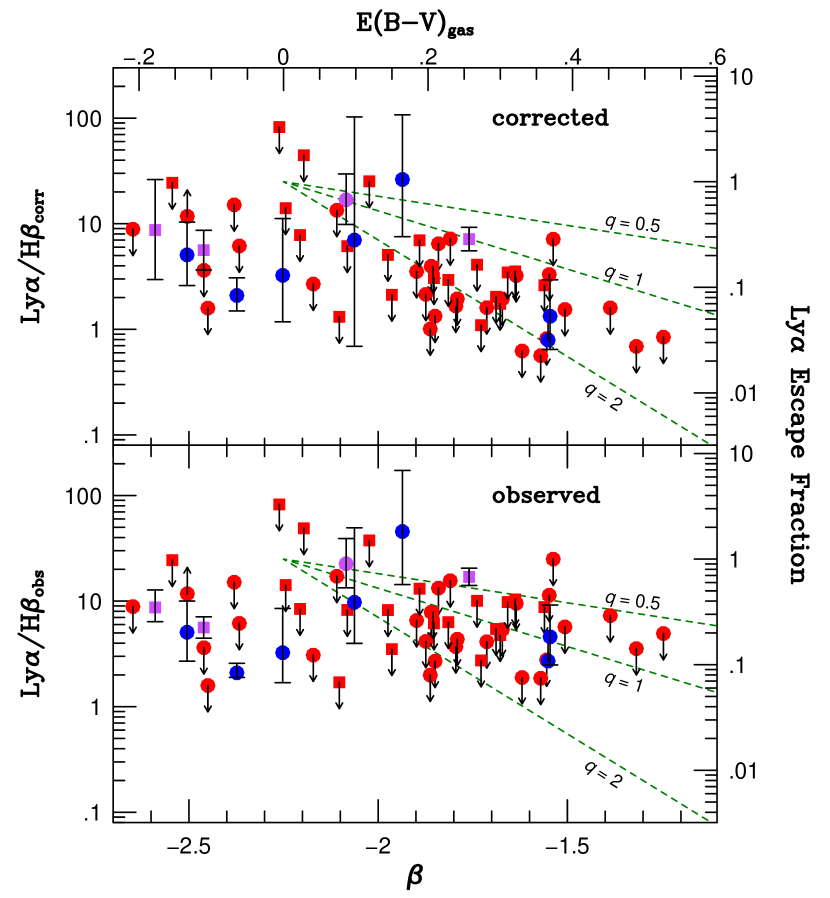
Figure 1.— Ly$\alpha$/H$\beta$ ratios for $1.92<z<2.35$ HST-grism galaxies plotted against the power-law slope of the galaxies’ rest-frame UV continua ($\beta$) and their corresponding nebular extinction [$E(B-V)$], assuming a Calzetti (2001) obscuration relation. The red points show Ly$\alpha$ upper limits from the integral-field spectroscopy of the HETDEX Pilot Survey, with the circles representing COSMOS field objects and the squares denoting sources in GOODS-N. The purple points indicate HPS objects with both Ly$\alpha$ and H$\beta$ detections. For comparison, the blue points are the ratios of GOODS-S LAEs detected via narrow-band imaging. The bottom panel presents the observed data, while the top panel corrects the H$\beta$ line fluxes for extinction using the slope of the UV continuum and the relation between stellar reddening and obscuration given by Calzetti (2001). (Objects with $\beta<-2.25$ have been assigned zero reddening.) The green dashed lines show where the optical depth to Ly$\alpha$ is 0.5, 1.0, and 2.0 times that of the continuum at 1216 Å. After correcting for extinction, most, if not all the galaxies lie below this line, demonstrating the importance of resonant Ly$\alpha$ scattering within these galaxies.

The top panel of Figure 1 repeats our Ly$\alpha$/H$\beta$ comparison, but with H$\beta$ corrected for extinction via the Calzetti (2001) obscuration relation and the assumption that $\beta_{0}=-2.25$. These values can easily be translated into escape fractions. Under Case B recombination, every ionization results in the creation of a Balmer-line photon, with $\sim 11.5\%$ of these photons coming via an $n=4$ to $n=2$ transision (i.e., H$\beta$; Pengelly, 1964; Osterbrock & Ferland, 2006). Three quarters of these Balmer transitions land in a $2P$ orbital and immediately decay to the ground state via the emission of Ly$\alpha$; the other 25% of the electrons become temporarily trapped in the $2S$ state before decaying to $n=1$ via two-photon emission. Thus, under normal conditions, the Ly$\alpha$/H$\beta$ ratio should be

$$R=\frac{I({\rm Ly}\alpha)}{I({\rm H}\beta)}=\frac{3}{4}\,\frac{\alpha_{B}}{\alpha_{{\rm H}\beta}^{\rm eff}}\,\frac{h\nu_{{\rm Ly}\alpha}}{h\nu_{{\rm H}\beta}}\approx 25$$ (3)

where $\alpha_{B}$ is the Case B recombination coefficient ($2.59\times 10^{-13}$ cm³ s^-1 at 10,000 K) and $\alpha_{{\rm H}\beta}^{\rm eff}$ is the effective Case B recombination coefficient for H$\beta$ ($3.03\times 10^{-14}$ cm³ s^-1 at $T=10000$ K; Pengelly, 1964; Osterbrock & Ferland, 2006).

The escape fractions shown in Figure 1 used $R=25$ as the intrinsic ratio of Ly$\alpha$ to H$\beta$. In practice, however, these escape fractions are upper limits. If the Case B condition is relaxed so that the Lyman continuum is optically thin, then the Ly$\alpha$/H$\beta$ ratio may be boosted to values as large as $R\sim 33$, thereby lowering $f_{\rm esc}^{{\rm Ly}\alpha}$. Most evidence suggests that at the redshifts considered here, the escape fraction of Lyman continuum photons is at most a couple of percent (e.g., Chen et al., 2007; Iwata et al., 2009; Vanzella et al., 2010), but this possibility cannot be excluded. Similarly, if the ISM density approaches $n_{e}/\sqrt{T_{e}/10^{4}}\gtrsim 10^{4}$ cm^-3 collisions will redistribute $2S$ electrons into the $2P$ state, again enhancing Ly$\alpha$ relative to H$\beta$. In the galaxies of the local universe, most H II regions have electron densities between 1 and 100 cm^-3 (e.g., Gutiérrez & Beckman, 2010), though this number may be slightly larger in dwarf systems (e.g., Hunter & Hoffman, 1999). Shocks or very high densities (such as in the broad-line regions of AGN) may also increase Ly$\alpha$ relative to H$\beta$ by creating an environment where the $n=2$ state of neutral material is collisionally populated. Finally, our estimates of nebular reddening assume that the observed $z\sim 2$ galaxies have been undergoing vigorous star formation for at least $\sim 0.5$ Gyr, so that $\beta_{0}=-2.25$. Since all our grism-selected objects have very high H$\beta$ equivalent widths, the intrinsic slopes of their rest-frame UV continua are unlikely to be flatter than this value (Zeimann et al., 2014). However, $\beta_{0}$ could be steeper, up to $-2.7$ in the extreme, if the systems have only recently begun their star forming activity (Calzetti, 2001). In this case, our reddening estimates would be underestimated, H$\beta$ would be enhanced, and, once again, our inferred ratios of Ly$\alpha$ to H$\beta$ would need to be reduced.

In summary, our adopted values of $R=25$ and $\beta_{0}=-2.25$ both produce upper limits for the Ly$\alpha$ escape fraction. Any deviations from simple Case B recombination or steady-state star formation will only serve to reduce $f_{\rm esc}^{{\rm Ly}\alpha}$. While factor of $\sim 2$ errors are theoretically possible for systems younger than $\sim 2$ Myr, in most cases, any systematic error associated with our escape fraction measurements should be less than $\sim 30\%$.

As the upper panel of Figure 1 illustrates, the median H$\beta$ emitter detected by the HST grism has an escape fraction below 7%, with no statistical difference between the results of the two HPS fields. Note that our constraints on $f_{\rm esc}^{{\rm Ly}\alpha}$  become progressively stronger as the slope of the UV continuum becomes redder. This is simply the result of our extinction law: as the stellar reddening increases, so does the assumed extinction correction for H$\beta$. The implied increase in H$\beta$ then translates into a decreased limit for the Ly$\alpha$/H$\beta$ ratio.

Another way to view the data of Figure 1 is through the mathematics of survival analysis (Cohen, 1991; Lee & Wang, 2003; Feigelson & Babu, 2012). Several authors have shown that the distribution of Ly$\alpha$ equivalent widths is exponential in form above a rest-frame equivalent width of $\sim 20$ Å (Gronwall et al., 2007; Nilsson et al., 2009; Ciardullo et al., 2012). If the same is true for Ly$\alpha$ escape fractions, then the computation of the median escape fraction is straightforward. The result is a most likely median value of $f_{\rm esc}^{{\rm Ly}\alpha}=5.9^{+1.0}_{-0.9}$%, where the errors are computed via a Markov Chain Monte Carlo sampler (Foreman-Mackey et al., 2013). Of course, since this calculation depends on the underlying shape of the distribution, the formal errors on $f_{\rm esc}^{{\rm Ly}\alpha}$  underestimate the true uncertainty in the measurement.

Perhaps the most instructive way to interpret Figure 1 is through the geometric parameter $q$, which has been defined by Finkelstein et al. (2008) as the ratio of the optical depth of Ly$\alpha$ to that of the stellar continuum at 1216 Å. In objects where resonant scattering is important and the escape path for Ly$\alpha$ photons is long, the likelihood of such a photon encountering a dust grain is large and $q>1$. Conversely, if $q\sim 1$, Ly$\alpha$ must have a relatively direct escape route from the galaxy, with a path-length similar to that of the star light. Values of $q<1$ point to either anisotropic emission, a spatial offset between the points of origin for Ly$\alpha$ and the continuum, a clumpy ISM (Neufeld, 1991; Hansen & Oh, 2006), or significant deviations from Case B recombination.

The dashed lines Figure 1 display the $q=0.5,1$ and 2 relations under the assumption that a Calzetti (2001) obscuration relation holds, with $A_{1216}=2.77\,\Delta\beta$. As expected, most of the sources have upper limits that are larger than $q=1$, demonstrating that resonant scattering of Ly$\alpha$ photons within these galaxies is significant. Perhaps as importantly, none of the objects show values of $q$ significantly less than one. Several studies have found that luminous Ly$\alpha$ emitting galaxies tend to cluster about the $q=1$ line (e.g., Finkelstein et al., 2009, 2011; Blanc et al., 2011; Nakajima et al., 2012), and Hagen et al. (2014a) found that small values of $q$ are common in compact, low-mass LAEs. But these analyses were for systems selected via their strong Ly$\alpha$ emission. The sources analyzed here were primarily chosen via their bright [O III] (or [O II]) lines. In these more normal star-forming galaxies, $q$ is generally greater than one, demonstrating that Ly$\alpha$ has a difficult time escaping its immediate environment.

4. The Global Escape Fraction

An alternative approach to exploring the escape fraction of Ly$\alpha$ photons from the $z\sim 2$ universe is to do so globally, via a comparison of the H$\beta$ and Ly$\alpha$ luminosity functions. The $\sim 100,000$ Mpc³ volume of space surveyed for both H$\beta$ and Ly$\alpha$ contains 67 galaxies detected in H$\beta$ and 23 identifiable via Ly$\alpha$. These numbers are more than sufficient for defining the emission-line luminosity functions of the two galaxy populations and integrating for their total luminosity density.

4.1. The H$\beta$ Luminosity Function

In order to calculate the $z\sim 2$ H$\beta$ luminosity function, we must first estimate the effective area of overlap between the HPS and the HST grism observations. This is not just a simple geometry problem, since, as with all slitless spectroscopy, overlapping sources render a fraction of the survey area unusable. Zeimann et al. (2014) estimated this fraction via a series of Monte Carlo experiments, in which realistic magnitude and positional distributions were used to create simulated frames, which were then “observed” in the same manner as the original data. At each point on the simulated frames, the amount of contamination was compared to the local sky noise, and all regions where the systematics of spectral subtraction were greater than this noise were excluded from consideration. Since sky noise is the dominant source of uncertainty for all $z\sim 2$ observations, this procedure generated a reliable statistical measure of the grism survey’s effective area. Based on the results of these simulations, we reduced the geometric HPS/HST overlap region by 15% to 65 arcmin², and used this new area in our calculation of survey volume.

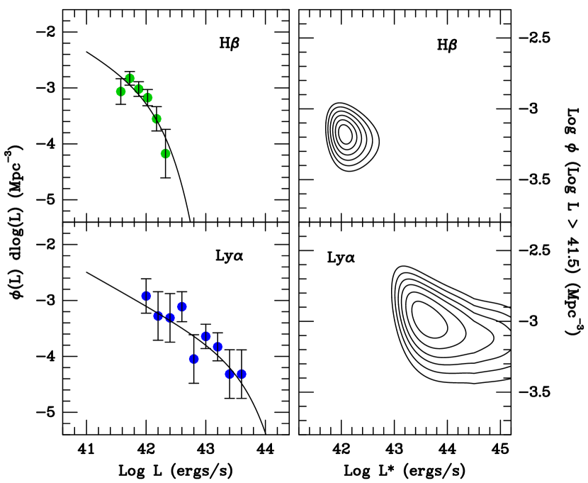
Figure 2.— The H$\beta$ and Ly$\alpha$ luminosity functions in the $1.92<z<2.35$ regions surveyed for both emission lines. The left-hand panels show the observed luminosity functions (binned into 0.15 dex and 0.20 dex intervals for H$\beta$ and Ly$\alpha$, respectively), and the best-fit Schechter (1976) functions. The right panels display the likelihood contours (in $0.5\,\sigma$ intervals) of the fitted functions, with $\log L^{*}$ on the $x$-axis and the number density of galaxies brighter than $\log L=41.5$ (ergs s^-1) on the $y$-axis. The slope of the faint end of the luminosity function has been fixed at $\alpha=-1.6$.

To measure the total H$\beta$ luminosity density at $z\sim 2$, we began by following the procedures described by Blanc et al. (2011) and applied the $1/V_{\rm max}$ technique (Schmidt, 1968; Huchra & Sargent, 1973) to the H$\beta$ sources found in COSMOS, GOODS-N, and GOODS-S. As described in Zeimann et al. (2014), the completeness fraction of our HST grism sample, as a function of H$\beta$ flux, has been calculated via a series of Monte Carlo simulations; in summary, the 50% completeness limit for the two GOODS fields (in ergs cm^-2 s^-1) occurs at $\log F_{{\rm H}\beta}=-17.06$, while for COSMOS, this limit is $\log F_{{\rm H}\beta}=-16.88$. In the regions of overlap between the H$\beta$ and Ly$\alpha$ surveys, 42 galaxies are present above these completeness limits. Using these data, we computed $V_{\rm max}$, the co-moving volume over which an object with H$\beta$ luminosity $L$ would be detected more than 50% of the time. The number density of galaxies in any absolute luminosity bin of width $\Delta\log L$ is then

$$\phi(\log L)=\frac{1}{\Delta(\log L)}\,\eta\,\sum_{i}\left\{\frac{1}{V_{\rm max}(i)}\right\}$$ (4)

where $\eta$ is the inverse of the completeness function, and the summation is performed over all galaxies with luminosities falling within the bin. The top-left panel of Figure 2 displays this function, where the uncertainties on the points are from Poissonian statistics only.

We next fit this function using the maximum-likelihood procedure detailed in Ciardullo et al. (2013). We began with the assumption that over the redshift range $1.92<z<2.35$, the H$\beta$ luminosity function can be modeled via a Schechter (1976) law

$$\phi(L/L^{*})d(L/L^{*})=\phi^{*}\left(L/L^{*}\right)^{\alpha}e^{-L/L^{*}}d(L/L^{*})$$ (5)

with $L^{*}$ being the characteristic monochromatic luminosity of the epoch. The observed function, of course, does not follow this relation, as incompleteness takes an ever increasing toll at fainter fluxes. Hence we define $\phi^{\prime}(L,z)$ as the Schechter function modified by the flux-dependent completeness fraction at each redshift as given by Zeimann et al. (2014). From Poissonian statistics, the probability of observing $n$ galaxies in any given luminosity and volume interval $\Delta L\,\Delta V$ is then

$$p(n|\lambda)=\frac{\lambda^{n}e^{-\lambda}}{n!}$$ (6)

where the expectation value $\lambda=\phi^{\prime}(L,z)\Delta L\,\Delta V$. If we let these intervals become differentials, then the likelihood of drawing an observed set of $N$ H$\beta$ luminosities from a given Schechter function with parameters $L^{*}$, $\phi^{*}$, and $\alpha$ becomes

$$\ln P=-\int_{z_{1}}^{z_{2}}\int_{L_{\rm min}(z)}^{\infty}\phi^{\prime}(L,z)dL\,dV+\sum_{i}^{N}\ln\phi^{\prime}(L_{i},z_{i})$$ (7)

where, for purposes of our analysis, we define the lower limits of the luminosity integral by where the completeness fraction drops to 50%. The top right panel of Figure 2 displays the likelihood contours in $L^{*}$ and $\phi^{*}$, with the faint-end slope fixed at $\alpha=-1.6$ for consistency with other studies (Hayes et al., 2010; Ly et al., 2011; Sobral et al., 2013). To avoid the well-known degeneracy between $L^{*}$ and $\phi^{*}$, the ordinate of the plot gives the integral of the Schechter function (down to $\log L=41.5$ ergs s^-1), rather than the traditional coefficient, $\phi^{*}$. The most likely solution, with $\log L^{*}=42.07$ and $\phi_{\rm tot}(\log L>41.5)=-3.18$ Mpc^-3, is displayed in the top left of Figure 2. For comparison, the most likely H$\beta$ luminosity function for the full sample of $1.90<z<2.35$ HST-grism selected galaxies in COSMOS, GOODS-N, and GOODS-S has $\log L=42.07$ and $\phi_{\rm tot}(\log L>41.5)=-3.28$.

Table 2 lists the most-likely Schechter (1976) function parameters, their uncertainties, and the total integrated H$\beta$ luminosity density

$$\rho_{{\rm H}\beta}=\phi^{*}L^{*}\,\Gamma(\alpha+2)$$ (8)

for the $1.92<z<2.35$ regions of overlap between the HST surveys, HPS, and the CDF-S narrow-band survey field. Although this latter quantity does require the extrapolation of the Schechter (1976) function to zero luminosity, this extension is not an important issue, as galaxies below our detection threshold are predicted to contribute only $\sim 20\%$ to the universe’s total H$\beta$ luminosity density. For reference, Table 2 also lists the H$\beta$ luminosity function parameters for the entire $1.90<z<2.35$ grism survey region of COSMOS and GOODS. Although this full volume is roughly four times larger than that for the just the regions of survey overlap, the luminosity function defined by its galaxies is virtually identical to that of the smaller region.

The likelihoods given in Table 2 and displayed in Figure 2 represent only the formal statistical error of our fit. Not included are systematic uncertainties associated with the data themselves, most notably, with the completeness corrections. Our estimates for the survey area and completeness fraction are based on the simulations performed by Zeimann et al. (2014), who also confirmed that metallicity, equivalent width, and redshift are not important factors for determining the detectability of H$\beta$. This analysis did not, however, take galaxy size into account, and this can be an important factor for slitless spectroscopic surveys. Fortunately, for the dataset considered here, the effect is minor. As van der Wel et al. (2014) have shown, $\sim 84\%$ of massive ($M_{*}\gtrsim 10^{10}M_{\odot}$) late-type galaxies at $z=2.25$ have effective radii smaller than $0\farcs 45$, while all the H$\beta$ galaxies analyzed here have $r_{e}<0\farcs 50$ (Hagen et al., 2014b). In this regime, the completeness of an HST grism survey is a very weak function of size (see the analysis of Colbert et al., 2013), and the simulations of Zeimann et al. (2014) should be valid. Based on this result, our calculation of survey area and incompleteness fraction likely carries an additional error of $\sim 8\%$.

Similarly, because the HST survey fields are relatively small, the effects of cosmic variance on our luminosity functions are non-negligible. We can estimate this number using the cosmic variance calculator developed by Trenti & Stiavelli (2008), which combines Press-Schechter theory with N-body cosmological simulations to predict field-to-field fluctuations in arbitrary slices (or pencil beams) of the universe. According to this estimator, our number counts in the three HST fields carry an additional uncertainty of $\sim 12\%$, while that for just the 65 arcmin² region of overlap between the HST-grism surveys and our two sets of ground-based Ly$\alpha$ observations is $\sim 20\%$. Of course, for estimates of the Ly$\alpha$ escape fraction, it is the field-to-field variations of galactic properties such as star formation rate and dust content which are the important parameters for the calculation, not simply the number of galaxies present in the region. While we are less able to quantify this number, it seems likely that the effect is significantly less than $\sim 20\%$.

The last piece of information needed to compute the H$\beta$ luminosity density of the $z\sim 2$ universe is an estimate of H$\beta$ attenuation. Once again, we are limited by the lack of direct knowledge of the galaxies’ nebular extinction. Measurements of the Balmer decrement in the $z\sim 2$ universe are rare, especially for samples of emission-line selected galaxies. (The closest comparison sample to our own – that created by Domínguez et al. (2013) from 128 WFC3 grism-selected galaxies in the $0.75<z<1.5$ universe — has very large uncertainties, with a mean value of $c_{{\rm H}\beta}\sim 1.0\pm 1.0$ dex.) Consequently, we must again compute the loss of H$\beta$ statistically from measurements of the stellar continuum. We did this by translating the UV slopes of each H$\beta$ source in our sample into a nebular extinction using the obscuration relations of Calzetti (2001), and then examining the distribution of these extinctions. If we just consider the sample of 42 galaxies in the region of space surveyed for H$\beta$ and Ly$\alpha$, then the median logarithmic extinction at H$\beta$ is $c_{{\rm H}\beta}=0.35$, while the effective extinction, defined via the total amount of H$\beta$ luminosity lost due to dust in all the galaxies, is $c_{{\rm H}\beta}=0.44$. For comparison, the logarithmic extinctions found for all $1.90<z<2.35$ galaxies brighter than the 50% H$\beta$ completeness limit in the HST fields of COSMOS, GOODS-N, and GOODS-S is $c_{{\rm H}\beta}=0.31$ (median) and $c_{{\rm H}\beta}=0.59$ (effective). This difference between the median and effective attenuation is not unexpected: as noted by many authors, reddening is strongly correlated with stellar mass and therefore star-formation rate (e.g., Moustakas et al., 2006; Garn & Best, 2010; An et al., 2014). Since the brightest H$\beta$ emitters are also those most heavily extinguished by dust, the effective extinction of the sample should be larger than the median extinction. For the remainder of this paper, we will adopt $c_{{\rm H}\beta}=0.5$ as the total logarithmic extinction at H$\beta$, while noting that the uncertainty on this number is likely to be $\pm 0.1$ dex. The resulting intrinsic H$\beta$ luminosity density and total error for the $z\sim 2$ universe is then $\log\rho_{{\rm H}\beta}=39.49\pm 0.12$ (ergs s^-1 Mpc^-3).

Our H$\beta$ luminosity function is the first such measurement at $z\gtrsim 2$. However, there have been previous estimates of the epoch’s H$\alpha$ luminosity function from deep, narrow-band surveys in the infrared. While Hayes et al. (2010) found $\log L^{*}({\rm H}\alpha)=43.22$ (ergs s^-1) and a total H$\alpha$ luminosity density of $\log\rho_{{\rm H}\alpha}=39.77$ (ergs s^-1 Mpc^-3) in a 56 arcmin² region of GOODS-S, a much larger ($\sim 2$ deg²) study by Sobral et al. (2013) inferred $\log L^{*}({\rm H}\alpha)=42.47$ and $\log\rho_{{\rm H}\alpha}=40.01$. Our best-fit H$\beta$ function, coupled with an effective logarithmic extinction of $c_{{\rm H}\beta}=0.5$, a Cardelli et al. (1989) extinction law (with $R_{V}=3.1$) and an assumed intrinsic H$\alpha$/H$\beta$ ratio of 2.86 (Pengelly, 1964; Osterbrock & Ferland, 2006) implies observed values for $L^{*}$ and the H$\alpha$ luminosity density of $\log L({\rm H}\alpha)=42.68$ (ergs s^-1) and $\log\rho_{{\rm H}\alpha}=39.70$ (ergs s^-1 Mpc^-3). In other words, our measurement of $L^{*}$ is in good agreement with that of Sobral et al. (2013), but our estimated luminosity density is more in line with that found by Hayes et al. (2010). It is somewhat surprising that these three surveys differ by more than 0.3 dex in their determination of luminosity density, but given the small volumes involved (5440, 77,000, and 108,000 Mpc³ for the Hayes et al. (2010), Sobral et al. (2013), and this survey, respectively), and the expected cosmic variance in the number counts ($\sim 50\%,15\%$, and 20%; Trenti & Stiavelli, 2008), the result is still reasonable.

We can also test our measurement of the H$\beta$ luminosity function by converting it into a star formation rate. The observed H$\beta$ luminosity density in our HST fields is $\log\rho_{{\rm H}\beta}=38.99\pm 0.04$ (ergs s^-1 Mpc^-3). If we again de-redden this number by $c_{{\rm H}\beta}=0.5$ and assume an intrinsic H$\alpha$/H$\beta$ ratio of 2.86, then $\log\rho_{{\rm H}\alpha}=39.95$ (ergs s^-1 Mpc^-3). The application of the local H$\alpha$ star-formation rate calibration (Hao et al., 2011; Murphy et al., 2011; Kennicutt & Evans, 2012) then yields $\log\rho_{\rm SFR}\sim-1.3\pm 0.1$ ($M_{\odot}$ yr^-1 Mpc^-3) where the error is dominated by the uncertainty in the reddening correction. This value is generally consistent with most other determinations of the epoch’s star-formation rate density (e.g., Hopkins, 2004; Wilkins et al., 2008; Bouwens et al., 2010), although, as pointed out above, it is slightly lower than that found from the H$\alpha$ observations of Sobral et al. (2013).

4.2. The Ly$\alpha$ Luminosity Function and $f_{\rm esc}^{{\rm Ly}\alpha}$

To compute the volumetric Ly$\alpha$ escape fraction of the $z\sim 2$ universe, we repeated the above analysis using the Ly$\alpha$ emitting galaxies found in our overlapping survey area. For the HPS objects, this involved using the estimates of completeness versus line flux computed by Adams et al. (2011) for the 186 separate VIRUS-P pointings covering the HST-grism fields in COSMOS and GOODS-N; for the narrow-band data, the completeness fraction versus monochromatic flux relation was based on the artificial star experiments performed by Ciardullo et al. (2012) on the region’s deep Mosaic images. These functions were then folded into the $1/V_{\rm max}$ calculation of equation (4) and the luminosity function was fit using the maximum-likelihood procedures described by equation (7).

Figure 3.— Our maximum likelihood solution for the escape fraction of Ly$\alpha$ photons from our $\sim 100,000$ Mpc³ survey regions at $1.92<z<2.35$. The plot assumes steady-state star formation for at least $\sim 0.5$ Gyr, an effective logarithmic H$\beta$ extinction of $c_{{\rm H}\beta}=0.5$, that $\sim 20\%$ of Ly$\alpha$ photons arise from low equivalent width objects, and that Case B recombination holds. Errors in the latter two assumptions would likely drive the escape fraction to lower values.

The results are shown in the bottom panels of Figure 2 and summarized in Table 2. Because our survey fields contain far fewer LAEs than H$\beta$ galaxies, the Ly$\alpha$ luminosity function is not as well defined as its H$\beta$ counterpart. Indeed, only 11 HPS galaxies and 6 narrow-band selected objects have Ly$\alpha$ detections that are brighter than their frame’s 50% completeness limit. As a result, the “knee” of the Schechter (1976) function is poorly defined and detected only with $\sim 2\,\sigma$ significance. Nevertheless, the best fit function, with $\log L=43.60$ (ergs s^-1) and $\log\phi^{*}=-4.45$ (Mpc^-3), is similar to that found by Blanc et al. (2011) for the entire sample of 49 non-X-ray-emitting HPS LAEs with $1.9<z<2.8$. Our $z\sim 2$ value of $\log L^{*}$ is significantly larger that those found by narrow-band surveys (Ciardullo et al., 2012; Gronwall et al., 2014), but, given the vastly larger volume studied by the HPS and the increased likelihood of finding rare, exceptionally bright objects, this difference is not a serious concern.

Despite the rather large uncertainty associated with $\log L^{*}$, the total Ly$\alpha$ luminosity density of the $z\sim 2$ universe, as defined through equation (8), is very well defined, with $\log\rho_{{\rm Ly}\alpha}=39.56\pm 0.11$ (ergs s^-1 Mpc^-3). This number is a slight underestimate, since, unlike the HST grism, the HPS and the narrow-band surveys do not unambiguously identify every Ly$\alpha$ source above a flux limit. To be classified as an LAE, a galaxy must also have a rest-frame equivalent width greater than 20 Å. (Lower equivalent width objects can be confused with foreground sources and are usually ignored.) To correct for these missing objects, one must estimate the total amount of emission associated with low-equivalent width galaxies. If the equivalent width distribution of such objects follows the exponential function defined by the higher EW LAEs, then our census may be missing between 20% and 30% of escaping Ly$\alpha$ photons (Ciardullo et al., 2012; Gronwall et al., 2014). Alternatively, if, as suggested by Shimasaku et al. (2006), the true distribution of Ly$\alpha$ equivalent widths has a lognormal form similar to that associated with local [O II] emitting galaxies (e.g., Blanton & Lin, 2000), then the missing Ly$\alpha$ flux would be far less. Since observations of Lyman-break galaxies appear to support the former possibility (e.g., Shapley et al., 2003; Kornei et al., 2010), we use this more conservative approach in our calculations and assume that we are missing $\sim 20\%$ of the epoch’s total Ly$\alpha$ luminosity density.

Figure 3 combines our two likelihood functions to show the total Ly$\alpha$ escape fraction within our $\sim 100,000$ Mpc³ survey volume. In the figure, the most probable escape fraction for the $z\sim 2$ universe is $4.4^{+2.1}_{-1.2}\%$, with the bulk of our statistical error arising from the uncertainty in the Ly$\alpha$ luminosity function. We must note, however, that the systematic errors associated with our measurement may be greater than this. While our assumptions about Case B recombination, the history of $z\sim 2$ star formation, and the population of low equivalent width Ly$\alpha$ emitters suggest that our measurement of $f_{\rm esc}^{{\rm Ly}\alpha}$  is an upper limit, the greatest uncertainty is that associated with internal extinction. As mentioned above, none of the objects studied in this program have measured Balmer decrements; instead, we have estimates of the stellar reddenings derived from the observed slopes of the rest-frame UV continua. These are, at best, indirectly related to the nebular extinctions applicable to our problem (Calzetti, 2001). To produce Figure 3, we have assumed $c_{{\rm H}\beta}=0.5$, but this number likely has an uncertainty of $\pm 0.1$ dex. This factor adds an additional $\sim 25\%$ error onto our estimate, making our systematic error term comparable to our statistical uncertainty.

5. Discussion and Conclusions

Our estimate of $4.4^{+2.1}_{-1.2}\%$ for the Ly$\alpha$ escape fraction is consistent with the study by Blanc et al. (2011), who normalized their $1.9<z<2.8$ LAE observations via rest-frame UV measurements of the epoch’s star formation rate density. It also agrees with most models for the evolution of $f_{\rm esc}^{{\rm Ly}\alpha}$ with redshift (Hayes et al., 2011; Blanc et al., 2011; Dijkstra & Jeeson-Daniel, 2013). But these analyses rely predominantly on indirect measurements: in fact, the only previous study to directly compare Ly$\alpha$ emission with Ly$\alpha$ production is that of Hayes et al. (2010). By performing dual narrow-band surveys in Ly$\alpha$ and H$\alpha$, and estimating nebular extinction via the reddening of the stellar rest-frame UV continuum, Hayes et al. (2010) obtained $5.3\pm 3.8$% as the Ly$\alpha$ escape fraction for the $z=2.2$ universe. Our $1.92<z<2.35$ measurements, which also rely on stellar reddenings, encompass a volume $\sim 20$ times larger than that of the Hayes et al. (2010) survey, and are therefore far less sensitive to issues associated with cosmic variance. More importantly, by surveying this larger volume, we have been able to better define the bright end of the Ly$\alpha$ and H$\beta$ luminosity functions. While our data are not as good as those of Hayes et al. (2010) for defining the slope of the faint-end of the luminosity function (we adopt $\alpha=-1.6$, rather than fitting for the variable), we have many more $L>L^{*}$ galaxies, and, unless the Schechter (1976) function has a very steep, faint-end slope, it is this latter parameter which is most important for defining the total emission-line flux. Of course, our observations also have the drawback of being based on H$\beta$, rather than H$\alpha$, and are thus more sensitive to the effects of dust and internal extinction than the previous study.

At present, our measurements of $f_{\rm esc}^{{\rm Ly}\alpha}$ are limited by two factors: the depth of our survey for Ly$\alpha$, and our ability to estimate $c_{{\rm H}\beta}$ for individual galaxies. Both of these issues should improve rather rapidly.

At the wavelengths considered here, the HPS typically reached a monochromatic flux limit of $\sim 1.5\times 10^{-16}$ ergs cm^-2 s^-1, or $\log L({{\rm Ly}\alpha})\sim 42.7$ (ergs s^-1) at $z\sim 2.2$. Unfortunately, as shown in Figure 1, this is not deep enough to detect many of the emission-line galaxies found by the HST grism, as our median upper limit on the Ly$\alpha$ escape fraction is $\sim 6\%$. In other words, our detection threshold lies just above that expected from our analysis of the epoch’s volumetric escape fraction. The main HETDEX survey, which begins in 2015, is designed to reach Ly$\alpha$ flux limits that are a factor of $\sim 3$ fainter than that for the HPS, i.e., $\sim 0.5\times 10^{-16}$ ergs cm^-2 s^-1 at $\sim 3900$ Å. This limit should allow us to directly measure $f_{\rm esc}^{{\rm Ly}\alpha}$ for the typical star-forming galaxy of the epoch, and enable a search for trends with object size, stellar mass, and star formation rate.

Similarly, our ability to measure the intrinsic Balmer line luminosities of the H$\beta$-selected galaxies is rapidly advancing. Like most previous studies of Ly$\alpha$ emission at $2<z<3$ (e.g., Gronwall et al., 2007; Hayes et al., 2010; Blanc et al., 2011), our estimates of nebular extinction are inferred from measurements of stellar reddening, and, while there may be a relation between the two parameters, this unknown does introduce an uncertainty into the calculation. Fortunately, instruments are now available which allow simultaneous infrared spectroscopy for large numbers of $z\sim 2$ sources (e.g., Eikenberry et al., 2012; McLean et al., 2012), thereby enabling direct measurements of the galaxies’ Balmer decrements. This capability will remove the most important source of systematic error from the analysis.

Table 1H$\beta$ and Ly$\alpha$ Galaxy Measurements

				$\log$ Flux (ergs cm-2 s-1)
$\alpha(2000)$	$\delta(2000)$	$z$	$\beta$	H$\beta$	Ly$\alpha$
COSMOS
10:00:35.54	$+$02:13:03.0	1.934	$-1.25\pm 0.06$	$-16.57\pm 0.11$	$<-15.88$
10:00:36.67	$+$02:13:07.7	2.092	$-1.55\pm 0.12$	$-17.18\pm 0.45$	$<-16.12$
10:00:33.96	+02:13:16.0	2.230	$-2.30\pm 0.05$	…	$-15.55_{-0.07}^{+0.12}$
10:00:17.30	$+$02:19:26.5	2.084	$-1.54\pm 0.06$	$-17.27\pm 0.36$	$<-15.87$
10:00:15.73	$+$02:20:28.1	1.975	$-1.64\pm 0.15$	$-16.78\pm 0.08$	$<-15.81$
10:00:47.16	$+$02:17:44.5	2.025	$-1.62\pm 0.02$	$-16.09\pm 0.03$	$<-15.82$
10:00:41.65	$+$02:18:00.2	2.095	$-1.39\pm 0.03$	$-16.84\pm 0.16$	$<-15.98$
10:00:40.82	$+$02:18:22.9	2.070	$-1.63\pm 0.01$	…	$-15.59_{-0.17}^{+0.21}$
10:00:42.91	$+$02:18:25.6	2.096	$-1.90\pm 0.04$	$-16.73\pm 0.09$	$<-15.91$
10:00:38.64	$+$02:18:36.3	1.927	$-1.79\pm 0.08$	$-16.36\pm 0.08$	$<-15.79$
10:00:42.21	$+$02:18:48.5	2.290	$-1.85\pm 0.08$	$-16.59\pm 0.07$	$<-16.16$
10:00:18.68	$+$02:14:59.9	2.310	$-0.33\pm 0.70$	…	$-15.41_{-0.10}^{+0.13}$
10:00:21.92	$+$02:15:40.0	2.093	$-2.46\pm 0.11$	$-16.71\pm 0.08$	$<-16.15$
10:00:20.69	$+$02:12:53.4	2.163	$-1.55\pm 0.11$	$-16.65\pm 0.08$	$<-16.21$
10:00:23.79	$+$02:13:10.4	2.107	$-2.50\pm 0.24$	$<-17.06$	$-15.99_{-0.17}^{+0.22}$
10:00:17.22	$+$02:13:38.0	2.105	$-1.67\pm 0.09$	$-16.89\pm 0.14$	$<-16.16$
10:00:19.19	$+$02:14:06.6	2.103	$-1.86\pm 0.05$	$-16.61\pm 0.09$	$<-16.31$
10:00:23.61	$+$02:15:57.4	2.088	$-1.57\pm 0.05$	$-16.43\pm 0.06$	$<-16.17$
10:00:29.58	$+$02:17:02.8	1.921	$-1.86\pm 0.03$	$-16.35\pm 0.05$	$<-15.45$
10:00:28.64	$+$02:17:48.7	2.093	$-2.49\pm 0.04$	…	$-14.84_{-0.03}^{+0.07}$
10:00:27.24	$+$02:17:31.6	2.283	$-2.08\pm 0.07$	$-16.70\pm 0.20$	$-15.35_{-0.11}^{+0.13}$
10:00:22.88	$+$02:17:14.0	2.220	$-1.71\pm 0.10$	$-16.82\pm 0.11$	$<-16.21$
10:00:26.61	$+$02:17:14.5	2.224	$-2.65\pm 0.12$	$-17.13\pm 0.22$	$<-16.18$
10:00:24.22	$+$02:14:11.7	2.104	$-1.32\pm 0.05$	$-16.81\pm 0.14$	$<-16.26$
10:00:25.45	$+$02:14:27.8	2.166	$-2.17\pm 0.16$	$-16.67\pm 0.09$	$<-16.18$
10:00:23.41	$+$02:14:32.3	2.097	$-1.79\pm 0.14$	$-16.74\pm 0.08$	$<-16.10$
10:00:23.23	$+$02:12:30.7	2.225	$-2.45\pm 0.11$	$-16.40\pm 0.08$	$<-16.20$
10:00:39.12	$+$02:14:51.0	2.125	$-1.51\pm 0.04$	$-16.49\pm 0.06$	$<-15.73$
10:00:32.33	$+$02:14:53.0	1.975	$-2.37\pm 0.06$	$-16.37\pm 0.05$	$<-15.58$
10:00:32.60	$+$02:15:35.9	2.162	$-1.87\pm 0.05$	$-16.45\pm 0.06$	$<-15.83$
10:00:34.08	$+$02:15:54.4	2.199	$-1.81\pm 0.13$	$-16.99\pm 0.17$	$<-15.79$
10:00:44.93	$+$02:15:53.2	2.093	$-2.38\pm 0.13$	$-16.84\pm 0.08$	$<-15.67$
10:00:37.02	$+$02:17:47.5	1.940	$-2.11\pm 0.14$	$-16.96\pm 0.11$	$<-15.72$
10:00:29.81	$+$02:18:49.2	2.200	$-1.69\pm 0.05$	…	$-15.38_{-0.06}^{+0.06}$
10:00:19.55	$+$02:17:56.1	2.052	$-1.84\pm 0.07$	$-16.97\pm 0.31$	$<-15.85$
GOODS-N
12:36:15.00	$+$62:13:29.9	1.998	$-1.97\pm 0.20$	$-16.66\pm 0.06$	$<-15.72$
12:36:20.46	$+$62:14:52.2	1.999	$-2.26\pm 0.38$	$-17.21\pm 0.15$	$<-15.29$
12:36:15.86	$+$62:13:25.7	2.086	$-2.20\pm 0.30$	$-17.58\pm 0.37$	$<-15.90$
12:36:18.78	$+$62:10:37.3	2.264	$-1.73\pm 0.12$	$-16.55\pm 0.06$	$<-16.11$
12:36:20.07	$+$62:11:12.4	2.004	$-1.64\pm 0.11$	$-16.76\pm 0.09$	$<-15.75$
12:36:13.33	$+$62:11:45.2	2.258	$-1.74\pm 0.25$	$-16.93\pm 0.11$	$<-15.93$
12:36:24.96	$+$62:12:23.6	2.216	$-1.56\pm 0.18$	$-17.04\pm 0.16$	$<-16.10$
12:36:40.61	$+$62:13:10.9	2.051	$-1.81\pm 0.25$	$-16.89\pm 0.13$	$<-16.09$
12:36:35.42	$+$62:14:37.6	2.006	$-1.68\pm 0.06$	$-16.75\pm 0.41$	$<-16.07$
12:36:42.09	$+$62:13:31.4	2.018	$+0.52\pm 0.51$	$-17.25\pm 0.27$	$<-16.05$
12:36:44.90	$+$62:13:35.6	2.234	$-1.85\pm 0.43$	$-17.14\pm 0.12$	$<-16.35$
12:36:50.10	$+$62:14:01.2	2.235	$-1.49\pm 0.10$	…	$-15.61_{-0.06}^{+0.09}$
12:36:44.12	$+$62:14:01.9	2.273	$-0.12\pm 1.25$	…	$-15.69_{-0.21}^{+0.16}$
12:36:47.46	$+$62:15:03.5	2.083	$-2.46\pm 0.21$	$-16.69\pm 0.06$	$-15.94_{-0.08}^{+0.08}$
12:36:53.79	$+$62:15:21.7	2.022	$-2.54\pm 0.26$	$-17.22\pm 0.24$	$<-15.83$
12:36:55.60	$+$62:14:50.7	1.975	$-1.85\pm 0.21$	$-17.11\pm 0.13$	$<-16.21$
12:36:41.26	$+$62:11:15.6	2.062	$-1.96\pm 0.12$	$-16.38\pm 0.05$	$<-15.84$
12:36:55.06	$+$62:13:47.1	2.233	$-2.10\pm 0.10$	$-16.57\pm 0.05$	$<-16.33$
12:36:54.19	$+$62:13:35.9	2.263	$-2.59\pm 0.59$	$-16.86\pm 0.08$	$-15.92_{-0.11}^{+0.15}$
12:37:04.33	$+$62:14:46.2	2.220	$-1.76\pm 0.10$	$-16.33\pm 0.07$	$-15.11_{-0.04}^{+0.05}$
12:37:11.78	$+$62:13:38.9	1.914	$-2.08\pm 0.17$	$-16.71\pm 0.06$	$<-15.79$
12:37:11.20	$+$62:14:31.5	2.191	$-2.24\pm 0.24$	$-17.42\pm 0.27$	$<-16.27$
12:37:02.01	$+$62:14:19.1	2.291	$-2.21\pm 0.53$	$-17.09\pm 0.11$	$<-16.16$
12:36:53.32	$+$62:10:35.9	1.975	$-1.69\pm 0.09$	$-16.78\pm 0.11$	$<-16.04$
12:37:02.72	$+$62:10:10.8	1.989	$-1.66\pm 0.16$	$-16.51\pm 0.04$	$<-15.52$
12:37:11.00	$+$62:11:40.1	2.270	$-2.10\pm 0.15$	…	$-15.86_{-0.28}^{+0.20}$
12:37:07.10	$+$62:11:52.6	2.275	$-1.89\pm 0.11$	$-17.22\pm 0.20$	$<-16.10$
12:37:10.42	$+$62:10:35.5	2.161	$-2.02\pm 0.58$	$-17.43\pm 0.32$	$<-15.85$
GOODS-S
3:33:00.61	$-$27:40:27.0	2.030	$-1.55\pm 2.73$	$<-17.12$	$-16.69_{-0.09}^{+0.09}$
3:32:40.52	$-$27:49:32.5	2.042	$-2.06\pm 1.22$	$-17.06\pm 0.20$	$-16.49_{-0.09}^{+0.09}$
3:32:34.44	$-$27:47:42.8	2.030	$-2.00\pm 0.13$	$-16.73\pm 0.05$	…
3:32:41.55	$-$27:48:24.4	2.080	$-2.25\pm 0.44$	$-16.88\pm 0.25$	$-16.50_{-0.07}^{+0.07}$
3:32:42.19	$-$27:48:59.6	2.079	$-1.94\pm 0.26$	$-17.54\pm 0.49$	$-15.99_{-0.02}^{+0.02}$
3:32:28.85	$-$27:52:20.1	2.039	$-1.47\pm 0.18$	$-16.41\pm 0.05$	…
3:32:13.76	$-$27:43:00.5	2.070	$-2.50\pm 0.13$	$-16.83\pm 0.27$	$-16.13_{-0.03}^{+0.03}$
3:32:45.54	$-$27:53:43.3	2.059	$-1.55\pm 0.22$	$-17.17\pm 0.26$	$-16.53_{-0.08}^{+0.08}$
3:32:26.83	$-$27:46:01.8	2.079	$-1.15\pm 0.15$	$-16.75\pm 0.07$	…
3:32:25.82	$-27$:46:09.3	2.076	$-1.56\pm 0.30$	$-17.02\pm 0.13$	…
3:32:11.45	$-$27:50:26.7	2.068	$-2.37\pm 0.18$	$-16.29\pm 0.04$	$-15.97_{-0.02}^{+0.02}$
3:32:18.12	$-$27:49:41.9	2.034	$-1.77\pm 0.08$	$-16.90\pm 0.19$	…
3:32:59.11	$-$27:53:20.7	2.030	$-0.03\pm 0.09$	$-16.55\pm 0.18$	$-16.02_{-0.02}^{+0.02}$
3:32:04.00	$-$27:43:51.6	2.044	$-2.02\pm 0.58$	…	$-16.65_{-0.10}^{+0.10}$
3:32:08.66	$-$27:42:50.2	2.075	$-1.85\pm 0.12$	$-16.66\pm 0.16$	…
3:32:07.84	$-$27:42:27.2	2.049	$-1.22\pm 0.44$	$-16.61\pm 0.06$	…
3:32:09.60	$-$27:47:39.9	2.040	$-1.53\pm 0.21$	$-17.04\pm 0.12$	…
3:32:21.40	$-$27:51:26.2	2.037	$-1.14\pm 0.20$	$-16.52\pm 0.08$	…
3:32:46.15	$-$27:49:22.6	2.032	$-2.08\pm 0.10$	$-17.01\pm 0.14$	…
3:32:43.46	$-$27:43:36.5	2.078	$-0.51\pm 0.23$	$-16.90\pm 0.13$	…
3:32:23.24	$-$27:42:31.6	2.078	$-1.66\pm 0.16$	$-16.64\pm 0.04$	…
3:32:35.73	$-$27:46:39.0	2.073	$-0.50\pm 0.60$	$-16.99\pm 0.07$	…
3:32:35.60	$-$27:47:45.4	2.030	$-1.48\pm 0.49$	$-17.20\pm 0.10$	…
3:32:40.19	$-$27:46:54.6	2.069	$-0.64\pm 0.92$	$-17.35\pm 0.14$	$-16.36_{-0.05}^{+0.05}$

Table 2Best-Fit Schechter Function Parameters

	Entire HST	HST/HPS + NB
		overlap
Parameter	H$\beta$	H$\beta$	Ly$\alpha$
Area (arcmin2)	275	157	157
Maximum Volume (Mpc3)	408,000	103,000	103,000
Number of Galaxies	97	43	17
$c_{{\rm H}\beta}$ (median)	0.37	0.37	0.30
$c_{{\rm H}\beta}$ (effective)	0.55	0.44	0.89
Fixed $\alpha$	$-1.6$	$-1.6$	$-1.6$
Fitted Quantities Prior to Extinction Correction
$\log L^{*}$ (ergs s-1)	$42.07\pm 0.09$	$42.07\pm 0.13$	$43.60^{+0.54}_{-0.23}$
$\phi_{\rm tot}$ ($\log L<41.5$) (Mpc-3)	$-3.28\pm 0.04$	$-3.18\pm 0.07$	$-3.01\pm 0.12$
$\log\rho$ (ergs s-1 Mpc-3)	$38.99\pm 0.04$	$39.09\pm 0.06$	$39.56\pm 0.11$
Best $\phi^{*}$ (Mpc${}^{3})$	$-3.43$	$-3.32$	$-4.44$

References

- Adams et al. (2011) Adams, J.J., Blanc, G.A., Hill, G.J., et al. 2011, ApJS, 192, 5
- Alexander et al. (2003) Alexander, D.M., Bauer, F.E., Brandt, W.N., et al. 2003, AJ, 126, 539
- An et al. (2014) An, F.X., Zheng, X.Z., Wang, W.-H., et al. 2014, ApJ, 784, 152
- Blanc et al. (2011) Blanc, G.A., Adams, J.J., Gebhardt, K., et al. 2011, ApJ, 736, 31
- Blanton & Lin (2000) Blanton, M., & Lin, H. 2000, ApJ, 543, L125
- Bouwens et al. (2010) Bouwens, R.J., Illingworth, G.D., Oesch, P.A., et al. 2010, ApJ, 709, L133
- Brammer et al. (2012) Brammer, G.B., van Dokkum, P.G., Franx, M., et al. 2012, ApJS, 200, 13
- Buat et al. (2011) Buat, V., Giovannoli, E., Heinis, S., et al. 2011, A&A, 553, A93
- Calzetti (2001) Calzetti, D. 2001, PASP, 113, 1449
- Cardelli et al. (1989) Cardelli, J.A., Clayton, G.C., & Mathis, J.S. 1989, ApJ, 345, 245
- Cassata et al. (2011) Cassata, P., Le Fèvre, O., Garilli, B., et al. 2011, A&A, 525, A143
- Charlot & Fall (2000) Charlot, S., & Fall, S.M. 2000, ApJ, 539, 718
- Chen et al. (2007) Chen, H.-W., Prochaska, J.X., & Gnedin, N.Y. 2007, ApJ, 667, L125
- Ciardullo et al. (2012) Ciardullo, R., Gronwall, C., Wolf, C., et al. 2012, ApJ, 744, 110
- Ciardullo et al. (2013) Ciardullo, R., Gronwall, C., Adams, J.J., et al. 2013, ApJ, 769, 83
- Cohen (1991) Cohen, A.C. 1991, Truncated and Censored Samples: Theory and Applications (New York: Marcel Dekker)
- Colbert et al. (2013) Colbert, J.W., Teplitz, H., Atek, H., et al. 2013, ApJ, 779, 34
- Cowie et al. (2010) Cowie, L.L., Barger, A.J., & Hu, E.M. 2010, ApJ, 711, 928
- Deharveng et al. (2008) Deharveng, J.-M., Small, T., Barlow, T.A., et al. 2008, ApJ, 680, 1072
- Dijkstra & Jeeson-Daniel (2013) Dijkstra, M., & Jeeson-Daniel, A. 2013, MNRAS, 435, 3333
- Domínguez et al. (2013) Domínguez, A., Siana, B., Henry, A.L., et al. 2013, ApJ, 763, 145
- Eikenberry et al. (2012) Eikenberry, S., Bandyopadhyay, R., Bennett, J.G., et al. 2012, Proc. SPIE, 8446
- Elvis et al. (2009) Elvis, M., Civano, F., Vignali, C., et al. 2009, ApJS, 184, 158
- Feigelson & Babu (2012) Feigelson, E.D., & Babu, G.J. 2012, Modern Statistical Methods for Astronomy with R Applications (Cambridge: Cambridge University Press)
- Finkelstein et al. (2008) Finkelstein, S.L., Rhoads, J.E., Malhotra, S., Grogin, N., & Wang, J. 2008, ApJ, 678, 655
- Finkelstein et al. (2009) Finkelstein, S.L., Rhoads, J.E., Malhotra, S., & Grogin, N. 2009, ApJ, 691, 465
- Finkelstein et al. (2011) Finkelstein, S.L., Cohen, S.H., Moustakas, J., et al. 2011, ApJ, 733, 117
- Foreman-Mackey et al. (2013) Foreman-Mackey, D., Hogg, D.W., Lang, D., & Goodman, J. 2013, PASP, 125, 306
- Förster Schreiber et al. (2009) Förster Schreiber, N.M., Genzel, R., Bouché, N., et al. 2009, ApJ, 706, 1364
- Garn & Best (2010) Garn, T., & Best, P.N. 2010, MNRAS, 409, 421
- Gebhardt et al. (2014) Gebhardt, H., Zeimann, G.R., Ciardullo, R., & Gronwall, C. 2014, ApJ, in preparation
- Giavalisco et al. (2004) Giavalisco, M., Ferguson, H.C., Koekemoer, A.M., et al. 2004, ApJ, 600, L93
- Gronwall et al. (2007) Gronwall, C., Ciardullo, R., Hickey, T., et al. 2007, ApJ, 667, 79
- Gronwall et al. (2014) Gronwall, C., Ciardullo, R., Matković, A., et al. 2014, in preparation
- Guaita et al. (2010) Guaita, L., Gawiser, E., Padilla, N., et al. 2010, ApJ, 714, 255
- Gutiérrez & Beckman (2010) Gutiérrez, L., & Beckman, J.E. 2010, ApJ, 710, L44
- Hagen et al. (2014a) Hagen, A., Ciardullo, R., Gronwall, C., et al. 2014a, ApJ, 786, 59
- Hagen et al. (2014b) Hagen, A., Zeimann, G.R., Ciardullo, R., et al. 2014b, in preparation
- Hansen & Oh (2006) Hansen, M., & Oh, S.P. 2006, MNRAS, 367, 979
- Hao et al. (2011) Hao, C.N., Kennicutt, R.C., Johnson, B.D., et al. 2011, ApJ, 741, 124
- Hayes et al. (2010) Hayes, M., Östlin, G., Schaerer, D., et al. 2010, Nature, 464, 562
- Hayes et al. (2011) Hayes, M., Schaerer, D., Östlin, G., et al. 2011, ApJ, 730, 8
- Hill et al. (2008) Hill, G.J., MacQueen, P.J., Smith, M.P., et al. 2008, Proc. SPIE, 7014, 231
- Hinshaw et al. (2013) Hinshaw, G., Larson, D., Komatsu, E., et al. 2013, ApJS, 208, 19
- Holden et al. (2014) Holden, B.P., Oesch, P.A., Gonzalez, V.G., et al. 2014, submitted to ApJ (arXiv:1401.5490)
- Hopkins (2004) Hopkins, A.M. 2004, ApJ, 615, 209
- Huchra & Sargent (1973) Huchra, J., & Sargent, W.L.W. 1973, ApJ, 186, 433
- Hunter & Hoffman (1999) Hunter, D.A., & Hoffman, L. 1999, AJ, 117, 2789
- Iwata et al. (2009) Iwata, I., Inoue, A.K., Matsuda, Y., et al. 2009, ApJ, 692, 1287
- Kennicutt & Evans (2012) Kennicutt, R.C., & Evans, N.J. 2012, ARA&A, 50, 531
- Kornei et al. (2010) Kornei, K.A., Shapley, A.E., Erb, D.K., et al. 2010, ApJ, 711, 693
- Kriek & Conroy (2013) Kriek, M., & Conroy, C. 2013, ApJ, 775, L16
- Lee & Wang (2003) Lee, E.T., & Wang, J. 2003, Statistical Methods for Survival Data Analysis, 3rd Edition (New York: Wiley-Interscience)
- Ly et al. (2011) Ly, C., Lee, J.C., Dale, D.A., et al. 2011, ApJ, 726, 109
- Mannucci et al. (2009) Mannucci, F., Cresci, G., Maiolino, R., et al. 2009, MNRAS, 398, 1915
- McLean et al. (2012) McLean, I.S., Steidel, C.C., Epps, H.W., et al. 2012, Proc. SPIE, 8446
- Moustakas et al. (2006) Moustakas, J., Kennicutt, R.C., Jr., & Tremonti, C.A. 2006, ApJ, 642, 775
- Murphy et al. (2011) Murphy, E.J., Condon, J.J., Schinnerer, E., et al. 2011, ApJ, 737, 67
- Nakajima et al. (2012) Nakajima, K., Ouchi, M., Shimasaku, K., et al. 2012, ApJ, 745, 12
- Neufeld (1991) Neufeld, D.A. 1991, ApJ, 370, L85
- Nilsson et al. (2009) Nilsson, K.K., Tapken, C., Möller, P., et al. 2009, A&A, 498, 13
- Osterbrock & Ferland (2006) Osterbrock, D.E., & Ferland, G.J. 2006, Astrophysics of Gaseous Nebulae and Active Galactic Nuclei, 2nd. ed. by D.E. Osterbrock & G.J. Ferland (Sausalito, CA: University Science Books)
- Ouchi et al. (2008) Ouchi, M., Shimasaku, K., Akiyama, M., et al. ApJS, 176, 301
- Partridge & Peebles (1967) Partridge, R.B., & Peebles, P.J.E. 1967, ApJ, 147, 868
- Pengelly (1964) Pengelly, R.M. 1964, MNRAS, 127, 145
- Price et al. (2014) Price, S.H., Kriek, M., Brammer, G.B., et al. 2014, ApJ, 788, 86
- Schaerer et al. (2011) Schaerer, D., Hayes, M., Verhamme, A., & Teyssier, R. 2011, A&A, 531, A12
- Schechter (1976) Schechter, P. 1976, ApJ, 203, 297
- Schmidt (1968) Schmidt, M. 1968, ApJ, 151, 393
- Scoville et al. (2007) Scoville, N., Aussel, H., Brusa, M., et al. 2007, ApJS, 172, 1
- Shapley et al. (2003) Shapley, A.E., Steidel, C.C., Pettini, M., & Adelberger, K.L. 2003, ApJ, 588, 65
- Shimasaku et al. (2006) Shimasaku, K., Kashikawa, N., Doi, M., et al. 2006, PASJ, 58, 313
- Skelton et al. (2014) Skelton, R.E., Whitaker, K.E., Momcheva, I.G., et al. 2014, ApJS, in press (arXiv:1403.3689)
- Sobral et al. (2013) Sobral, D., Smail, I., Best, P.N., et al. 2013, MNRAS, 428, 1128
- Trenti & Stiavelli (2008) Trenti, M., & Stiavelli, M. 2008, ApJ, 676, 767
- van der Wel et al. (2014) van der Wel, A., Franx, M., van Dokkum, P.G., et al. 2014, ApJ, 788, 28
- Vanzella et al. (2010) Vanzella, E., Giavalisco, M., Inoue, A.K., et al. 2010, ApJ, 725, 1011
- Verhamme et al. (2006) Verhamme, A., Schaerer, D., & Maselli, A. 2006, A&A, 460, 397
- Wardlow et al. (2014) Wardlow, J.L., Malhotra, S., Zheng, Z., et al. 2014, ApJ, 787, 9
- Weiner & the AGHAST Team (2014) Weiner, B.J., & AGHAST Team 2014, BAAS, 223, #227.07
- Wilkins et al. (2008) Wilkins, S.M., Trentham, N., & Hopkins, A.M. 2008, MNRAS, 385, 687
- Wold et al. (2014) Wold, I.G.B., Barger, A.J., & Cowie, L.L. 2014, ApJ, 783, 119
- Wuyts et al. (2013) Wuyts, S., Förster Schreiber, N.M., Nelson, E.J., et al. 2013, ApJ, 779, 135
- Xue et al. (2011) Xue, Y.Q., Luo, B., Brandt, W.N., et al. 2011, ApJS, 195, 10
- Zeimann et al. (2014) Zeimann, G.R., Ciardullo, R., Gebhardt, H., & Gronwall, C. 2014, ApJ, 790, 113
- Zheng et al. (2012) Zheng, Z.-Y., Malhotra, S., Wang, J.-X., et al. 2012, ApJ, 746, 28