Energy Landscape of the Finite-Size Mean-field 2-Spin Spherical Model and Topology Trivialization

Abstract

Motivated by the recently observed phenomenon of topology trivialization of potential energy landscapes (PELs) for several statistical mechanics models, we perform a numerical study of the finite size $2$-spin spherical model using both numerical polynomial homotopy continuation and a reformulation via non-hermitian matrices. The continuation approach computes all of the complex stationary points of this model while the matrix approach computes the real stationary points. Using these methods, we compute the average number of stationary points while changing the topology of the PEL as well as the variance. Histograms of these stationary points are presented along with an analysis regarding the complex stationary points. This work connects topology trivialization to two different branches of mathematics: algebraic geometry and catastrophe theory, which is fertile ground for further interdisciplinary research.

I Introduction

Recently, in two independent studies, it was observed that the mean number of real stationary points of a certain class of statistical models changes drastically when changing a certain parameter $\mu$ Kastner:2011zz ; Mehta:2012qr ; Fyo04 ; Fyodorov-topo-triv2013 ; Fyodorov-lectures . It was shown that as $\mu$ tends to a critical value $\mu_{c}$, one observes a sharp phase transition, separating a region of exponential proliferation of critical points from one of only finitely many.

Furthermore, in Refs. Kastner:2011zz ; Mehta:2012qr ; Mehta:2014comm , the coupling parameter of the nearest-neighbour $\phi^{4}$-model on the $2$-dimensional lattice was continuously varied and found that the number of real stationary points changed from around $10^{8}$ to $O(1)$ for the $4\times 4$ lattice case. Independently, in Ref. Fyodorov-topo-triv2013 , the problem of computing the real stationary points of the function $E_{h}(\textbf{x})=-\frac{1}{2}\textbf{x}^{T}H\textbf{x}-\textbf{h}^{T}\textbf{x}$ was considered. Here, $\textbf{x}=\{x_{1},\dotsc,x_{N}\}$ are $N$ real variables subject to the spherical constraint $\sum_{i=1}^{N}x_{i}^{2}=N$, $H$ is a random matrix from the Gaussian Orthogonal Ensemble (GOE) and h is a vector whose entries are i.i.d. random variables with zero mean and variance $\sigma^{2}$. It was shown that the mean number of real stationary points of $E_{h}(\textbf{x})$ can vary from $2N$ to 2. In between these two extreme cases, two non-trivial regimes were identified: first, when $\sigma\sim O(N^{-1/2})$, the number of stationary points is of order $N$ and second, when $\sigma\sim O(N^{-1/6})$, the number of solutions is of order one. This gradual decrease of the complexity of the random manifold was termed topology trivialization. A similar phenomenon is also recently reported in random dynamical systems wainrib2013topological .

In Ref. Fyodorov-lectures , the results were extended to a generalized class of models, namely, to the $p$-spin spin glass model defined on the sphere and a model of a Gaussian landscape in a confining parabolic potential. Interestingly, in the $p$-spin model with $p>2$, which naturally generalizes the $p=2$ case, there exists a critical value of $\sigma=\sigma_{c}$ such that for $\sigma<\sigma_{c}$ the landscape Wales:04 ; RevModPhys.80.167 has an exponentially large number of stationary points. For $\sigma>\sigma_{c}$, the landscape behaves in much the same way as in the $p=2$ case, i.e., it is possible to find two different scaling regimes with system size interpolating between a region with a large number of stationary points and a final region with only two. The abrupt change in the number of stationary points at $\sigma_{c}$ can be formally related to a thermodynamic phase transition in the Statistical Mechanics version of the model. In the same work, the author also shows similar results for a random Gaussian landscape with a parabolic non-random confinement. Surprisingly, this model behaves in a qualitatively similar way as the p-spin model. Nevertheless, the parameter which triggers the topology trivialization effect is not an external field but a parameter related to the curvatures of the confining potential and the Gaussian manifold. A unifying methodology of these works was to relate the properties of the mean number of stationary points and also of extrema (minima and maxima) of Gaussian manifolds to known properties of the eigenvalue distributions of random matrices, specifically of matrices belonging to the GOE.

In this work, we use two different numerical algorithms to compute several quantities related to the topology trivialization scenario in the 2-spin spin glass model with a spherical constraint. The Numerical Polynomial Homotopy Continuation Method SW:05 ; BHSW13 ; Mehta:2011xs allows us to compute all the complex stationary points of a polynomial function. This enables us to make an exhaustive search of the (complex) stationary points. We also use a method based on a link between the 2-spin spherical model and non-Hermitian random matrices. This second method, which does not readily generalize to $p>2$, only computes the real stationary points and allows for larger $N$. In particular, we present results for the mean number of real stationary points for finite system sizes. Interestingly, there exists in the literature analytic results for this quantity in terms of the density of eigenvalues of the GOE for any finite $N$ Forrester2012 . Our numerical results are in agreement with the predictions of analytic calculations for finite $N$, and we also show how the results approach the asymptotic prediction in the limit $N\to\infty$. In particular, our computations verify the existence of the two scaling regimes predicted in Fyodorov-topo-triv2013 . We also present calculations for the variance of the number of stationary points as a function of scaling parameters characterizing the two regimes of topology trivialization together with results for the full probability distributions. To the best of our knowledge, no theoretical results exist predicting the behavior of these quantities.

We also use our methods to obtain rather detailed statistics on the global minimum of $E_{h}(\mathbf{x})$. The distribution of this random variable was investigated heuristically in Fyodorov-topo-triv2013 using the powerful technique of replicas. The authors obtained a prediction for the large deviations function of the distribution of $E_{\min}$, valid for $N\gg 1$ and up to some critical value of the energy $E_{c}$. This later inspired the recent work of Dembo and Zeitouni DemZei14 who rigorously derived a different large deviations formula for $E_{\min}$. Although the latter formula largely confirms the heuristic predictions of Fyodorov-topo-triv2013 , it revealed a small interval of energies near $E_{c}$ where the corresponding rate functions are actually different. Remarkably, it turns out that the difference between the two rate functions is small enough to be virtually undetectable from a numerical point of view. Our numerical results show good agreement with the large deviations predictions in the region where these are valid.

In the last section we address the computation of all the complex solutions in the different regimes of interest. This clearly show how as the topology of the landscape becomes simpler a corresponding growth of the imaginary parts of the solutions emerge.

II The Mean-field $2$-spin Spherical Model

The $2$-spin spherical model is defined by the Hamiltonian or energy function:

$$E_{h}(\textbf{x})=-\frac{1}{2}\textbf{x}^{T}H\textbf{x}-\textbf{h}^{T}\textbf{x},$$ (1)

where $\textbf{x}=(x_{1},\dotsc,x_{N})\in{\mathbb{R}}^{N}$ is a set of $N$ real degrees of freedom subject to the spherical constraint

$$\sum_{i=1}^{N}x_{i}^{2}=N$$ (2)

which restricts x to lie on an $(N-1)$-sphere of radius $\sqrt{N}$.

The coupling constants $H$ are $N\times N$ real symmetric matrices with elements $H_{ij}$ independently drawn from a Gaussian distribution with zero mean and variance $\langle H_{ij}^{2}\rangle=J^{2}/N$ for $i<j$ and diagonal elements with zero mean and variance $\langle H_{ii}^{2}\rangle=2J^{2}/N$. The external field h is a real random vector with each entry independently drawn from a Gaussian distribution with zero mean and variance $\sigma^{2}$.

In order to derive the equations for the stationary points of the energy, it is convenient to introduce a Lagrange multiplier $\lambda$. With the spherical constraint and the energy function, we obtain the Lagrangian function:

$$E(\textbf{x},\lambda)=E_{h}(\textbf{x})+\lambda\left(-N+\sum_{i=1}^{N}x_{i}^{2}\right).$$ (3)

The stationary points of the energy are defined by the system of $N+1$ equations:

$$\frac{\partial E(\textbf{x},\lambda)}{\partial x_{i}} = -\sum_{j=1}^{N}H_{ij}x_{j}-h_{i}+2\lambda x_{i}=0,\mbox{ $i=1,\dots,N$,}$$

$$\frac{\partial E(\textbf{x},\lambda)}{\partial\lambda} = \sum_{i=1}^{N}x_{i}^{2}-N=0.$$ (4)

II.1 Known Results

In Fyodorov-topo-triv2013 , the authors identified two scaling regimes as a function of the intensity of the external field. The first regime is observed when $\sigma^{2}\propto N^{-1}$. In this regime, for any finite $\gamma=N\frac{\sigma^{2}}{2J^{2}}$, the mean number of real solutions of the stationary equations is of the order of ${\cal N}(\gamma)\sim O(N)$, i.e. the system has a large number of solutions, if $N$ is large. An explicit expression for ${\cal N}(\gamma)$ was obtained in the asymptotic limit $N\to\infty$, equations $(12)$ and $(13)$ in Fyodorov-topo-triv2013 . The second scaling regime is observed when $\sigma^{2}\propto N^{-1/3}$. In this regime, it is useful to introduce another control parameter $\kappa=N^{1/3}\frac{\sigma^{2}}{J^{2}}$. Then, for any fixed $\kappa$, the number of real solutions turns out to be of order ${\cal N}(\kappa)\sim O(1)$. As $\kappa$ increases without bound, the number of stationary points converges to $2$. This is the minimal possible number of real solutions, and these correspond to a unique maximum and a minimum. One sees this phenomena occur in both the $\gamma$ and $\kappa$ regimes, i.e., the number of solutions gradually diminishes until the energy function has a single minimum and a maximum. This process, driven by the strength of an external field applied to the system, is called topology trivialization Fyodorov-topo-triv2013 ; Fyodorov-lectures . While analytical approaches are usually limited to large-N calculations, an exact expression for the real number of stationary points of processes in the $GOE$ ensemble is known for any N Auffinger2013 ; Fyodorov-topo-triv2013 :

$${\mathcal{N}} = 2N\left(\frac{2(J^{2}+\sigma^{2})}{2J^{2}+\sigma^{2}}\right)^{1/2}\left(\frac{J^{2}}{J^{2}+\sigma^{2}}\right)^{N/2}\ \times$$ (5)

$$\int_{-\infty}^{\infty}{\mathbb{E}}_{GOE}\{\rho_{N}(\lambda)\}e^{\frac{N\sigma^{2}}{2(2J^{2}+\sigma^{2})}\lambda^{2}}d\lambda,$$

where ${\mathbb{E}}_{GOE}\{\rho_{N}(\lambda)\}$ is the mean eigenvalue density of the $GOE$ ensemble for which there are exact expressions for arbitrary $N$ in terms of Hermite polynomials Forrester2012 . We compared our exact numerical results for finite $N$ with this expression in each regime. It is also of interest to compare numerical results for finite $N$ with the asymptotic result obtained in Fyodorov-topo-triv2013 . In the $N\to\infty$ limit, the mean eigenvalue density of the $GOE$ ensemble leads to the well known semicircular law. Then, it is easy to obtain the resulting limit of expression (5). In the $\gamma$ regime, it reduces to:

$$\lim_{N\to\infty}\frac{{\mathcal{N}}}{2N}={\mathcal{N}}(\gamma)=e^{-\gamma}\int_{-\sqrt{2}}^{\sqrt{2}}\sqrt{2-\lambda^{2}}\,e^{\frac{\gamma}{2}\lambda^{2}}\frac{d\lambda}{\pi}$$ (6)

which is equation (12) in Fyodorov-topo-triv2013 . In the $\kappa$ regime, the integral in (5) is dominated, in the large $N$ limit, by the edge of the mean eigenvalue density, $\rho_{edge}$. Performing the limit as $N\to\infty$ while keeping $\kappa$ finite, one arrives at the asymptotic expression for the mean number of solutions in this regime:

$$\lim_{N\to\infty}{\mathcal{N}}(\kappa)=4\,e^{-\kappa^{3}/24}\,\int_{-\infty}^{\infty}e^{\frac{\kappa}{2}z}\rho_{edge}(z)\,dz$$ (7)

as given by equation (15) in Fyodorov-topo-triv2013 .

III The Numerical Polynomial Homotopy Method Specialized for the $2$-spin Model

One approach for computing all of the stationary points of the $2$-spin model is by solving a system of multivariate polynomial equtions using the numerical polynomial homotopy continuation (NPHC) method Mehta:2009 ; Mehta:2009zv ; Mehta:2011xs ; Mehta:2011wj ; Kastner:2011zz ; Maniatis:2012ex ; Mehta:2012wk ; Hughes:2012hg ; Mehta:2012qr ; MartinezPedrera:2012rs ; He:2013yk ; Mehta:2013fza ; Mehta:2014ura ; Greene:2013ida ; SW:05 ; BHSW13 . In particular, in Refs. Greene:2013ida ; Mehta:2013fza ; Hughes:2012hg , the method was used to explore the potential energy landscapes of different potentials with random disorders, and in Ref. hauenstein2014experiments in a different statistical setting. The NPHC method can find all the isolated complex solutions of the system (see e.g. KowalskiJ98 ; ThomH08 ; pielaks89 for related approaches). It works by first determining an upper bound on the number of isolated complex solutions of the given system. One such upper bound is the Bézout bound, which is simply the product of the degree of each polynomial equation. In many structured systems, such as (4), this upper bound is much larger than the actual number of solutions. A refinement of this is the multi-homogeneous bound, which will be used below to obtain a sharp upper bound of $2N$ for (4).

From such a bound, one constructs another system that has exactly that many isolated nonsingular solutions which is easy to solve. A homotopy from this system to the given system is constructed which defines solution paths. The endpoints of convergent paths form a superset of the isolated solutions of the given system.

III.1 Upper bound on the number of stationary points

The Bézout bound for the stationary equations (4) of the $2$-spin model is $2^{N+1}$. However, due to the structure of the system which has a natural partition of the variables, namely x and $\lambda$, this Bézout count is far from sharp. In fact, a well-known bound on the maximum number of real stationary points is $2N$ Fyodorov-topo-triv2013 , which can be obtained, for example, by taking $\textbf{h}=0$. The following shows that $2N$ is also a sharp upper bound on the number of complex stationary points derived via a $2$-homogeneous Bézout bound.

The $2$-homogeneous bound arises from the natural partition of the variables, with the first group consisting of the $N$ variables arising from x and the second group being $\lambda$. To compute this bound, we first need to find the degrees of the polynomials which respect to each group, in this case, called the bidegree of each polynomial. The first $N$ polynomials in (4) have bidegree $(1,1)$ since they are linear in x and linear in $\lambda$. The last polynomial has bidegree $(2,0)$ since it is quadratic in x and $\lambda$ does not appear.

Computing the $2$-homogeneous bound now turns into a combinatorial problem. In particular, one needs to determine all the ways in selecting $N$ nonzero entries in the first spot and $1$ nonzero entry in the second spot. Here, $N$ and $1$ correspond to the dimensions of the spaces, i.e., $\textbf{x}\in{\mathbb{C}}^{N}$ and $\lambda\in{\mathbb{C}}$, respectively. The bound is simply the sum over the products of the corresponding entries. In particular, since the last polynomial has bidegree $(2,0)$ and the other $N$ polynomials have bidegree $(1,1$), the $2$-homogeneous bound is simply $2$ times the number of ways of selecting $N-1$ items out of a total of $N$ items, i.e., $2N$.

Since there is a system which has $2N$ real solutions, i.e., taking $\textbf{h}=0$, it follows that, with probability $1$, (4) has exactly $2N$ complex solutions. Therefore, the $2$-homogeneous bound is (generically) sharp. That is, from a corresponding start system with precisely $2N$ solutions, there is a bijection, defined by the solution paths of the homotopy, between the $2N$ solutions of the start system and the $2N$ solutions of each system that corresponds to the selected random data.

We obtained the data via parallel computing which is based on the independence of solving each random instance and the independence of tracking each of the $2N$ paths. In particular, we solved using Bertini Bertini ; BHSW13 on a cluster of $9$ processors, each with $8$ cores running at $2.3$ GHz.

IV Alternative reformulation via non-Hermitian matrices

Although the NPHC method described in the previous section applies quite generally to solving systems of multivariate polynomial equations, we can exploit the structure of the $2$-spin spherical model to develop another solving approach. This method is based on non-Hermitian random matrices, which are matrices $A$ such that $A^{\mathrm{T}}\neq A$, that was suggested in Fyodorov-topo-triv2013 but has not yet been exploited for numerical purposes.

The first step is to note that after diagonalizing the GOE matrix $H$, the stationarity condition (4) can be solved:

$$\textbf{x}^{*}=\sum_{j=1}^{N}\tilde{\textbf{x}}_{j}\textbf{u}_{j},\qquad\tilde{\textbf{x}}_{j}=\frac{\tilde{\textbf{h}}_{j}}{\tilde{\lambda}-\lambda_{j}}$$ (8)

where $\tilde{\textbf{h}}_{j}=\textbf{h}^{\mathrm{T}}\textbf{u}_{j}$ and $\textbf{u}_{j}$ are the sequence of orthonormal eigenvectors of $H$ with corresponding eigenvalues $\lambda_{1}<\lambda_{2}<\ldots<\lambda_{N}$ and $\tilde{\lambda}=-2\lambda$.

Next, we have to obtain an equation for $\tilde{\lambda}$. From the spherical constraint $\|\textbf{x}^{*}\|^{2}=N$, formula (8) gives the condition $\textbf{h}^{\mathrm{T}}(H-\tilde{\lambda})^{-2}\textbf{h}=N$. This is equivalent to the determinantal equation $\mathrm{det}((H-\tilde{\lambda})^{2}-N^{-1}\textbf{h}\textbf{h}^{\mathrm{T}})=0$. Finally, using the well-known formula for the determinant of a block matrix, we see that $\tilde{\lambda}$ satisfies (4) if and only if $\tilde{\lambda}$ is a real eigenvalue of the following non-Hermitian block matrix

$$A=\begin{pmatrix}H&N^{-1}\textbf{h}\textbf{h}^{\mathrm{T}}\\ I_{N}&H\end{pmatrix}$$ (9)

where $I_{N}$ is the $N\times N$ identity matrix. Notice that when $\textbf{h}=0$, $A$ has the same eigenvalues of $H$, and there are $2N$ stationary points. Then, the external field $\textbf{h}\neq 0$ breaks the symmetry of $A$ and pushes a non-trivial fraction of the eigenvalues into the complex plane.

In summary, we see that to compute the real solutions of (4), it is sufficient just to calculate the real eigenvalues of the matrix $A$ to obtain all possible values of $\tilde{\lambda}$. The total number of such real eigenvalues gives the total number of stationary points. Then, the positions of the stationary points can be obtained by inserting all possible real values of $\tilde{\lambda}$ into (8) to obtain $\textbf{x}^{*}$. The energy of each stationary point can then be computed from (1). The numerical results of such a procedure are described in Section V. We also compare with the general purpose NPHC method from the previous section.

To calculate the mean and the variance, as well as the frequency distribution of the total number of stationary points, it suffices to generate enough realizations of the matrix $A$ in (9) and to count the real eigenvalues for each realization. This was done by setting up the block matrix $A$ in Matlab and each time computing the eigenvalues using the built-in function eig. The number of realizations used for the data presented here was 100,000 except for $N=200$ in which only 50,000 realizations were used.

V Results

In the following we present the results of the computations based on the numerical approaches outlined above. When investigating the behavior of the real solutions, the non-Hermitian matrix method is preferred due to the speed of the computation. We did, however, verify the results matched computations using NPHC method. When investigating the behavior of both the real and imaginary parts of the Hamiltonian, this involved using the NPHC method.

V.1 Mean number of stationary points

In Figures 1 and 2, the average number of real solutions are shown as a function of $\gamma$ and $\kappa$, respectively. Each point in the plots represents the average over 100,000 samples. Numerical results from the non-Hermitian eigenvalue problem (9) are plotted for several different values of the dimension $N$, together with the theoretical results in the asymptotic limit from (6) and (7) and also with the exact expression from (5).

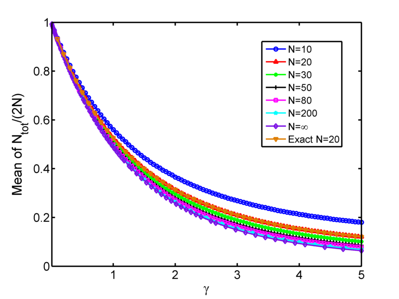
Figure 1: Mean number of stationary points as a function of $\gamma$.

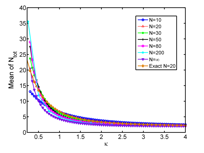
Figure 2: Mean number of stationary points as a function of $\kappa$.

In Fig. 1, the finite $N$ numerical results show a qualitatively similar trend to the asymptotic results, approaching this in a relatively fast rate as $N$ grows. The results are also compared with the exact analytic formula (5) for a fixed size $N=20$. The numerical calculations agree excellently with the analytical expressions. The same observations are valid for Fig. 2 which shows the results for the $\kappa$ regime. Here ${\mathcal{N}}(\kappa)\to 2$ for large $\kappa$, which is the limiting regime of topology trivialization as described above. In summary, these results show both the correctness of the analytical approaches for computing the mean number of stationary points in the GOE ensemble, and also the correctness of the numerical calculations from the non-Hermitian eigenvalue problem (9).

V.2 Variance of the number of real stationary points

While it is often possible to compute analytical expressions for the mean number of real solutions of a random system of equations, obtaining analytical expressions for the variances or higher order moments of the distribution is often a very difficult task, if not impossible. Indeed, for the $2$-spin spherical model, analytical expressions for the variance for both finite $N$ and $N\to\infty$ are completely unknown. It is here where numerical methods can be most useful.

By means of the non-Hermitian matrix (9), we can find all the real solutions for each sample of the $2$-spin model, and then we can straightforwardly compute the variance of the number of real solutions. This quantity, which is a measure of the fluctuations of the mean number of real solutions, is of particular relevance as it gives information on the occurrence of real versus complex solutions of the system of equations in the different regimes.

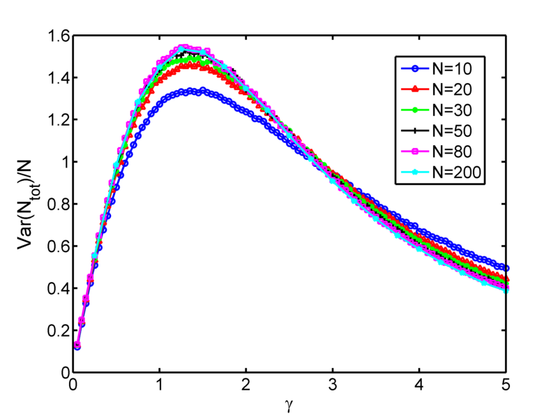
Figure 3: Variance of the number of stationary points as a function of $\gamma$.

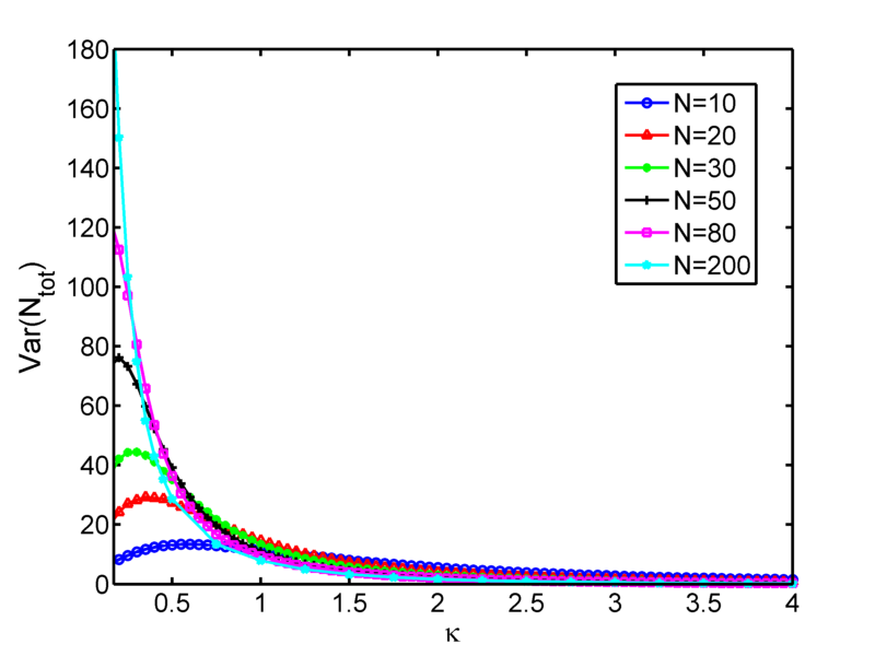
Figure 4: Variance of the number of stationary points as a function of $\kappa$.

The variance as a function of $\gamma$ and $\kappa$ for different values of $N$ is plotted in Figures 3 and 4, respectively. In Figure 3, as we increase through higher values of $N$, the variance shows a clear convergence to a well defined limiting curve, confirming our normalization of $N_{tot}$ by $N^{-1/2}$ in this context. An important open problem is to provide a theoretical justification for this normalization and the resulting limiting curve. In the $\kappa$ regime, shown in Figure 4, the number of stationary points is characterized by large fluctuations near the origin $\kappa=0^{+}$ which are quickly suppressed for increasing values of $\kappa$.

V.3 Frequencies of the no. of stationary points

Going beyond the mean and variance, we can also obtain the full distribution of the number of stationary points. The results are plotted in Figure 5 in the $\gamma$ regime for $N=75$. The plots were generated from 100,000 realizations of the matrix $A$ in equation $\eqref{eq:nonhermitianA}$. For increasing values of $\gamma$, we note the spread of the distribution behaving in accordance with the variance plot in Figure 3.

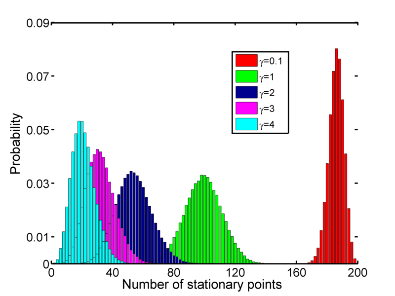
Figure 5: Probability densities of the number of stationary points for different values of $\gamma$.

As with the variance, there is not yet any analytic results about the full distribution of the number of stationary points. Its theoretical investigation may be of broader interest to practitioners of random matrix theory, as the number of real eigenvalues were investigated by several authors when the underlying matrix is composed of independent, identically distributed entries TaoVu13 or satisfies invariance EKS93 with respect to the action of an appropriate compact group. In these simpler cases, it was proven that the fluctuations of the real eigenvalue count are Gaussian when $N\to\infty$, with mean and variance of order $\sqrt{N}$. In contrast, our study shows that for the matrix $A$ in the $\gamma$-regime, the real eigenvalues instead have mean and variance of order $N$.

V.4 Distribution of global minima

In order to obtain the distribution of the global energy minimum with our methods, one simply takes the obtained values of the Lagrange multipliers (namely, the eigenvalues of the matrix $A$ in (9)) and inserts the results into (8). Then, numerically, it’s a simple task to evaluate the energy $E_{h}(\mathbf{x})$ at the $2N$ critical points and minimize over all outputs. The corresponding probability histogram is depicted in Figure 6 for $N=50$, $J=1$, $\gamma=2$ with 100,000 realizations.

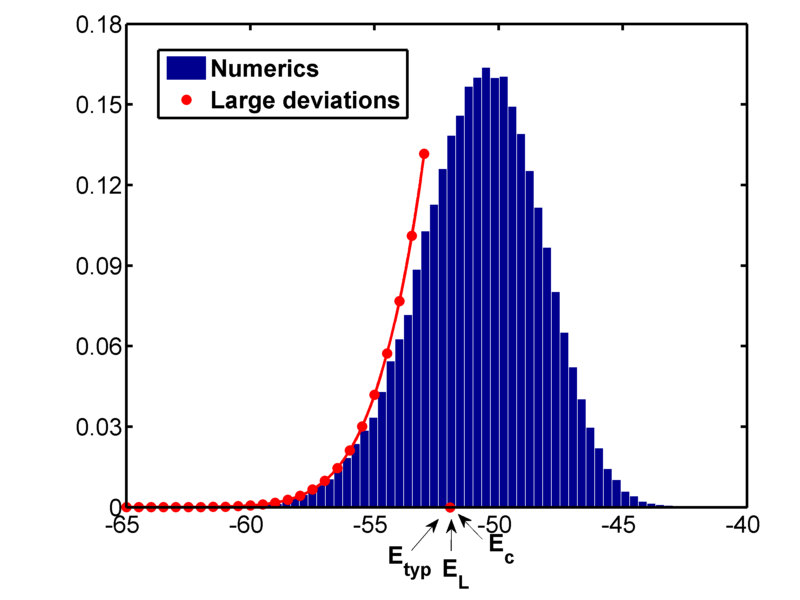
Figure 6: Probability density of $E_{\min}$ for $\gamma=2$ and $N=50$.

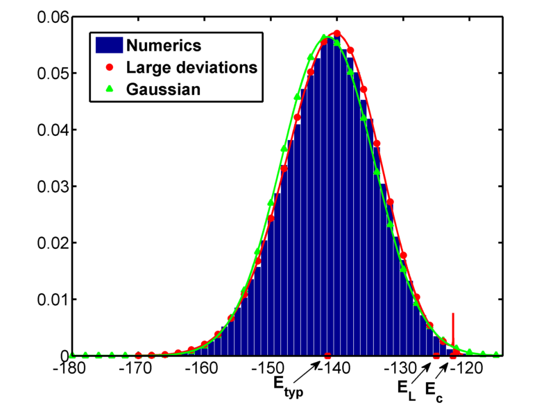
Figure 7: Probability density of $E_{\min}$ for $\sigma=1$ and $N=100$.

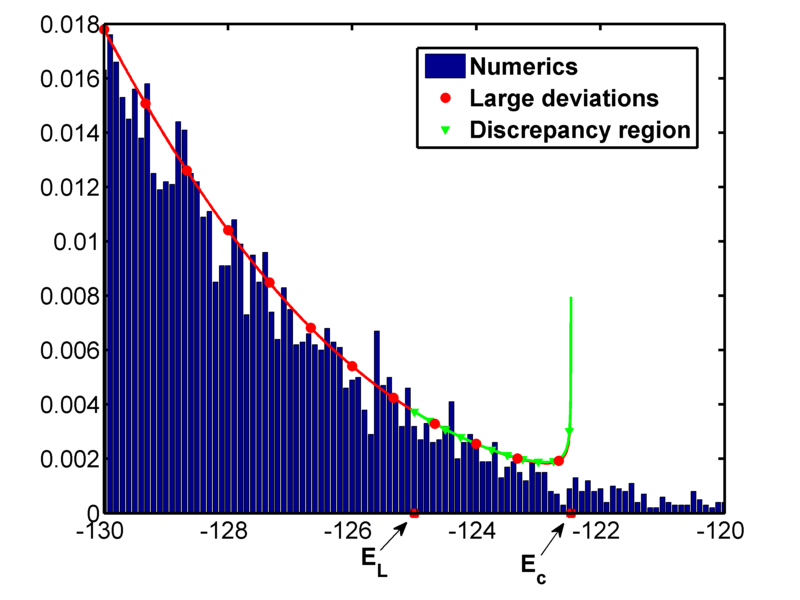
Figure 8: Probability density of $E_{\min}$ near the critical energy, again with $\sigma=1$ and $N=100$.

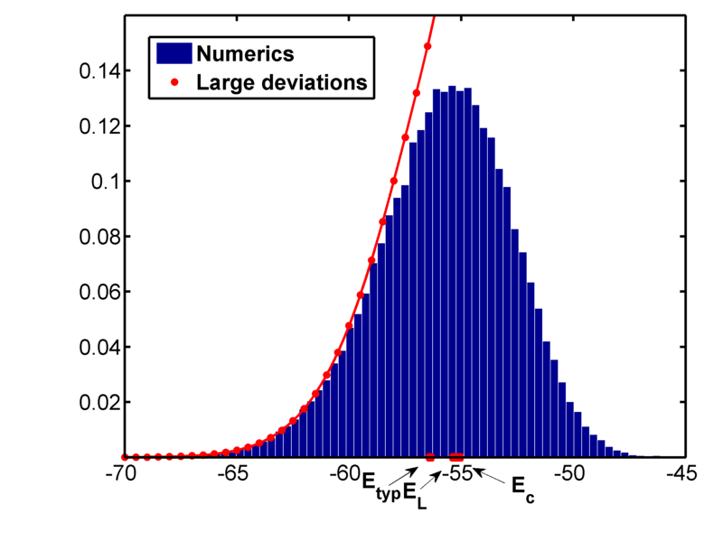
Figure 9: Probability density of $E_{\min}$ for $\kappa=1$ and $N=50$.

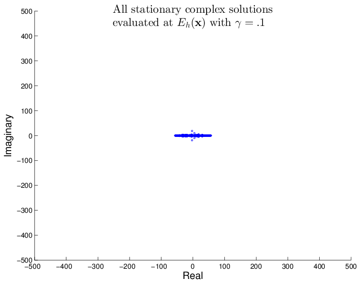
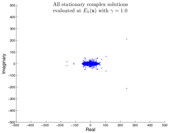
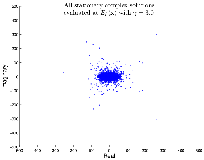
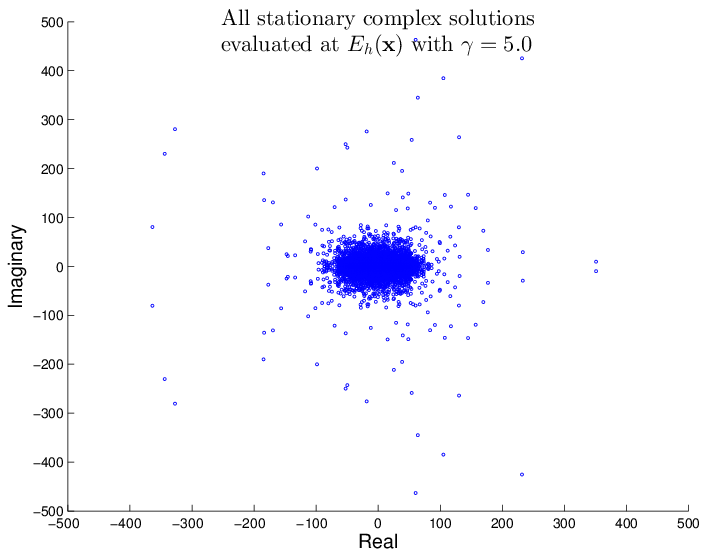
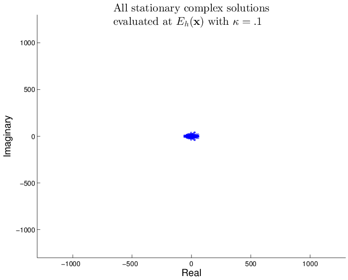
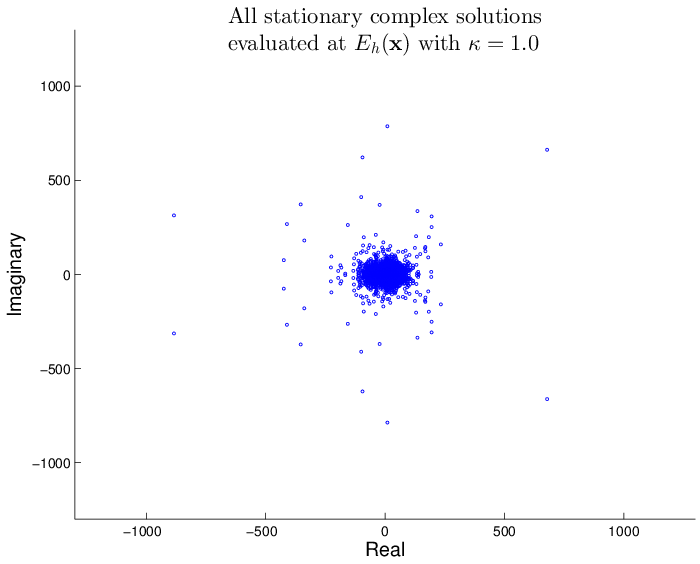
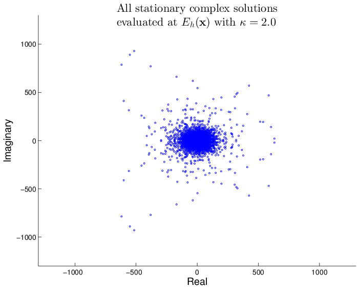
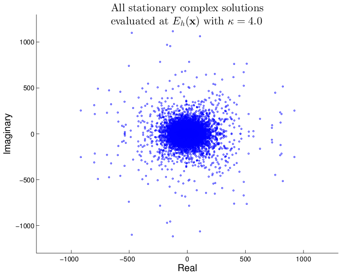
Figure 10: Plots of the real and imaginary parts of the energy function $E_{h}(\mathbf{x})$ evaluated at the complex stationary points for different values of $\gamma$ and $\kappa$.

The statistical properties of the ground state energy of the 2-spin spherical model were investigated analytically in Fyodorov-topo-triv2013 and later in DemZei14 . In Fyodorov-topo-triv2013 , a large deviations asymptotic expression for the probability density function of $E_{\min}$ was derived, valid up to a critical value of the energy $E_{c}:=-N\sqrt{\frac{1+2\sigma^{2}}{1+\sigma^{2}}}$ and depending on the parameter $E_{\mathrm{typ}}=-N\sqrt{1+\sigma^{2}}$, the typical value of $E_{\min}$. Recently the corresponding rate function was obtained rigorously in DemZei14 , revealing a surprising difference with the one obtained in Fyodorov-topo-triv2013 . Specifically, it was shown in DemZei14 that there is a different critical parameter $E_{{L}}:=-N\left(1+\frac{\sigma^{2}}{2(1+\sigma^{2})}\right)$ for which the two rate functions disagree on the interval $[E_{{L}},E_{c}]$.

In Figure 6, we plot the large deviations functional in Fyodorov-topo-triv2013 that was also proved rigorously in DemZei14 . The results show a good consistency between the two approaches in the regime of validity of large deviations $E\ll E_{{c}}$. The values of $E_{{c}}$, $E_{{L}}$ and $E_{{typ}}$ are almost identical here.

On the other hand, if we consider the regime of topology trivialization, where $\sigma>0$ is fixed, we get an almost perfect agreement with large deviations, see Figure 7, where we set $\sigma=1$, $J=1$ and $N=100$. The reason seems to be that for fixed $\sigma$, the threshold $E_{{c}}$ moves far out into the right tail of the distribution, giving a wider range of validity. The triangles show the Gaussian

$$P(E)\propto\mathrm{exp}\left(\frac{(E-E_{\mathrm{typ}})^{2}}{\sigma^{2}N}\right)$$ (10)

giving a good approximation to the tails of the distribution Fyodorov-topo-triv2013 .

For $\sigma=1$, the critical parameters also begin to separate out more and one can ask how the two large deviations expressions differ on $[E_{{L}},E_{{c}}]$. As seen in Figure 8, this difference is very small and is hard to detect numerically. Below $E_{{c}}$, the triangular data points are based on the rigorous large deviations formula in DemZei14 and circles the one in Fyodorov-topo-triv2013 . At the level of rate functions, their difference is upper bounded by $10^{-4}$ on the interval $[E_{{L}},E_{{c}}]$. Away from this interval, the two expressions are identical DemZei14 . The plot also shows that as one approaches $E_{{c}}$ the pre-exponential factor in Fyodorov-topo-triv2013 diverges and should be replaced by a different expression beyond the threshold $E_{{c}}$.

Finally, we plot the results for the $\kappa$-regime in Figure 9. Now, the large deviation expressions gives an agreement somewhere in between the last two regimes, as expected from the fact that $\sigma_{\gamma}\ll\sigma_{\kappa}\ll 1$, where $\sigma_{\gamma}$ and $\sigma_{\kappa}$ denote the $\sigma$ values corresponding to the $\gamma$ and $\kappa$ regimes respectively.

V.5 Complex Stationary Points

As stated before, the NPHC method finds all complex solutions of (4). Since, with probability $1$, there are always $2N$ complex solutions for any random sample, only the number of real solutions varies with $\gamma$ and $\kappa$. In other words, while increasing $\gamma$ and $\kappa$, some of the real stationary points become complex solutions. One way of studying this phenomenon is by plotting real vs imaginary parts of $E_{h}(\textbf{x})$, see Figure 10. The plots show that at small $\gamma$ and $\kappa$, the imaginary part of $E_{h}(\textbf{x})$ evaluated at all the $2N$ complex stationary points is zero. As the parameters increase, the imaginary parts of $E_{h}(\textbf{x})$ increases meaning that some of the real solutions became nonreal.

VI Discussion and Conclusion

Exploring potential energy landscapes of various models arising in physics and chemistry is a very active area of research in different fields of science and mathematics. Recently, a curious feature of the potential energy landscapes of a class of statistical mechanics models has been observed, namely, topology trivialization: while varying one or more parameters of the potential, either continuously or varying the variance of the random distribution the parameter values are drawn from, the mean number of real stationary points of the potential varies from $O(1)$ to $O(N)$ or even higher. In the former case, the topology of the $N$-dimensional landscape can be viewed as being trivialized. These two phases are shown to be related to phase transitions of the systems. In this work we have done a numerical study of the topology trivialization scenario in the $2$-spin spherical model. While the mean number of real stationary points can be computed analytically using random matrix theory tools, computing other quantities such as the variance of the number of real stationary points and the full distribution are prohibitively difficult for current analytical computation techniques.

We used two numerical methods, namely, the numerical polynomial homotopy continuation (NPHC) method and non-Hermitian matrix method. One first translates the problem of finding stationary points into an algebraic geometry problem of solving a system of polynomial equations. This interpretation yields an upper bound on the number of complex solutions, namely $2N$ which is equal to the known upper bound on the number of real solutions for this system. In fact, $2N$ is equal to the number of complex solutions, with probability $1$, and only the number of real solutions varies with each instance. Hence, we have found a more general result for the number of solutions of the $2$-spin model.

The second method, though apparently only specific to the $2$-spin case, works more efficiently in this case by finding all the real solutions for a given random instance and hence giving an opportunity to reach much higher dimension $N$ and sample size. The method does not find complex solutions which were analyzed using the NPHC method.

With the two powerful methods at our disposal, we first reproduced the analytical predictions on the mean number of real solutions with an excellent agreement. We also addressed the issue of fluctuations of the number of solutions, showing that for the $\gamma$-regime, the variance of the number of critical points is of order $N$ as $N\to\infty$. To show this analytically seems to us an important open problem. Little is known in general about fluctuations of the number of critical points in random Gaussian fields, although in a different context results in this direction were obtained in KleAga12 .

We also investigated statistics of the global energy minimum $E_{\min}$. When $\sigma>0$ is fixed and large enough that $E_{c}\gg E_{\mathrm{typ}}$ (corresponding to the regime of topology trivialization), our findings give a strong agreement with the heuristic arguments in Fyodorov-topo-triv2013 . Remarkably, it seems that in this regime, the entire distribution of $E_{\min}$ yields precise agreement with the large deviations expression in Fyodorov-topo-triv2013 . In the $\gamma$ and $\kappa$ regimes, the agreement with large deviation theory is limited to the left tail of the distribution. The reason seems to be that when $\sigma\to 0$, the critical energy threshold $E_{c}$ moves further into the bulk of the distribution and we know that the pre-exponential factors from Fyodorov-topo-triv2013 are not valid if $E>E_{c}$. Analytical understanding of the statistics of $E_{\min}$ in the right tail for the $\gamma$ and $\kappa$ regimes therefore remains an outstanding issue.

We note that the topology trivialization phenomenon, at least in the simple case of continuously varying parameters, shares a deep connection with Catastrophe theory, which is now absorbed in a more general mathematical framework of singularity theory and bifurcation theory. From Catastrophe theory, it is known that varying the parameters of the potential continuously the real stationary points may appear or disappear, or change their stability properties wales2001microscopic ; bogdan2004new . In Refs. Kastner:2011zz ; Mehta:2012qr ; Mehta:2014comm , it was observed that while continuously varying the parameter of the two-dimensional nearest neighbor $\phi^{4}$ model, some of the real stationary points would merge to become complex solutions and vice versa.

The fact that the topology trivialization occurs when varying the variance of the random distributions from which the parameters are drawn, rather than varying the parameters themselves, makes such a description more subtle. In the present work, however, we have observed that a similar phenomenon of real stationary points transforming to complex and vice versa is occurring in the $2$-spin model too when varying $\gamma$ and $\kappa$.

Another description of the topology trivialization phenomenon may come from our algebraic geometry interpretation of the $2$-spin model: for a simple system $ax^{2}+bx+c=0$, where $a,b$ and $c$ are real parameters, the discriminant $b^{2}-4ac$ decomposes the 3D parameter space in to three phases, i.e., no real roots, two distinct real roots and double roots. Thus, the number of real solutions goes from the highest possible to zero. Similarly, a discriminant can be defined for multivariate polynomials case and a similar classification of the parameter space based on the number of real solutions can be worked out using the so-called discriminant variety method gel1994fand ; lazard2007solving ; hanan2010stability . From this, one can study the topology trivialization fairly straightforwardly for the case of continuously varying parameters. However, the case of varying variances of the random distributions of the parameters is still subtle and largely unexplored even from the Mathematics point of view.

Thus, we anticipate that our results will merge the topology trivialization phenomenon with the emerging mathematical areas called Statistical Topology, or perhaps inspire a new subbranch that may be called statistical catastrophe theory or stastical discriminant variety.

We also note that for higher $N$, numerical instabilities become profound when finding stationary points of the $p$-spin model using the above numerical methods. To resolve this issue, one can employ, for example, Smale’s alpha theorem to certify if a numerical approximate is provably within the quadratic convergence region of the nearby exact root. Combining this certification with the NPHC method then gives a result equivalent to the exact result for each random instance Mehta:2013zia ; Mehta:2014gia . In the future, we plan to use this combination to prove concrete results for higher values of $N$.

- (1) Y. Fyodorov and P. Doussal J. Stat. Phys. 154, 466-490 (2014).
- (2) A. Dembo and O. Zeitouni, “Matrix optimization under random external fields”, ARXIV:1409.4606.
- (3) Y. Fyodorov , “High dimensional random fields and Random Matrix Theory”, ARXIV:1307.2379.
- (4) G. Wainrib and J. Touboul Phys. Rev. Lett., 110, 118101 (2013).
- (5) T. Tao and V. Vu, “Random matrices: Universality of local spectral statistics of non-Hermitian matrices”, ARXIV:1206.1893.
- (6) D.J. Wales, Energy Landscapes, Cambridge University Press, 2004.
- (7) M. Kastner, Rev. Mod. Phys. 80, 167 (2008).
- (8) D. Mehta and M. Kastner, Annals Phys. 326, 1425 (2011).
- (9) A. Auffinger, G. Ben Arous and C. Cerny, Comm. Pure. Appl. Math. 66, 165 (2013).
- (10) P. J. Forrester, J. Phys. A: Math. Theor. 45, 075206 (2012).
- (11) A. Klein and O. Agam , J. Phys. A: Math. Theor. 45, 025001 (2012).
- (12) D. Mehta, Ph.D. Thesis, The Uni. of Adelaide, Australasian Digital Theses Program (2009).
- (13) D. Mehta, A. Sternbeck, L. von Smekal, and A.G. Williams, PoS QCD-TNT09, 025 (2009).
- (14) D. Mehta, Phys.Rev. E (R) 84, 025702 (2011).
- (15) D. Mehta, Adv.High Energy Phys. 2011, 263937 (2011).
- (16) M. Kastner and D. Mehta, Phys.Rev.Lett. 107, 160602 (2011).
- (17) M. Maniatis and D. Mehta, Eur.Phys.J.Plus 127, 91 (2012).
- (18) D. Mehta, Y.-H. He, and J.D. Hauenstein, JHEP 1207, 018 (2012).
- (19) C. Hughes, D. Mehta, and J.-I. Skullerud, Annals Phys. 331 188 (2013).
- (20) D. Mehta, J.D. Hauenstein, and M. Kastner, Phys.Rev. E85, 061103 (2012).
- (21) D. Mehta, T. Chen, J. D. Hauenstein and D. J. Wales Newton Homotopies for Sampling Stationary Points of Potential Energy Landscapes. J. Chem. Phys. , in press (2014).
- (22) D. Martinez-Pedrera, D. Mehta, M. Rummel and A. Westphal, JHEP 1306, 110 (2013)
- (23) Y.-H. He, D. Mehta, M. Niemerg, M. Rummel, and A. Valeanu, JHEP 1307, 050 (2013).
- (24) D. Mehta, D.A. Stariolo and M. Kastner, Phys. Rev. E 5 87 052143 (2013).
- (25) B. Greene, D. Kagan, A. Masoumi, D. Mehta, E. J. Weinberg and X. Xiao, Phys. Rev. D 88, 026005 (2013).
- (26) D. Mehta, N. S. Daleo, J. D. Hauenstein and C. Seaton, Phys. Rev. D 90, 054504 (2014)
- (27) J. D. Hauenstein, A. Lerario, E. Lundberg and D. Mehta, Experiments on the zeros of harmonic polynomials using certified counting. J. Exp. Math. In press (2014). arXiv:1406.5523.
- (28) D.J. Bates, J.D. Hauenstein, A.J. Sommese, and C.W. Wampler. Numerically solving polynomial systems with Bertini, volume 25. SIAM, 2013.
- (29) D.J. Bates, J.D. Hauenstein, A.J. Sommese, and C.W. Wampler. Bertini: Software for Numerical Algebraic Geometry. bertini.nd.edu.
- (30) A. Edelman, E. Kostlan and M. Shub, How Many Eigenvalues of a Random Matrix are real?, Journal of the American Mathematical Society 7, 1994.
- (31) Y. Fyodorov, Complexity of Random Energy Landscapes, Glass Transition, and Absolute Value of the Spectral Determinant of Random Matrices, Phys. Rev. Lett 92, 240601, (2004).
- (32) A.J. Sommese and C.W. Wampler, The numerical solution of systems of polynomials arising in Engineering and Science, World Scientific Publishing Company, 2005.
- (33) K. Kowalski and K. Jankowski, Phys. Rev. Lett. 81, 1195 (1998).
- (34) A.J.W. Thom and M. Head-Gordon, Phys. Rev. Lett. 101, 193001 (2008).
- (35) L. Piela, J. Kostrowicki, and H.A. Scheraga, J. Phys. Chem. 93, 3339 (1989).
- (36) C. W. Wampler Bézout number calculations for multi-homogeneous polynomial systems., Applied Math. and Comp. 1992
- (37) D. J. Wales Science, 293 5537, 2067 (2001).
- (38) T. V. Bogdan and D. J. Wales, J. Chem. Phys. , 120 23, 11090 (2004).
- (39) I. M. Galfand, M. M. Kapranov, and A. V. Zelevinsky, Discriminants, resultants, and multidimensional determinants, Mathematics: Theory & Applications (1994). Birkhäuser Boston Inc., Boston, MA.
- (40) D. Lazard and F. Rouillier, J. Sym. Comp. 42 6, 636 (2007).
- (41) W. Hanan, D. Mehta, G. Moroz and S. Pouryahya. ”Extended abstract” published in the Joint Conference of ASCM2009 and MACIS2009, Japan, 2009. arXiv:1001.5420.
- (42) D. Mehta, J.D. Hauenstein and D.J. Wales, J. Chem. Phys., 138, 171101 (2013).
- (43) D. Mehta, J. D. Hauenstein and D. J. Wales, J. Chem. Phys. 140, 224114 (2014).