VLT/UVES observations of peculiar $\alpha$ abundances in a sub-DLA at $z\approx 1.8$ towards the quasar B1101$-$26

We present a detailed analysis of chemical abundances in a sub-damped Lyman $\alpha$ absorber at $z=1.839$ towards the quasar B1101$-$26, based on a very-high-resolution ($R\sim 75,000$) and high-signal-to-noise (S/N $>100$) spectrum observed with the UV Visual Echelle spectrograph (UVES) installed on the ESO Very Large Telescope (VLT). The absorption line profiles are resolved into a maximum of eleven velocity components spanning a rest-frame velocity range of $\approx 200$ km s^-1. Detected ions include C ii, C iv, N ii, O i, Mg i, Mg ii, Al ii, Al iii, Si ii, Si iii, Si iv, Fe ii, and possibly S ii. The total neutral hydrogen column density is $\log N($H i$)=19.48\pm 0.01$. From measurements of column densities and Doppler parameters we estimate element abundances of the above-given elements. The overall metallicity, as traced by [O i/H i], is $-1.56\pm 0.01$. For the nitrogen-to-oxygen ratio we derive an upper limit of [N i/O i] $\leq-0.65$, which suggests a chemically young absorption line system. This is supported by a supersolar $\alpha$/Fe ratio of [Si ii/Fe ii] $\approx 0.5$. The most striking feature in the observed abundance pattern is an unusually high sulphur-to-oxygen ratio of $0.69\leq$ [S ii/O i] $\leq 1.26$. We calculate detailed photoionisation models for two subcomponents with Cloudy, and can rule out that ionisation effects alone are responsible for the high S/O ratio. We instead speculate that the high S/O ratio is caused by the combination of several effects, such as specific ionisation conditions in multi-phase gas, unusual relative abundances of heavy elements, and/or dust depletion in a local gas environment that is not well mixed and/or that might be related to star-formation activity in the host galaxy. We discuss the implications of our findings for the interpretation of $\alpha$-element abundances in metal absorbers at high redshift.

1 Introduction

The formation and evolution of galaxies are important aspects for our understanding of the Universe and its structure. In particular, the reconstruction of the chemical history of galaxies and the metal content in the early Universe are fundamental steps to understanding these basic processes. One efficient way to investigate them is to study the distribution and chemical composition of gas inside and outside of galaxies in the interstellar and intergalactic medium (ISM and IGM) at different redshifts. This gas can be studied through intervening absorption line systems detected in the spectra of bright background sources, for example quasars. This approach provides the advantage of being unbiased with respect to distance, luminosity, and morphology of the host galaxies, whereas the observation of the faint starlight is exceedingly difficult.

Intervening absorbers are classified into four categories according to their neutral hydrogen column density (and, consequently, their relation to galaxies). Intergalactic gas clouds with column densities of neutral hydrogen less than $N$(H i) $\lesssim 10^{17}$ cm^-2 are called Lyman $\alpha$ forest systems (see e.g. Meiksin 2009). These absorbers are believed to predominantly trace the low-density intergalactic medium (IGM) beyond the virial radii of galaxies. The so-called Lyman limit systems (LLS) have column densities up to $10^{19}\mathrm{\,cm}^{-2}$ and are believed to mostly arise in the the circumgalactic medium (CGM) of galaxies. These systems might be important tracers of gas infall and outflow processes that circulate the gas around galaxies (Crighton et al. 2013; van de Voort et al. 2012; Rudie et al. 2012; Faucher-Giguère & Kereš 2011; Fumagalli et al. 2011) and could therefore be a significant metal reservoir (Prochaska et al. 2006). Absorption line systems with neutral hydrogen column densities $>2\times 10^{20}$ cm^-2 are called damped Lyman $\alpha$ systems (DLAs). The sub-damped Lyman $\alpha$ systems (sub-DLAs) comprise the transition between Lyman limit systems and DLAs with column densities $10^{19}$ cm${}^{-2}\leq N($H i$)\leq 2\times 10^{20}$ cm^-2 (Dessauges-Zavadsky et al. 2003; Péroux et al. 2003). Because of their large neutral hydrogen content, DLAs and sub-DLAs are believed to be associated with the inner regions of galaxies (e.g. with the gas disks of spirals).

Absorption-line measurements indicate that DLA systems dominate the neutral gas content of the Universe at $z>1$ (Lanzetta et al. 1995; Rao & Turnshek 2000). Studies of DLAs are in line with the idea that these systems are the progenitors of present-day galaxies (e.g. Møller et al. 2013; Rafelski et al. 2012, 2011; Yin et al. 2011; Zwaan et al. 2005; Wolfe et al. 2005; Boissier et al. 2003; Fritze-v. Alvensleben et al. 2001; Salucci & Persic 1999; Prochaska & Wolfe 1997). In contrast to DLAs, sub-DLAs have lower neutral gas column densities, but they are generally considered to be more metal rich than DLAs (Som et al. 2013; Meiring et al. 2009; Péroux et al. 2007). However, ionisation corrections may be significant for these systems and notably alter the metallicity estimates. Nonetheless, for a given metallicity, sub-DLAs have lower metal column densities than DLAs owing to the low H i column densities. This allows us to accurately measure the abundance of the most common elements like oxygen and carbon without facing the problem of line saturation. Accurate abundance measurements of metals are particularly important to learn about the chemical enrichment of the gas inside and outside of galaxies, because they constrain the conditions for early nucleosynthesis in the Universe.

As certain types of enrichment processes cause a specific abundance pattern in the ISM and IGM, we can deduce different types of stellar explosions and physical processes from the abundance measurements in absorption line systems. In order to explain the metal-abundance patterns in DLAs, two complementary effects are often brought up: (1) the nucleosynthetic enrichment from Type II supernovae (SNe) and (2) an interstellar medium-like (ISM-like) dust-depletion pattern. A typical Type II SN enrichment pattern shows an overabundance of O relative to N, an underabundance of elements with odd atomic number compared to elements with even atomic number (e.g. Mn/Fe and Al/Si), and an overabundance of $\alpha$-elements (e.g. O, Si, S) relative to iron peak elements (e.g. Cr, Mn, Fe, Ni) (see Lu et al. 1996, and references therein). The last is caused by the relatively quick production of $\alpha$-capture elements and some iron peak elements in Type II SNe, while at later times a dominant production of the iron peak elements comes from Type Ia SNe whose precursors evolve more slowly than the massive stars that cause SNe Type II. The production of nitrogen, on the other hand, is less well understood, but it is assumed that the production is dominated by intermediate-mass stars (Henry et al. 2000).

Comprehensive studies of DLAs, performed for example by Lu et al. (1996) and Prochaska & Wolfe (1999), found abundance patterns that are broadly consistent with a combination of SN Type II enrichment and dust-depletion, but at the same time they find exceptions that cannot be explained by these two effects. Som et al. (2013) confirmed suggestions for sub-DLAs being more metal-rich than DLAs and evolving faster. Besides, abundance ratios of [Mn/Fe] in their study suggest a difference in the stellar populations for the galaxies traced by DLAs and sub-DLAs. It seems that, even though many observational studies of DLAs and sub-DLAs have been pursued (e.g. Ledoux et al. 2003; Dessauges-Zavadsky et al. 2003; Som et al. 2013), the abundance patterns lack a convincing single interpretation. Furthermore, the characteristic of the influence of dust-depletion on the observed abundance ratios (Vladilo et al. 2011) is an ongoing issue of debate.

Since the origin of sub-DLAs with respect to the location of the star-forming inner regions of galaxies is unclear, these systems have been largely ignored until recently. However, detailed studies of this class of absorbers are advantageous and desirable, not only for the observational reasons mentioned above. One major drawback that hampers the interpretation of chemical abundances in LLS, sub-DLAs and DLAs is the often complex velocity-component structure in the absorbers. This velocity structure reflects the complex spatial distribution of the different gas phases in and around galaxies at pc and kpc scales. Since a typical quasar sightline that contains a sub-DLA or DLA passes both the inner (star-forming) region of a galaxy and the outer circumgalactic environment, it cannot be readily expected that the different absorption components contain gas with one and the same chemical enrichment pattern. While most of the previous studies of DLAs and sub-DLAs largely ignore this aspect, partly because of limitations in spectral resolution and signal-to-noise (S/N) in the data, some detailed studies on kinematically complex DLAs and sub-DLAs at high $z$ indeed indicate a non-uniform abundance pattern within the absorbers (Crighton et al. 2013; Prochter et al. 2010; D’Odorico & Petitjean 2001), e.g. as part of merger processes (Richter et al. 2005). Such accurate measurements require very high-resolution spectra of quasars with high S/N ($\gtrsim 50$), but these are sparse and detailed analyses of their absorption line systems are even rarer.

To improve our understanding of the chemical enrichment pattern within DLAs and sub-DLAs at high redshift, we present in this paper a detailed analysis of a complex sub-DLA at $z=1.839$ in the optical spectrum of the quasar B1101$-$26. Our analysis is based on a very-high-spectral-resolution ($R=75\,000$) and high-signal-to-noise ratio (S/N $\sim 100$) spectrum of QSO B1101$-$26 taken with VLT/UVES. After presenting our data set and analysis method in Sec. 3, we present the results of the absorption-line fitting and the photoionisation models in Sec. 4. In Sec. 5, we give a detailed discussion of our findings and summarise our study in Sec. 6. Throughout the paper we use the list of atomic data provided by Morton (2003).

2 The sub-DLA towards QSO B1101$-$26

The optical spectrum of QSO B1101$-$26, (other name: 2MASS J110325$-$264515, $m_{V}=16\aas@@fstack{m}02$, $z_{\text{em}}=2.145$) contains a prominent sub-DLA at $z_{\text{abs}}=1.839$ that exhibits a complex velocity-component structure spanning more than $200$ km s^-1 in the absorber restframe. This sub-DLA has been subject of earlier studies, e.g. by Petitjean et al. (2000) and by Dessauges-Zavadsky et al. (2003). These previous studies used early observational data at high spectral resolution ($R\sim 45,000$) obtained in 2000 with the UV-Visual Echelle Spectrograph (UVES) installed on ESO Very Large Telescope (VLT) as part of the UVES Science Verification. From the analysis of these data, Dessauges-Zavadsky et al. (2003) derived a total neutral hydrogen column density of $\log N$(H i) $=19.50\pm 0.05$ in the sub-DLA from a fit of the Ly $\alpha$ line. In their dataset, that has an average velocity resolution of $5-7$ km s^-1, they could resolve the absorption pattern of the weakly ionised species into 11 subcomponents, whereas the highly ionised species have been resolved into six subcomponents. Moreover, Dessauges-Zavadsky et al. (2003) have measured the column densities in the sub-DLA for 11 ions and seven elements (Si, O, S, C, Al, Fe, Mg) that they could identify. For all these elements, they have computed the abundances using solar abundances provided by Grevesse & Sauval (1998). For example, they have confirmed the measurements of Petitjean et al. (2000) for the iron abundance being [Fe/H]$=-1.49\pm$0.05 and they have determined an oxygen (= alpha) abundance of [O/H]$=-1.78\pm 0.12$ that surprisingly is significantly lower than that of Fe. However, the true velocity structure in the gas is possibly not fully resolved at the given spectral resolution. Concludingly, the true Doppler parameters ($b$-values) in the individual (unresolved) components may be significantly lower than what has been estimated previously and, thus, the column densities could be underestimated. Therefore, the limited spectral resolution and S/N leads to systematic uncertainties for the derived abundances. A more detailed analysis of this complex absorption line system with higher-resolution data is possible with the data set used here and can provide deeper insights into the metal enrichment at high redshift, based on more accurate abundance measurements.

3 Observations, data handling, and analysis method

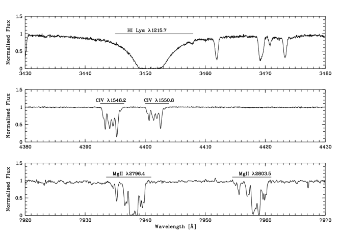
Figure 1: Portion of UVES spectrum of QSO B1101$-$26. In the upper panel, the H i Ly $\alpha$ absorption in the sub-DLA at $z=1.839$ is shown. The middle and lower panel show the C iv and Mg ii absorption lines of the same absorption line system, respectively.

The spectral data used in this study have been obtained with UVES/VLT in February 2006 as part of the VLT observing programme 076.A-0463(A). This programme aims at constraining the cosmological variability of the fine-structure constant by observing metal absorption-line systems in quasar spectra (PI/Col: Lopez/ Molaro/ Centurión/ Levshakov/ Bonifacio/ D’Odorico). QSO B1101$-$26 was observed through a $0.5$ arcsec slit under good seeing conditions ($\lesssim 1$ arcsec) during the run. The total integration time was 100 261 s. The data are of high spectral resolution ($R\sim 75\,000$ or 4 km s^-1 FWHM) and exhibit an excellent S/N of $\sim 100$, on average ($45$ at $3550$ Å, $140$ at $4400$ Å). The raw data were reduced and normalised to the local continuum of the quasar as part of the UVES Spectral Quasar Absorption Database (SQUAD; PI: Michael T. Murphy) using a modified version of the UVES pipeline. The reduction includes flat-fielding, bias- and sky-subtraction, and a relative wavelength calibration. The final combined spectrum covers a wavelength range of $3050-10\,430$ Å. A representative portion of the UVES spectrum of QSO B1101$-$26 is displayed in Fig. 1, showing selected absorption lines of the sub-DLA system at $z=1.839$. The data are publicly available in the UVES database within ESO’s Science Archive Facility.

The high resolution and high S/N of the new UVES spectrum of QSO B1101$-$26 enables us to identify absorption lines arising from 14 different ions, namely H i, C ii, C iv, N ii, O i, Mg i, Mg ii, Al ii, Al iii, Si ii, Si iii, Si iv, Fe ii, and possibly S ii. We have analysed the spectrum using the FITLYMAN package implemented in MIDAS (Fontana & Ballester 1995). This routine uses a $\chi^{2}$-minimisation algorithm for multi-component Voigt-profile fitting to derive column densities, $N$, and Doppler-parameters, $b$, taking into account the instrumental line-spread function (LSF). Because different lines from the same ion are fitted simultaneously, $b$-values obtained from the fit can be smaller than the velocity resolution of the instrument, as the information on the relative line strengths enters the determination of $b$ in the fit. This also means that even at this high spectral resolution the absorption profiles may be unresolved and the true velocity-component structure remains uncertain. Consequently, the physical interpretation of the derived $b$-values (e.g. in terms of thermal broadening processes) remains afflicted with systematic uncertainties.

4 Results and discussion

4.1 Velocity structure

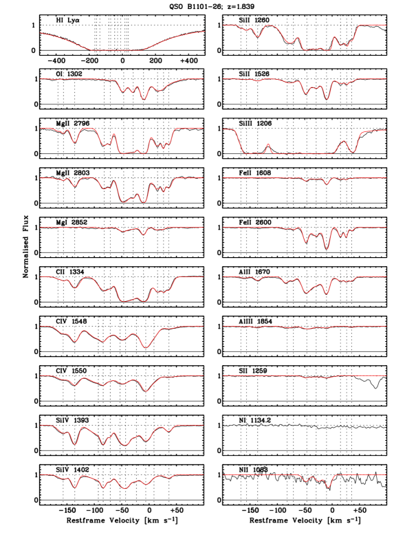
Figure 2: Absorption profiles of H i, C ii, C iv, N i, N ii, O i, Mg i, Mg ii, Al ii, Al iii, Si ii, Si iv, S ii, and Fe ii for the $z=1.839$ sub-DLA. The individual absorption components are indicated by the vertical dashed lines. The velocity scale refers to the $z=1.839$ restframe. The multi-component Voigt profile fits are overlayed in red. Parameters of the fit can be found in Table 1.

The component structures in the $z=1.839$ absorber for neutral and weakly ionised species and highly ionised species were analysed separately, because these ions usually do not arise in the same gas phase (Crighton et al. 2013; Milutinovic et al. 2010; Fox et al. 2007b; Wolfe et al. 2005) (see Fig. 2). The Mg ii absorption line is a good representative for the velocity structure of the weakly ionised species, because it represents a strong atomic transition that is found in a regime with a very high S/N and is mostly unaffected by blending. Therefore, we have used the velocity-component structure of Mg ii as template for all weakly ionised species to obtain comparable column densities for the individual components, but we allow a $\Delta\lambda=0.05$ Å wavelength displacement ($\simeq 2$ pixels) in the absolute positions of the absorption components during the fitting process. Because of the large number of absorption lines and components, a simultaneous fit for all of them has not been possible. However, multiplets of the same ion have been fitted simultaneously, which allows us to determine the fitting parameters with high accuracy. For weak or undetected absorption features, we determine the limiting equivalent width based on the local S/N and considering a $3\sigma$ detection limit for unsaturated line absorption. A representative multi-component fit of the Al ii $\lambda$1670 absorption line is shown in Fig. 3. The highly ionised species C iv and Si iv have been fitted simultaneously altogether. Therefore, they have a common velocity structure by definition.

Table 1: Component structure, column densities, and Doppler parameters for the $z=1.839$ absorber towards QSO B1101$-$26

No	$v_{\text{rel}}$ [km s-1]	Ion A	$\log N$(A)	$b$ [km s-1]
1	$-166.4$	C ii	$12.61\pm 0.05$	$9.5\pm 0.6$
		N ii	$-$	$-$
		O i	$12.45\pm 0.08(0.09)$	$10.7\pm 2.3$
		Mg i	$-$	$-$
		Mg ii	$11.50\pm 0.13$	$6.3\pm 2.0$
		Al ii	$10.79\pm 0.06$	$5.3\pm 0.9$
		Al iii	$10.94\pm 0.22(0.22)$	$7.9\pm 4.5$
		Si ii	$11.28\pm 0.12$	$3.6\pm 1.1$
		S ii	$-$	$-$
		Fe ii	$-$	$-$
2	$-156.3$	C ii	$12.35\pm 0.09$	$4.8\pm 0.5$
		N ii	$-$	$-$
		O i	$12.08\pm 0.12(0.12)$	$4.2\pm 1.1$
		Mg i	$-$	$-$
		Mg ii	$11.63\pm 0.09$	$4.4\pm 0.7$
		Al ii	$10.55\pm 0.09$	$3.9\pm 1.0$
		Al iii	$-$	$-$
		Si ii	$11.94\pm 0.04$	$7.9\pm 0.9$
		S ii	$-$	$-$
		Fe ii	$-$	$-$
3	$-135.9$	C ii	$13.36\pm 0.00$	$9.8\pm 0.1$
		N ii	$-$	$-$
		O i	$-$	$-$
		Mg i	$-$	$-$
		Mg ii	$12.40\pm 0.01$	$7.2\pm 0.1$
		Al ii	$11.44\pm 0.01$	$7.0\pm 0.2$
		Al iii	$11.43\pm 0.07(0.08)$	$8.9\pm 1.7$
		Si ii	$12.39\pm 0.01$	$8.2\pm 0.2$
		S ii	$-$	$-$
		Fe ii	$-$	$-$
4	$-82.1$	C ii	$13.67\pm 0.01$	$14.6\pm 0.2$
		N ii	$-$	$-$
		O i	$12.50\pm 0.08(0.09)$	$11.0*$
		Mg i	$10.80\pm 0.06(0.13)$	$11.0*$
		Mg ii	$12.65\pm 0.02$	$9.6\pm 0.4$
		Al ii	$11.69\pm 0.01$	$7.2\pm 0.3$
		Al iii	$11.69\pm 0.05(0.06)$	$12.0\pm 1.7$
		Si ii	$12.37\pm 0.13$	$17.4\pm 0.8$
		S ii	$-$	$-$
		Fe ii	$11.80\pm 0.04(0.05)$	$7.9\pm 1.1$
5	$-70.8$	C ii	$12.38\pm 0.05$	$2.7\pm 0.4$
		N ii	$-$	$-$
		O i	$12.81\pm 0.05(0.06)$	$8.5\pm 1.3$
		Mg i	$10.20\pm 0.17(0.21)$	$5.0*$
		Mg ii	$12.06\pm 0.05$	$3.7\pm 0.3$
		Al ii	$11.35\pm 0.03$	$5.4\pm 0.3$
		Al iii	$-$	$-$
		Si ii	$12.83\pm 0.04$	$14.5\pm 0.2$
		S ii	$-$	$-$
		Fe ii	$11.75\pm 0.04(0.05)$	$5.0*$
6	$-46.3$	C ii	$14.22\pm 0.03$	$10.3\pm 0.3$
		N ii	$13.14\pm 0.07(0.07)$	$7.4*$
		O i	$13.83\pm 0.01(0.03)$	$8.3\pm 0.2$
		Mg i	$11.36\pm 0.03(0.12)$	$9.6\pm 0.7$
		Mg ii	$13.37\pm 0.02$	$8.8\pm 0.2$
		Al ii	$12.25\pm 0.01$	$8.7\pm 0.1$
		Al iii	$11.96\pm 0.05(0.06)$	$12.6\pm 1.7$
		Si ii	$13.33\pm 0.01$	$7.0\pm 0.1$
		S ii	$13.28\pm 0.08$	$7.4\pm 1.5$
		Fe ii	$12.78\pm 0.01(0.03)$	$5.7\pm 0.1$
7	$-29.0$	C ii	$13.88\pm 0.06$	$9.7\pm 1.1$
		N ii	$13.17\pm 0.07(0.07)$	$8.5*$
		O i	$13.77\pm 0.01(0.03)$	$6.9\pm 0.2$
		Mg i	$11.03\pm 0.11(0.16)$	$10.9\pm 2.8$
		Mg ii	$13.01\pm 0.03$	$8.0\pm 0.6$
		Al ii	$12.23\pm 0.02$	$15.6\pm 0.9$
		Al iii	$11.13\pm 0.47(0.47)$	$8.5*$
		Si ii	$13.26\pm 0.01$	$11.4\pm 0.4$
		S ii	$13.13\pm 0.19$	$9.2\pm 2.5$
		Fe ii	$12.67\pm 0.01(0.03)$	$9.8\pm 0.3$

Table 1 – Continued
No	$v_{\text{rel}}$ [km s-1]	Ion A	$\log N$(A)	$b$ [km s-1]
8	$-10.2$	C ii	$14.16\pm 0.01$	$9.1\pm 0.2$
		N ii	$13.44\pm 0.04(0.04)$	$6.4*$
		O i	$14.15\pm 0.00(0.03)$	$7.4\pm 0.1$
		Mg i	$11.47\pm 0.02(0.12)$	$6.0\pm 0.3$
		Mg ii	$13.35\pm 0.02$	$6.7\pm 0.2$
		Al ii	$12.23\pm 0.01$	$6.2\pm 0.1$
		Al iii	$11.66\pm 0.11(0.11)$	$10.7\pm 3.5$
		Si ii	$13.55\pm 0.00$	$6.0\pm 0.1$
		S ii	$13.56\pm 0.06$	$13.2\pm 0.9$
		Fe ii	$13.10\pm 0.0(0.03)$	$5.3\pm 0.1$
9	15.4	C ii	$13.58\pm 0.01$	$10.2\pm 0.3$
		N ii	$-$	$-$
		O i	$14.00\pm 0.01(0.03)$	$14.8\pm 0.3$
		Mg i	$10.94\pm 0.04(0.13)$	$6.0\pm 0.7$
		Mg ii	$12.66\pm 0.02$	$9.5\pm 0.5$
		Al ii	$11.64\pm 0.02$	$9.6\pm 0.6$
		Al iii	$-$	$-$
		Si ii	$12.90\pm 0.01$	$11.1\pm 0.4$
		S ii	$-$	$-$
		Fe ii	$12.44\pm 0.01(0.03)$	$5.0\pm 0.2$
10	26.4	C ii	$12.75\pm 0.05$	$3.1\pm 0.2$
		N ii	$-$	$-$
		O i	$-$	$-$
		Mg i	$10.87\pm 0.08(0.14)$	$5.9\pm 1.6$
		Mg ii	$12.22\pm 0.03$	$2.5\pm 0.3$
		Al ii	$10.90\pm 0.12$	$2.2\pm 0.8$
		Al iii	$-$	$-$
		Si ii	$12.21\pm 0.04$	$2.3\pm 0.3$
		S ii	$-$	$-$
		Fe ii	$12.30\pm 0.01(0.03)$	$2.8\pm 0.2$
11	35.8	C ii	$13.38\pm 0.01$	$8.2\pm 0.2$
		N ii	$-$	$-$
		O i	$13.43\pm 0.02(0.04)$	$17.6\pm 0.7$
		Mg i	$10.40\pm 0.18(0.22)$	$4.4\pm 1.6$
		Mg ii	$12.42\pm 0.02$	$6.1\pm 0.3$
		Al ii	$11.51\pm 0.03$	$7.0\pm 0.5$
		Al iii	$11.13\pm 0.12(0.12)$	$7.3*$
		Si ii	$12.44\pm 0.02$	$6.6\pm 0.3$
		S ii	$-$	$-$
		Fe ii	$11.90\pm 0.03(0.04)$	$4.3\pm 0.4$

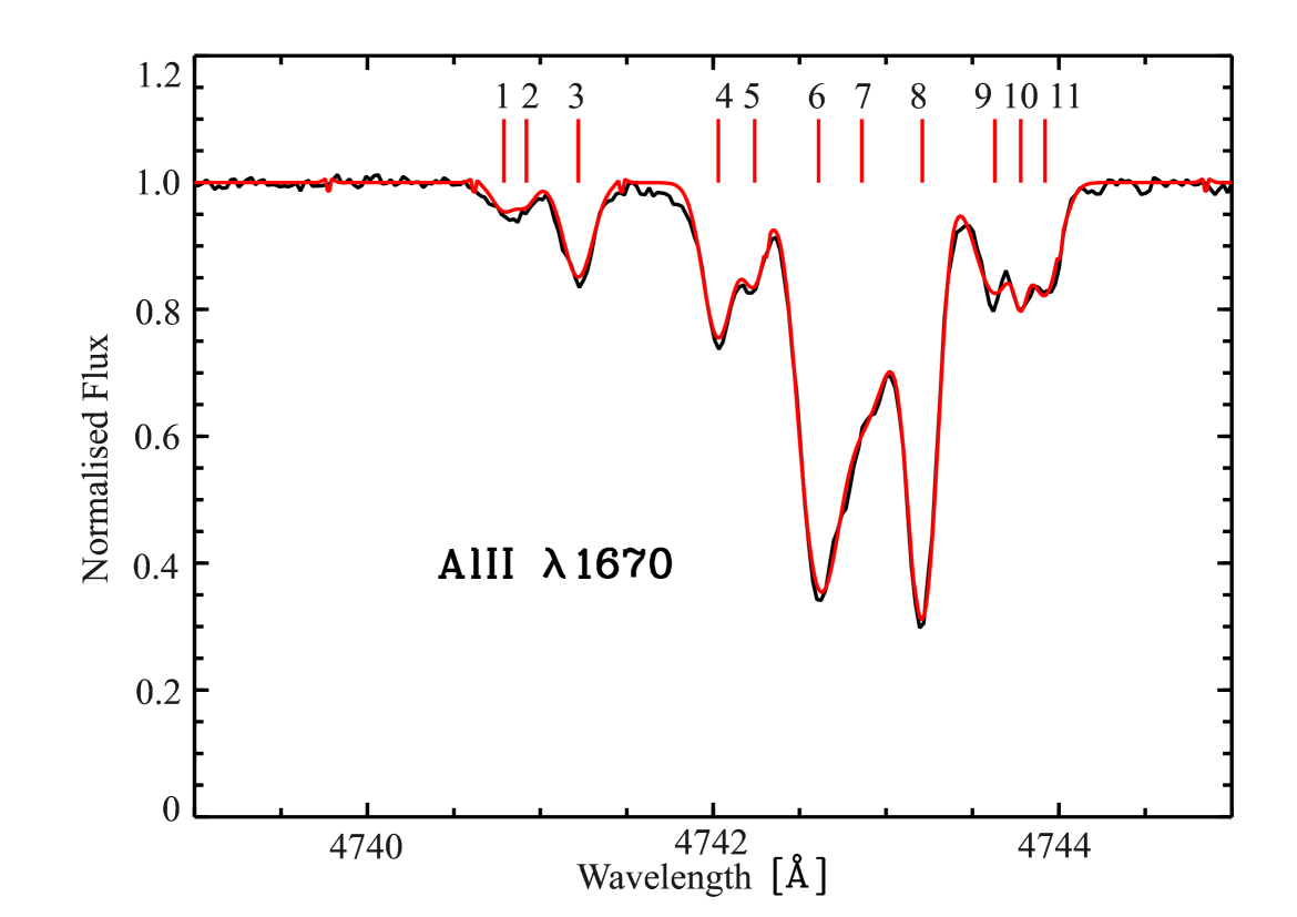
Figure 3: Representative multi-component Voigt profile fit of the Al ii $\lambda 1670.79$ Å absorption feature in the sub-DLA at $z=1.839$. The data and the fit are indicated in black and red. The velocity components used in the fits are indicated by vertical tick marks. Parameters of the fit can be found in Table 1.

We find that a minimum of 11 individual components are required to optimally fit the absorption features evident in the weakly and highly ionised species with satisfying $\chi^{2}$-values. In the following, we number the individual velocity components consecutively, starting with the bluest absorption component. The absorber redshift is set at $z=1.839$. For the weakly ionised species, we identify three dominant velocity components at $-46.3$ km s^-1, $-29.0$ km s^-1, and $-10.2$ km s^-1 (components 6,7, and 8). All subcomponents span a total velocity range of $\Delta v\approx 200$ km s^-1. The relative velocities of all subcomponents are listed in Table 1.

The velocity components of the highly ionised species are less well separated. We identify four dominant velocity components at $-135.6$ km s^-1, $-90.1$ km s^-1, $-43.9$ km s^-1, and $-6.1$ km s^-1 (components 2,3,7, and 9). The relative velocities of all subcomponents are listed in Table 2.

4.2 Neutral and weakly ionised species

In the H i Lyman $\alpha$ absorption, the various velocity subcomponents are superposed in one extended Lyman trough. From a single-component fit of this trough, we obtain a total neutral hydrogen column density of $\log N($H i$)=19.48\pm 0.01$, confirming the earlier results of Dessauges-Zavadsky et al. (2003). The centroid of the Lyman $\alpha$ line lies at $-36.2$ km s^-1, thus between components 6 and 7 of the neutral gas components as traced by O i (see Fig. 2). A component model of the H i absorption, which is in line with the above given value for the total H i column density, is presented in the Appendix. The fit results for the metal species are summarised in Table 1. Unless stated otherwise, the column-density errors given in this paper are the $1\sigma$ fitting errors derived by FITLYMAN. They account for the statistical noise, but do not include uncertainties associated with the tracing of the continuum or systematic uncertainties arising from fixing of the line centres and $b$-values. We decide not to fit the Si iii profiles because of severe saturation. Upper limits for weak or undetected absorption features are listed in Table 2. The comparison to Table 1 shows that for most of the weaker components the fitting procedure did not give reliable results. Some of the fitted components clearly are dominated by noise and the results should be interpreted with caution.

Table 2: Detection limits

Ion A	Detection limit in $\log N$(A)
O i	12.6
N i	12.6
N ii	13.3
Mg i	10.8
Al iii	11.7
S ii	13.2
Fe ii	11.6

4.3 Highly ionised species

Table 3: Results of the fitting procedure for C iv and Si iv

No	$v_{\text{rel}}$ [km s-1]	Ion A	$\log N$(A)	$b$ [km s-1]
1	$-$156.9	C iv	$13.03\pm 0.01$	$13.0\pm 0.3$
		Si iv	$12.66\pm 0.00$	$12.6\pm 0.2$
2	$-$135.7	C iv	$13.31\pm 0.01$	$9.6\pm 0.1$
		Si iv	$12.98\pm 0.00$	$6.9\pm 0.0$
3	$-$92.7	C iv	$13.50\pm 0.02$	$20.6\pm 0.5$
		Si iv	$12.98\pm 0.00$	$20.9\pm 0.3$
4	$-$83.9	C iv	$12.72\pm 0.06$	$6.3\pm 0.4$
		Si iv	$12.77\pm 0.01$	$5.5\pm 0.1$
5	$-$70.9	C iv	$12.71\pm 0.09$	$10.1\pm 1.5$
		Si iv	$12.29\pm 0.01$	$4.7\pm 0.2$
6	$-$53.2	C iv	$12.90\pm 0.07$	$10.0\pm 0.8$
		Si iv	$11.89\pm 0.06$	$6.1\pm 0.7$
7	$-$43.0	C iv	$13.28\pm 0.03$	$14.8\pm 1.0$
		Si iv	$13.30\pm 0.00$	$13.3\pm 0.1$
8	$-$23.2	C iv	$12.49\pm 0.07$	$6.0\pm 0.5$
		Si iv	$12.34\pm 0.02$	$6.0\pm 0.2$
9	$-$6.1	C iv	$13.64\pm 0.01$	$10.1\pm 0.2$
		Si iv	$13.02\pm 0.00$	$11.5\pm 0.1$
10	8.9	C iv	$13.03\pm 0.04$	$9.9\pm 0.4$
		Si iv	$12.12\pm 0.02$	$13.5\pm 0.7$
11	36.2	C iv	$12.57\pm 0.02$	$15.5\pm 0.7$
		Si iv	$12.35\pm 0.01$	$8.0\pm 0.2$

Absorption by highly ionised gas is seen in C iv $\lambda\lambda 1548,1550$, and Si iv $\lambda\lambda 1393,1402$. N v and O vi are located outside the observed wavelength range. We identify 11 absorption components in the high-ion absorption pattern. The results of the fitting procedure are summarised in Table 2. We note that for the high ions the individual velocity components are less well separated than those of the weakly ionised species. This is evident for example in component 8, which seems to be mixed into component 9 in carbon, but in silicon it appears to be mixed into component 7 (see Fig. 4). Therefore, it is likely that the true sub-component structure is not fully resolved.

4.4 Comparison

In Fig. 4, the structure of the absorption lines of the weakly and highly ionised species is compared. For this purpose, the velocity structure of the Mg ii absorption line is used as reference for the weakly ionised species and applied to the C ii and Si ii absorption lines. In a similar way, the velocity structure that results from the simultaneous fit of C iv and Si iv is used as reference for the highly ionised species.

The complex velocity structure in the different ions implies a multi-phase nature of the gas where the ionisation ratios vary among the different components. The gas seems to be more highly ionised in the four bluest subcomponents, whereas in the other subcomponents the weakly ionised species are more dominant. We also note that the line ratios between individual low-ion transitions vary among the different components. Component 5, for example, is apparently stronger in Si ii while it is barely visible in C ii.

Dessauges-Zavadsky et al. (2003) point out that in many sub-DLAs the high-ion transitions commonly show very different absorption profiles compared to low-ion transitions. This trend is also observed in DLAs (Fox et al. 2011, 2007a; Wolfe et al. 2005; Dessauges-Zavadsky et al. 2001; Wolfe & Prochaska 2000; Lu et al. 1996). In contrast to these previous findings, the velocity structure of the highly and weakly ionised species in the system towards QSO B1101$-$26 is rather similar. Most of the velocity components coincide within the uncertainty range for determining the component’s central velocity, which is of the order of 10 km s^-1. This value is calculated from the line centre errors given by FITLYMAN. Kinematic alignment between weakly and highly ionised species has also been found by some other studies (e.g. Lehner et al. 2008). Especially the intermediate ion Al iii has in general the same velocity distribution as the weakly ionised species (Vladilo et al. 2001).

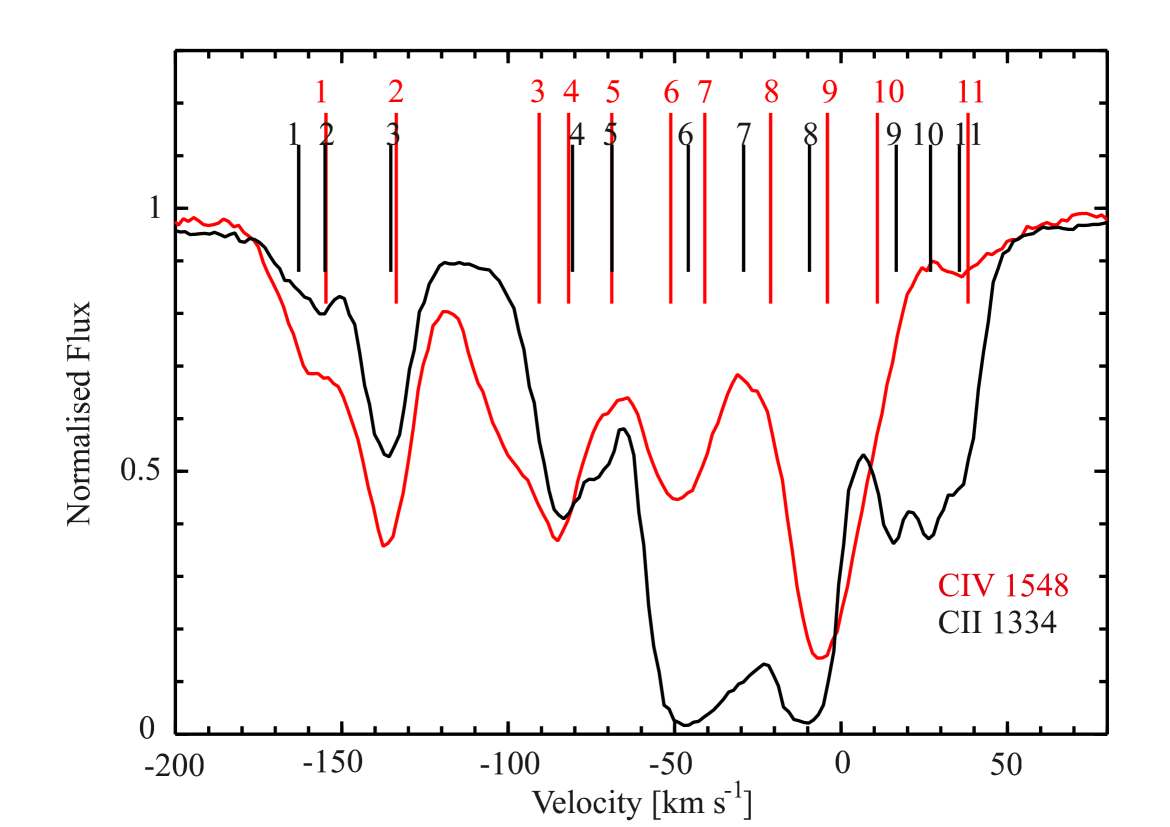
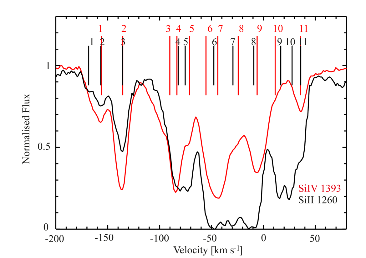
Figure 4: Comparison between the velocity structure of highly and weakly ionised species. Presented are C ii (black) and C iv (red) in the upper panel, and Si ii (black) and Si iv (red) in the lower panel. The vertical tick marks indicate the locations of the line centres of the absorption components.

4.5 Abundances from ion ratios

Throughout this work, abundances are given in the notation [X/Y]$=\log$($N$(X)/$N$(Y))$-\log($X/Y$)_{\odot}$ with solar abundances from Asplund et al. (2009). In this notation, $N$(X) is defined as the sum of the column densities of all ionisation stages of element X. In practice, abundances are usually calculated on the basis of the column density of the dominant ionisation state of element X, because not all ionisation states are available and because it is assumed that the non-dominant ionisation states barely add to the total abundance of X. However, this might not always be true and therefore ionisation corrections will be performed in Sec. 4.6 in order to compensate for significant amounts of X in different ionisation states. In order to distinguish between the real physical abundance ratios of the elements X and Y (or the ionisation corrected abundance) and the abundance ratio simply calculated by the dominant ionisation state, we use the terms [X/Y] and [A/B], respectively, where A is an ionisation state of element X and B is an ionisation state of element Y.

First, we discuss the results for the conventional approach without ionisation corrections. In Table 4 and Fig. 5, the total column densities for the detected species (derived from summing over all absorption components) and the integrated metal abundances are shown. These values have been derived by taking into account the detection limits presented in Table 2, i.e. measured column densities that lie below the formal detection limit have not been considered. The overall metallicity of the absorber, as traced by the $\alpha$-element oxygen, is [O i/H i] $=-1.56\pm 0.01$, and is therefore higher than what has been found by Dessauges-Zavadsky et al. (2003) who estimate [O/H] $=-1.78\pm 0.12$. However, from Fig. 5 and Table 4 O i appears to be underabundant compared to all other available ions. A plausible reason for this apparent underabundance could be an ionisation effect, which will be examined further as part of the Cloudy modelling presented in Sec. 4.6. Dessauges-Zavadsky et al. (2003) also show that S ii appears to be strongly overabundant compared to the other $\alpha$-elements, especially compared to oxygen. We note that the sulphur abundance obtained here deviates substantially (by 0.73 dex) from the sulphur abundance obtained by Dessauges-Zavadsky et al. (2003). However, the dominant contribution to this discrepancy comes from different solar reference abundances used in these two studies (Grevesse & Sauval (1998) vs. Asplund et al. (2009)). There is no obvious origin for such an overabundance, as sulphur and oxygen are jointly produced in the $\alpha$-process and are both non-refractory elements, i.e. they are not influenced by dust-depletion (e.g. Jenkins 2009).

Nevertheless, the ionisation potential of S ii is 23.23 eV, i.e. it is significantly higher than those of O i and H i ($\sim 13.6$ eV for both). This implies that S ii still exists in gas where part of the hydrogen is ionised. By contrast, neutral oxygen is coupled to hydrogen by strong charge-exchange reactions (Osterbrock & Ferland 2006; Field & Steigman 1971). As a consequence, the fraction of oxygen and hydrogen in ionised form should be identical, and if the larger part of the hydrogen is ionised, so will be the oxygen. This aspect will be discussed further in Sec. 4.6.

We note that in our discussion we consider the mean abundances in this system, averaged over several components unless stated otherwise. However, abundance ratios in individual components may significantly deviate from the mean value. This is apparent from Fig. 4. Such behaviour has also been found in other systems, see for example Ledoux et al. (2003) and Richter et al. (2005). In the following, particularly interesting abundance ratios are discussed.

Table 4: Element abundances in the absorption line system at $z=1.839$.

Ion A	$\log N$(A)${}_{\text{tot}}$	Element X	$\log N$(X)⊙	$\log$(A/H i)	[A/H i]	[X/H]2
C ii	$14.73\pm 0.01$	C	$8.43\pm 0.05$	$-4.75\pm 0.01$	$-1.18\pm 0.05$	$-0.96\pm 0.10$
N i	$\leq 12.6$	N	$7.83\pm 0.05$	$\leq-6.88$	$\leq-2.71$	$\ldots$
N ii	$13.44\ldots 14.36^{1}$	N	$7.83\pm 0.05$	$-5.12\ldots-6.04^{1}$	$-0.95\ldots-1.87^{1}$	$\ldots$
O i	$14.60\ldots 14.62^{1}$	O	$8.69\pm 0.05$	$-4.86\ldots-4.88^{1}$	$-1.55\ldots-1.57^{1}$	$-1.78\pm 0.12$
Mg ii	$13.87\pm 0.01$	Mg	$7.60\pm 0.04$	$-5.61\pm 0.01$	$-1.21\pm 0.04$	$-1.01\pm 0.06$
Al ii	$12.85\pm 0.01$	Al	$6.45\pm 0.03$	$-6.63\pm 0.01$	$-1.08\pm 0.03$	$-1.14\pm 0.08$
Al iii	$11.96\ldots 12.77^{1}$	Al	$6.45\pm 0.03$	$-7.52\ldots-6.71^{1}$	$-1.97\ldots-1.16^{1}$	$\ldots$
Si ii	$14.00\pm 0.01$	Si	$7.51\pm 0.03$	$-5.48\pm 0.01$	$-0.99\pm 0.03$	$-1.06\pm 0.05$
S ii	$13.74\ldots 14.29^{1}$	S	$7.12\pm 0.03$	$-5.19\ldots-5.74^{1}$	$-0.31\ldots-0.86^{1}$	$-1.04\pm 0.13$
Fe ii	$13.48\ldots 13.49^{1}$	Fe	$7.50\pm 0.04$	$-5.99\ldots-6.00^{1}$	$-1.49\ldots-1.5^{1}$	$-1.49\pm 0.05$

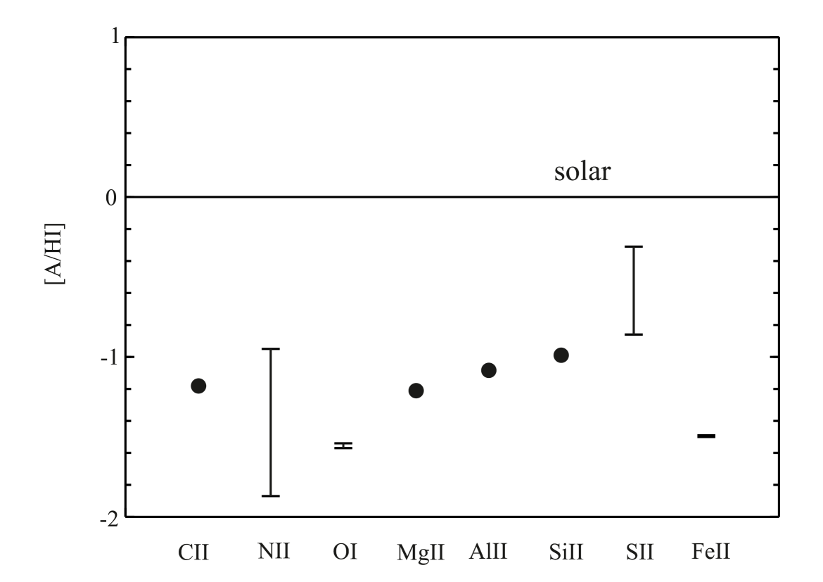
Figure 5: Comparison of element abundances in the absorption line system at $z=1.839$ and solar abundances. Exact values are marked by a filled circle with the error bars being smaller than the symbols itself. Upper and lower limits are marked by horizontal bars.

Nitrogen – The [N/O] ratio provides important information on the chemical evolution and the enrichment history of an absorption system. In the absorber considered here, N i is not detected, but we derive a useful upper limit for N i in the main component (8) (see Table 2). From this, we also obtain an upper limit for the nitrogen-to-oxygen-ratio of [N i/O i]${}_{\text{8}}\leq-0.65$ or $\log$(N i/O i)${}_{\text{8}}\leq-1.55$. This low N i/O i ratio indicates a chemically young system with a delayed production of nitrogen in intermediate-mass stars compared to the quick production of $\alpha$-elements in massive stars. This delay appears to be even more pronounced if one considers the apparent sulphur abundance, yielding [N i/S ii]${}_{\text{8}}\leq-2.26$. Similarly low N/$\alpha$ ratios have also been found in other studies (e.g. Prochaska et al. 2002). For example, Pettini et al. (2008) have found $\log$(N/O$)=-2.53$ to $-1.14$ in their study on metal-poor DLAs. A comparison to their findings about the primary or secondary origin of nitrogen places the absorption system considered here close to the primary plateau. However, ionisation effects can considerably affect the calculation of the nitrogen abundance in sub-DLAs because of the large photoionisation-cross section of neutral nitrogen (Sofia & Jenkins 1998). This aspect will be examined further in Sec. 4.6.

$\alpha$-elements and iron – An overabundance of $\alpha$-elements compared to iron is usually interpreted as the result of the chemical enrichment of protogalactic structures by SN Type II explosions. That is because iron is predominantly produced in SN Type Ia explosions (Matteucci & Greggio 1986; Acharova et al. 2013; Yates et al. 2013) and the progenitors of the SN Type Ia have much longer lifetimes than the progenitors of SNe Type II. A high $\alpha$/Fe ratio is observed in nearly all DLAs (e.g. Prochaska & Wolfe 2002) and also in metal-poor stars of our Galactic Halo, which must have preserved the abundance pattern of the young Milky Way (e.g. Nissen et al. 2004; Suda et al. 2011; Rafelski et al. 2012). In the case of absorption line systems, the conclusion is less straight-forward, because the lack of iron in the gas can also be attributed to dust-depletion. Iron is strongly depleted onto dust grains in the local interstellar medium (Savage & Sembach 1996) and therefore is expected to be underabundant in gas that contains interstellar dust.

In this study, we obtain

$$1.11\leq\log\left(\frac{\text{O\,{\sc i}}}{\text{Fe\,{\sc ii}}}\right) \leq 1.14\text{, or }-0.08\leq\text{[O\,{\sc i}/Fe\,{\sc ii}] }\leq-0.05$$

$$0.51\leq\log\left(\frac{\text{Si\,{\sc ii}}}{\text{Fe\,{\sc ii}}}\right) \leq 0.52\text{, or }0.50\leq\text{[Si\,{\sc ii}/Fe\,{\sc ii}] }\leq 0.51\text{, and}$$

$$0.25\leq\log\left(\frac{\text{S\,{\sc ii}}}{\text{Fe\,{\sc ii}}}\right) \leq 0.81\text{, or }0.63\leq[\text{S\,{\sc ii}/Fe\,{\sc ii}}]\leq 1.19.$$

The values for silicon and sulphur suggest an overabundance of $\alpha$-elements compared to iron, even though silicon is expected to be affected by dust-depletion, too (Savage & Sembach 1996). In contrast, the oxygen-to-iron ratio is significantly lower than other $\alpha$/Fe ratios in sub-DLAs and DLAs and would thus imply a chemically much more evolved system, which seems unlikely in view of the low N i/$\alpha$ ratio and the considered redshift. This discrepancy has its origin in the largely inconsistent $\alpha$-element abundances in the absorber:

$$0.69\leq\text{[S\,{\sc ii}/O\,{\sc i}]} \leq 1.26$$

$$0.13\leq\text{[S\,{\sc ii}/Si\,{\sc ii}] } \leq 0.68$$

$$[\text{Si\,{\sc ii}/O\,{\sc i}}] =0.57\pm 0.07.$$

These ratios do not agree with current nucleosynthetic models in which all $\alpha$-elements are produced at the same time by massive stars, as supported by the observed relative solar abundances of $\alpha$-elements in Galactic halo stars (Nissen et al. 2004). However, similar inconsistencies in the relative abundance of $\alpha$-elements have been found in other high-redshift absorbers, too (e.g. Bonifacio et al. 2001; Prochaska & Wolfe 2002; Fathivavsari et al. 2013).

We note that the large range in the above listed ratios originates in the very weak sulphur absorption, which is below the detection limit in most of the absorption components. A closer look at component 8 reveals a trend possibly caused by ionisation effects that could be the reason for the inconsistent $\alpha$ abundances: [S ii/O i]${}_{\text{8}}=0.98\pm 0.09$, [Si ii/O i]${}_{\text{8}}=0.58\pm 0.07$, [S ii/Si ii]${}_{\text{8}}=0.4\pm 0.07$. In this component, sulphur seems to be the most abundant $\alpha$-element, followed by silicon, and oxygen. This sequence reflects the decreasing order of ionisation potentials of these ions, which are $23.23$ eV, 16.34 eV, and 13.61 eV for S ii, Si ii, and O i, respectively, suggesting that ionisation could be determining the relative strength of the column densities of these ions (see Sec. 4.6).

Carbon – Previous studies of intervening absorbers with achievable carbon measurements have observed an underabundance of carbon compared to $\alpha$-elements (Fechner & Richter 2009; Pettini et al. 2008; Erni et al. 2006; Richter et al. 2005). This is expected from modelling (e.g. Yates et al. 2013) and comparison to metal-poor halo stars (Fabbian et al. 2009; Pettini et al. 2008). Here, we obtain [C ii/Fe ii] $=0.32\pm 0.06$, [C ii/O i] $=0.38\pm 0.07$, $-0.87\pm 0.06\leq$[C ii/S ii] $\leq 0.32\pm 0.06$, [C ii/Si ii] $=-0.19\pm 0.06$, and [C ii/Al ii$]=-0.10\pm 0.06$. Hence, an underabundance of carbon can only be confirmed compared to silicon, sulphur, and aluminium. We note, however, that the carbon absorption line is blended with a weak absorption feature related to an absorption line system at $z=1.268$, for which a transition of Al ii coincides with the carbon line at $z=1.839$.

Odd-even effect – Elements with even atomic numbers are expected to have higher relative abundances because of the strong coupling of pairs of nucleons (Arnett 1971). This effect is probed by the elements Si and Al, with Al being the odd element. Prochaska & Wolfe (2002) have found enhanced Si/Al for the majority of the observed DLA systems, even though the ratios typically are lower than those of metal-poor stars at a similar metallicity (McWilliam et al. 1995). The measured values for our system ([Si ii/Al ii] $=0.09\pm 0.06$) do not indicate a significant odd-even abundance effect.

Dust depletion – It is well known that in Galactic interstellar dust grains the elements iron, aluminium, and magnesium are refractory, silicon and carbon are mildly refractory, and sulphur is essentially non-refractory (Savage & Sembach 1996). Therefore, it is interesting to examine the abundance ratios of refractory and non-refractory elements. We find

$$-0.87\leq \text{ [C\,{\sc ii}/S\,{\sc ii}]}\leq-0.32$$

$$-0.90\leq \text{ [Mg\,{\sc ii}/S\,{\sc ii}]}\leq-0.35$$

$$-0.77\leq \text{ [Al\,{\sc ii}/S\,{\sc ii}]}\leq-0.22$$

$$-0.68\leq \text{ [Si\,{\sc ii}/S\,{\sc ii}]}\leq-0.13$$

$$\text{and}-0.63\leq \text{ [Fe\,{\sc ii}/S\,{\sc ii}]}\leq-1.19.$$

Albeit the large errors, these values are broadly consistent with depletion values for warm Galactic disk gas and halo gas (Savage & Sembach 1996; Welty et al. 1999). Nevertheless, the effects of dust depletion are likely entangled with nucleosynthetic and ionisation effects in this system, as will be discussed below.

4.6 Photoionisation modelling

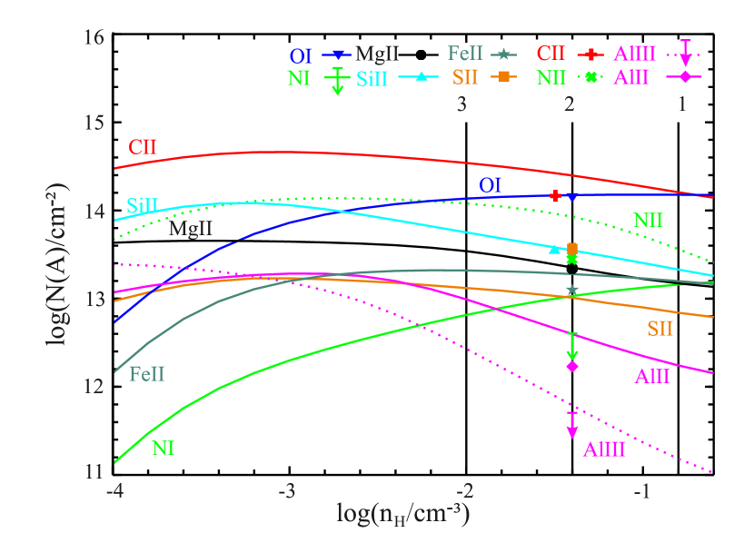
a) Component 8, metallicity of $2.75\%$ solar. The vertical black lines indicate the models 8.1, 8.2, and 8.3 with decreasing hydrogen density.

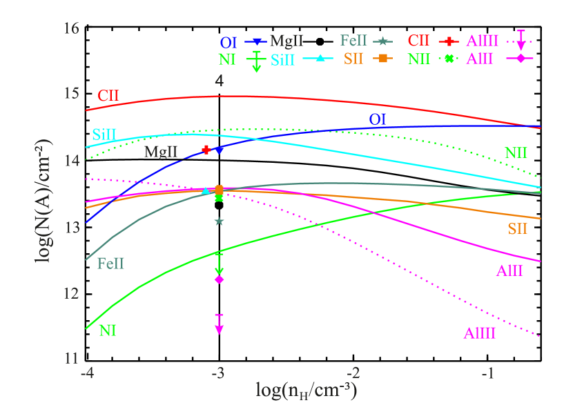
b) Component 8, metallicity of $6\%$ solar. The vertical black line indicates the model 8.4.

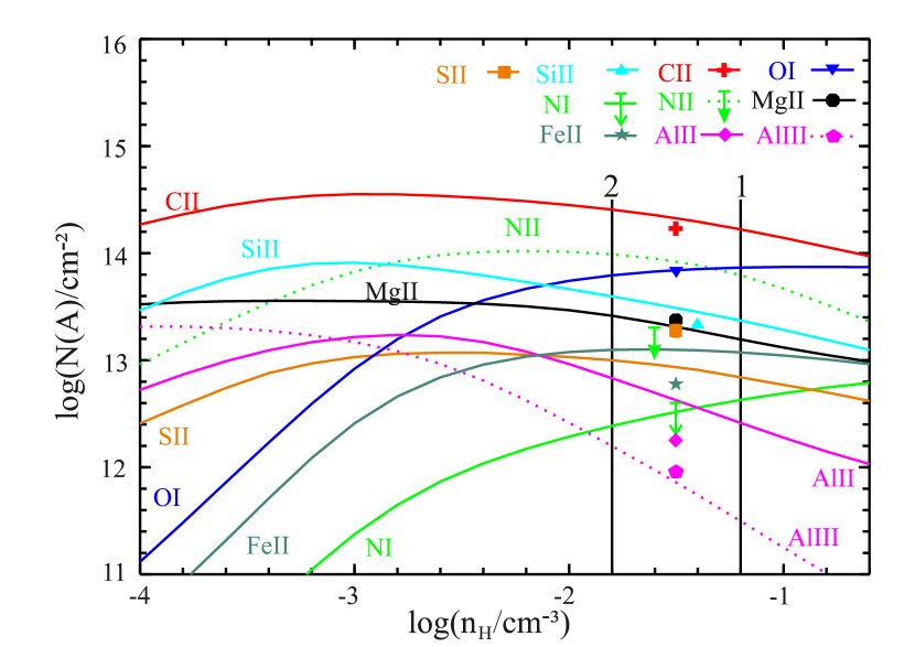
c) component 6, metallicity of 2.75% solar. The vertical black lines indicate the models 6.1, and 6.2 with decreasing hydrogen density.

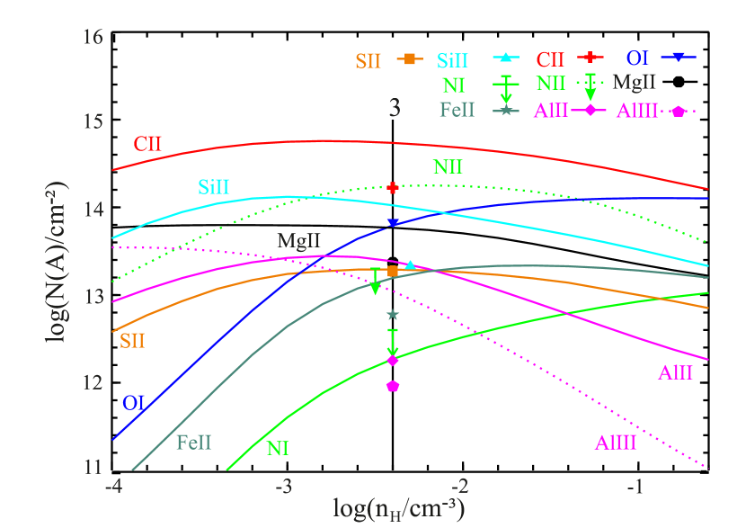
d) component 6, metallicity of 4.7% solar. The vertical black line indicates the model 6.3.

Figure 6: Cloudy models for component 8 (a,b) and 6 (c,d) in the absorption line system at $z=1.839$. The lines represent the Cloudy predictions and the symbols the measured values. The correlation between the symbols and the lines is shown in the legends in the upper right corners. Circles correspond to measured values with the error bars being smaller than the symbol itself except for sulphur. For Al iii and N i an upper limit is given in a) and b). The vertical black lines indicate the hydrogen density of the specific models (see text). Some symbols have a horizontal offset for clarity.

Table 5: Deviations between measured column densities and Cloudy calculations in component 8

Ion A	$\Delta\log N(A)$
	Model 8.1	Model 8.2	Model 8.3	Model 8.4
C ii	0.05	0.24	0.38	0.8
N ii	0.12	0.49	0.64	1.02
O i	0.03	0.02	$-0.02$	0.05
Mg ii	$-0.18$	0	0.19	0.65
Al ii	0.01	0.37	0.76	1.35
Al iii	$\geq-0.52$	$\geq$ 0.09	$\geq$ 0.73	$\geq$ 1.82
Si ii	$-0.22$	0	0.20	0.82
Fe ii	0.10	0.18	0.22	0.44
S ii	$-0.71$	$-0.55$	$-0.43$	$-0.01$
Are the ion ratios reproduced correctly?
(Al ii/Al iii)	no	yes	yes	no
(N i/N ii)	no	yes	yes	yes

Table 6: Deviations between measured column densities and Cloudy calculations in component 6

Ion A	$\Delta\log N(A)$
	Model 6.1	Model 6.2	Model 6.3
C ii	0	0.19	0.52
N ii	0.65	0.85	1.10
O i	0.04	$-0.04$	$-0.04$
Mg ii	$-0.18$	0.05	0.40
Al ii	0.16	0.58	1.13
Al iii	$-0.46$	0.24	1.09
Si ii	0.04	0.27	0.69
Fe ii	0.29	0.31	0.41
S ii	$-0.43$	$-0.27$	0.01
Are the ion ratios reproduced correctly?
(Al ii/Al iii)	no	no	yes
(N i/N ii)	yes	yes	yes

Intervening absorption line systems with large H i column densities beyond a few times $10^{19}$ cm^-2 are usually assumed to be predominantly neutral because of self-shielding of the gas. For such systems, the metallicity in the neutral gas phase is usually determined by comparing the column densities of the dominant (low) ions of heavy elements with the column density of neutral hydrogen, as presented in Sec. 4.5. While the approach is well justified for DLAs (e.g. Wolfe et al. 2005; Vladilo et al. 2001; Viegas 1995) and many sub-DLAs (e.g. Prochaska et al. 2006; Péroux et al. 2006; Dessauges-Zavadsky et al. 2003), ionisation effects may become important for a specific class of sub-DLAs, namely those systems, in which the gas density, and thus the recombination rate, is relatively low, so that the neutral gas fraction falls substantially below unity. These ionisation effects could at least qualitatively explain the unexpected abundances in the previous section. Interestingly, Milutinovic et al. (2010) also report on super-solar metallicities ([S ii/H i]$=+0.36$) in a multi-phase sub-DLA before applying ionisation corrections.

To estimate the influence of ionisation on the determination of metal abundances in our sub-DLA, we carried out photoionisation models using version 10.00 of the Cloudy photoionisation code (Ferland et al. 1998). For this purpose, we assume the incident ionising radiation field to be composed of the cosmic background radiation and a Haardt & Madau (2001) UV background as implemented in Cloudy, both evaluated at the redshift of the absorber. We modelled a plane-parallel slab of gas and varied the hydrogen density $n_{\text{H}}$ between $10^{-5.0}$ and $10^{-0.6}$ cm^-3 in steps of $10^{-0.2}$ cm^-3. The temperature was left as a free parameter. Nevertheless, Cloudy adopted an electron temperature of about $T_{e}\approx 1-2\cdot 10^{4}$ K in every case. Because of the multi-phase nature of the sub-DLA with its different velocity components and a non-uniform gas density among the different components (resulting in a non-uniform ionisation parameter), we set up photoionisation models solely for selected velocity components, for which sufficient spectral line diagnostics are available. We have estimated the H i column density in each component on the basis of the observed column density of O i in the respective component and the assumption that the (O i/H i) ratio is constant throughout the absorber. This assumption is well justified, because of the strong connection of O i and H i by charge-exchange reactions (see also Fig. 9). The simulations were stopped once this H i column density was reached. In our initial modelling approach, we assume a solar chemical abundance pattern taken from Asplund et al. (2009) and scale down the overall metallicity in the gas to 2.75% solar which corresponds to the measured [O i/H i]. Subsequently, we modify the overall metallicity and gas density in order to reproduce the observations, i.e. to best match the column density results obtained by FITLYMAN.

Fig. 6a) and b) show the Cloudy models for component 8. The H i column density for this component is estimated to be $\log N(\text{H\,{\sc i}})=19.02$. We find four models that partly match the observations. The deviations from the measured values are presented in Table 6. In the following, we will discuss their advantages and drawbacks.

Model 8.1 – Model 1 is based on a metallicity of 2.75% solar metallicity, which corresponds to the measured value of [O i/H i], and a hydrogen density of $\log n_{\text{H}}=-0.8$. This model shows the mathematically smallest deviations from the measured values. However, it has some significant drawbacks. O i is slightly overproduced at this density. By contrast, S ii is overabundant compared to the Cloudy calculations. Mg ii is slightly overabundant as well and the ratios of Al ii/ Al iii and N i/ N ii can not be reproduced. Besides, the high hydrogen density seems unlikely for an intergalactic sub-DLA. However, the Al ii/ Al iii ratio might suffer from uncertainties in the recombination rates (Vladilo et al. 2001).

Model 8.2 – This model assumes again a metallicity of 2.75% solar but a hydrogen density of $\log n_{\text{H}}=-1.4$. It produces the measured column densities of O i, Si ii, and Mg ii correctly, i.e. all available $\alpha$-elements except for sulphur which is again overabundant compared to the model. However, the Cloudy model predicts too much C ii, Fe ii, aluminium, and nitrogen. An underabundance of Fe ii and nitrogen in this system could be due to nucleosynthetic effects. An underabundance of carbon is often observed in DLAs (see Sec. 4.5). Aluminium, on the other hand, might suffer from uncertainties in the shape of the ionising spectrum or be subject to an intrinsic underabundance compared to a solar abundance pattern (Crighton et al. 2013; Rolleston et al. 2003). Despite the underabundance, the ratios of Al ii/ Al iii and N i/ N ii are modelled correctly.

Model 8.3 – This model is based on a metallicity of 2.75% solar and a hydrogen density of $\log n_{\text{H}}=-2.0$. It indicates the low density limit of the range where the Al ii/ Al iii and N i/ N ii ratios match the observations, whereas the high density limit is indicated by Model 8.2. The O i column density is well reproduced. Too little S ii is produced. All other column densities are overproduced compared to their measured values. These underabundances can qualitatively be explained by nucleosynthesis and dust depletion. The ratios of Al ii/ Al iii and N i/ N ii are modelled correctly.

Model 8.4 – This model is based on a metallicity of 6% solar and a hydrogen density of $\log n_{\text{H}}=-3.0$. The metallicity in this model does not correspond to the measured value of [O i/H i], but it produces the column densities of O i and S ii correctly. However, it overproduces all of the other column densities. An underabundance can again be qualitatively explained by nucleosynthesis and dust depletion. The N i/ N ii ratio is reproduced correctly, but the Al ii/ Al iii ratio is not. Besides, a hydrogen density of $\log n_{\text{H}}=-3.0$ seems rather low for a sub-DLA system. Such a very low gas density together with the total gas column density would imply a linear size of this absorption component of several dozen kpc, which is implausible.

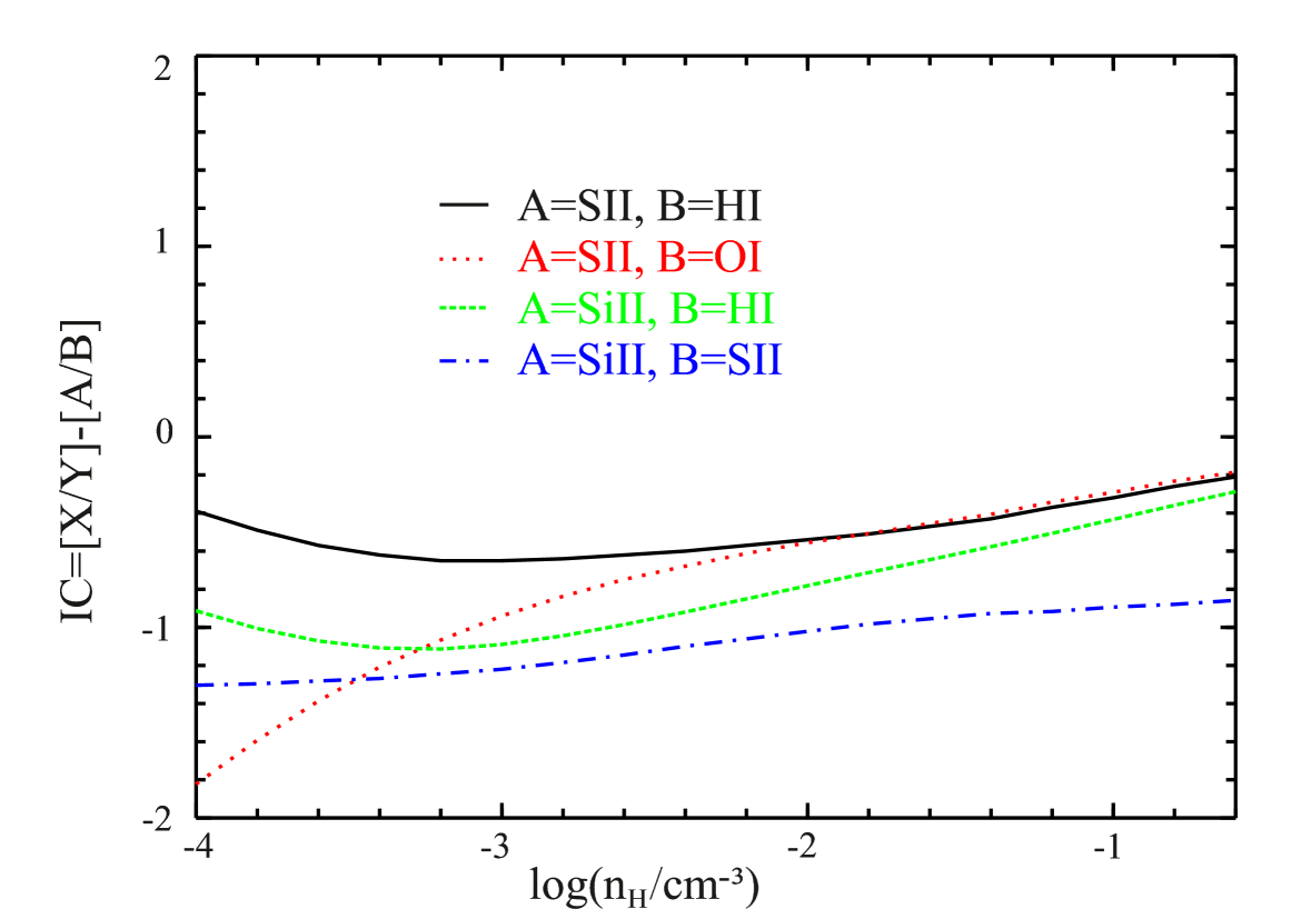
Figure 7: Ionisation correction factors for some elemental column densities in component 8 derived by Cloudy. The model is based on cosmic microwave background radiation and a Haardt & Madau (2001) UV background, relative solar chemical abundances, and a metallicity of 2.75% solar. The correction factors are significant, but they cannot explain the full discrepancy between sulphur and the other elements measured.

Fig. 7 presents the correction factors that can be derived by the Cloudy models. The correction factors show the deviation between the real intrinsic abundances in the gas and the abundances indicated by the dominant ionisation stages:

IC= [X/Y] - [A/B],

i.e. they give an estimate of the systematic bias that occurs when ionisation effects are neglected. These corrections are already included in Fig. 6, because Cloudy considers ionisation effects when calculating the column densities. Therefore, the discrepancy between the expected and the measured values cannot be explained by ionisation even though the ionisation corrections for S ii and Si ii are significant. In order to estimate the uncertainties caused by the choice of the ionising spectrum, we have performed more Cloudy calculations for alternative ionising backgrounds. They can be found in the Appendix. None of them can reproduce the observed column density pattern. We note that the significant correction factors found here are in contradiction to previous studies of higher column density DLAs, which find that corrections are generally small or even below measurement errors (e.g. Vladilo et al. 2001).

As none of the models can fully explain the observed abundance pattern, we are forced to conclude that either there is a large intrinsic overabundance of sulphur in this absorption component, or the absorption feature that falls on the S ii $\lambda 1259$ line at $z=1.839$ is not due to sulphur, but to a blend from another line, or there is unresolved substructure and multi-phase gas in this absorption component, so the Cloudy model cannot correctly reproduce the column-density ratios of the different ions.

Fig. 6c) and d) show similar Cloudy models for component 6. This component is especially interesting, because we can give an exact value for Al iii and not just an upper limit. The H i column density in this component is estimated to be $\log N$(H i) $=18.7$, based on the (O i/H i) ratio. We find three models that partly match the observations. The deviations from the measured values are presented in Table 6.

Model 6.1 – This model is based on 2.75% solar metallicity and a hydrogen density of $\log n_{\text{H}}=-1.2$. It indicates the high density limit of the range where the O i column density matches the observations whereas Model 6.2 indicates the low density limit. Model 1 also reproduces the C ii and Si ii column density, but it underproduces magnesium and sulphur and overproduces iron. The N i/ N ii ratio agrees with the upper limits, but the Al ii/ Al iii is not predicted correctly.

Model 6.2 – This model is based on 2.75% solar metallicity and a hydrogen density of $\log n_{\text{H}}=-1.8$. It correctly reproduces the O i and Mg ii column density. It does not produce enough S ii column density. The rest of the ionic column densities are overproduced. Again, the N i/ N ii ratio agrees with the upper limits, but the Al ii/ Al iii is not predicted correctly.

Model 6.3 – This model is based on 4.7% solar metallicity and a hydrogen density of $\log n_{\text{H}}=-2.4$. It correctly reproduces the O i and S ii column density. All other ions are overproduced which could be caused by nucleosynthetic or dust depletion effects. The Al ii/ Al iii and N i/ N ii ratios are reproduced correctly despite the underabundance of aluminium and nitrogen.

Most interestingly, Fig. 6d) indicates that sulphur is not overabundant in this sub-component if we assume an influence of nucleosynthesis and dust depletion and a metallicity that does not agree with the measured [O i/H i].

We note that, in previous studies, Al iii often shows a different behaviour than the weakly ionised species. Vladilo et al. (2001) have suggested that Al iii might originate in a region different from the one where the weakly ionised species arise. In that case, the Al ii/Al iii ratio would stand for the relative contribution of these separate regions rather than the ionisation state of a single region. On that account, a mismatching Al ii/Al iii ratio does not necessarily have to be a criterion for exclusion for a model.

4.7 S ii absorption

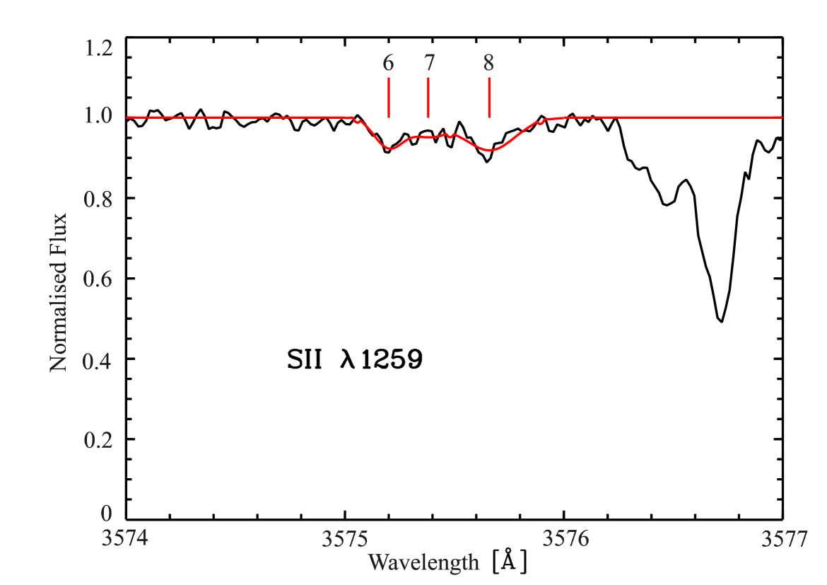
Figure 8: Multi-component Voigt profile fit of the absorption line of S ii $\lambda$1259 in the sub-DLA at $z=1.839$. The data are black and the fit is red. The velocity components used in the fits are indicated by vertical tick marks. Only the main components have been fitted and they are numbered according to the velocity components of the other weakly ionised species. Parameters of the fit can be found in Table 1.

Accurate measurements of sulphur in interstellar and intergalactic gas are particularly desirable, because S is a tracer for the $\alpha$-abundance in the gas and this element is undepleted in dust. For example, Nissen et al. (2004) list sulphur measurements in DLAs from redshift $\approx 1.8-3.4$, which they culled from the literature. Som et al. (2013) measure (among other things) sulphur abundances in sub-DLA systems with redshifts between $\approx 1.7-2.3$. Sparre et al. (2014) show measurements of sulphur and other metals in QSO and gamma-ray burst spectra up to $z\approx 6$, also culled from the literature. Centurión et al. (2000) report on sulphur measurements in DLAs at $z\geq 2$. On the other side of the redshift scale, Richter et al. (2013) and Fox et al. (2013) have studied S ii abundances in the Magellanic Stream.

High metallicity in general is observed sometimes in intervening absorption line systems. Nissen et al. (2004) report on some similarly high sulphur abundances in DLAs. Noterdaeme et al. (2010), Péroux et al. (2006), and Prochaska et al. (2006) even find super-solar metallicities in sub-DLAs and Super Lyman Limit Systems, respectively ([S/H]$=0.15\pm 0.13$, [Zn/H]$=0.61$, and [S/H]$=0.79$, respectively). Considering the measured [O i/H i], a generally high metallicity does not seem to be the case here. However, in the system presented here, the sulphur abundance appears to be much higher than for the other $\alpha$-elements (see Table 4). Interestingly, even though Péroux et al. (2006) do not measure the sulphur abundance in their system, they find evidence of a non-solar abundance pattern as well.

Another point to consider is the [O i/Fe ii] ratio that does not show the expected $\alpha$-enhancement (see Sec. 4.5). Sulphur, on the other hand, is overabundant compared to iron, but we note that Nissen et al. (2004) also do not find evidence of $\alpha$-enhancement in their collection of DLAs from the literature. This can be interpreted as evidence for low and intermittent rates of star formation over the history of the observed absorption systems (Calura et al. 2003). In this scenario, the overall metallicity grows slowly with time and the abundance of iron-peak elements can approach the abundance of $\alpha$-elements in periods without extensive star formation. Such a trend can be observed locally in dwarf irregular and dwarf spheroidal galaxies, whose stars also do not show $\alpha$-enhancement at low metallicities (e.g. Shetrone et al. 2003; Tolstoy et al. 2003).

As we have discussed in Sec. 4.6, photoionisation cannot be the origin of the apparent overabundance of sulphur in the absorber at $z=1.839$, but the Cloudy models suggest that the origin for this discrepancy lies in the 8th absorption component, where the S ii $\lambda 1259$ absorption is particularly strong. This is an unexpected trend that clearly needs further exploration. For this reason, we will discuss in the following different scenarios that may explain the apparently high sulphur abundance in this system.

Fig. 8 shows a zoom-in of the absorption profile of S ii $\lambda 1259$ together with a part of the Si ii $\lambda 1260$ absorption feature. Significant absorption in the $\lambda 1259$ line is evident only for the main components 6, 7, and 8. We note that S ii $\lambda 1253$ is unfortunately blended by a Ly $\alpha$ interloper, while possible absorption in the weak S ii $\lambda 1250$ transition is obviously below the detection limit. While the S/N in the spectral region near the S ii $\lambda 1259$ line is mildly lower than in other regions of the spectrum (see Fig.  2), the absorption feature is clearly detected and cannot be caused by a noise feature.

In principle, there are three possible explanations for the derived overabundance:

1. The detection of sulphur is false positive. – In the first place, it is stunning that sulphur turns out to be overabundant compared to all other detected elements (see Fig. 5). This overabundance cannot be explained by current nucleosynthesis theories, as sulphur is supposedly produced together with the other $\alpha$-elements. As oxygen is also not depleted onto dust grains, sulphur and oxygen should have the same gas-phase abundances. Moreover, the obtained abundance range $-0.86\leq\text{[S\,{\sc ii}/H\,{\sc i}]}\leq-0.31$ indicates a metallicity of $\approx 14-49$% solar, which is far above what is expected for protogalactic systems at this high redshift and is also inconsistent with the oxygen metallicity. These aspects put the actual detection of sulphur in our absorber into question, possibly implying that the absorption feature shown in Fig. 8 is not due to S ii $\lambda 1259$ absorption at $z=1.839$, but is caused by another absorption line at a different redshift. There is, however, no other prominent absorption system in the spectrum that we are aware of that could be the origin for this absorption feature near 3575 Å. Theoretically, the absorption could also be caused by a very blue component of the Si ii $\lambda 1260$ line, but this is highly unlikely because no other line indicates clues for any additional absorption components at the considered relative velocity. In addition, the position and relative strength of the absorption components in the absorption feature shown in Fig. 8 almost perfectly match the expected component structure of S ii $\lambda 1259$ at $z=1.839$. The probability that a random absorption feature from another intervening absorber reproduces by chance the shape of the expected S ii absorption at $z=1.839$ is extremely small. Thus, we are forced to conclude that any interpretation of the absorption feature at 3575 Å other than being S ii $\lambda 1259$ at $z=1.839$ is very unlikely. In addition, systematic errors arising from the uncertainties in the atomic data are not expected to play a significant role (Kisielius et al. 2014).

2. Sulphur is overabundant in this system due to mixing, non-equilibrium, or nucleosynthetic effects. – A sightline passing through intergalactic or galactic gaseous structures only probes a pencil beam, and thus it is not guaranteed that the conditions along this sightline are representative for the whole structure. Peculiar element abundances could arise from gas underlying dynamic processes or gas that is not well mixed. Evidence for this is given by a comparison of the absorption profiles of different elements (see Sec. 4.4). Abundance ratios that cannot be explained by current nucleosynthetic theories have also been found by other groups, e.g. by Fathivavsari et al. (2013), who find sulphur being overabundant compared to oxygen in a sub-DLA, by Bonifacio et al. (2001), who find sulphur being overabundant compared to oxygen, silicon, and iron even though [S/H]$=-1.04$ in the considered DLA, and by Lehner et al. (2008). On the other hand, super-solar [S/Si] and [S/Fe] ratios could be caused by dust-depletion. Another possible explanation for high sulphur abundances could be hypernovae with exploding He-cores, which, according to Nakamura et al. (2001), overproduce sulphur. However, this theory has been disputed by Nissen et al. (2004) who show that the general behaviour of sulphur is in good agreement with near-instantaneous production of $\alpha$-elements by Type II supernovae. Furthermore, the drawback of the assumption that sulphur is overabundant due to one of the above effects is that it provides no explanation for the apparent underabundance of oxygen which leads to a lack of $\alpha$-enhancement. By contrast, the sulphur abundance supports the super-solar [Si ii/Fe ii] ratio.

3. The apparent high sulphur abundance is caused by ionisation effects. – The Cloudy models presented here are not unique. Different ionisation conditions can result in different abundance ratios. For example, an incident radiation field following a power law can produce the observed [S ii/O i] ratio. However, this model cannot predict the Al ii/Al iii ratio correctly. Evidence for the sulphur abundance being correct might be the observed [$\alpha$/Fe ii] ratios that only show the expected $\alpha$-enhancement for Si ii and S ii, but not for O i. Furthermore, previous studies of Richter et al. (2005) and Erni et al. (2006) have found an underabundance of carbon in the considered (sub-)DLAs. In the system considered here, we can report an underabundance of carbon in relation to S, Si and Al, but carbon is overabundant compared to oxygen and iron. On the other hand, the detected C ii absorption line is likely blended by a weak absorption feature of Al ii at $z=1.268$. Another argument that supports the sulphur abundance found here, is an estimation for the expected sulphur abundance in DLAs taken from Prochaska & Wolfe (1999): They argue that an abundance pattern being consistent with SN Type II enrichment and dust-depletion requires [S/Fe]$>0.6$. This is because, on the one hand, sulphur as $\alpha$-element is observed to be overabundant relative to Fe in metal-poor halo stars by $\approx 0.3-0.5$ dex and, on the other hand, [Zn/Fe] values resulting from dust-depletion suggest [S/Fe]$>0.3$ dex on the basis of depletion alone. Even though Prochaska & Wolfe (1999) find values that are inconsistent with this estimation, the expected [S/Fe]$>0.6$ is consistent with our results, but other ion ratios (see above) remain inconsistent.

As none of the above three scenarios can explain individually the unusually high abundance of S ii in the absorber, we suggest that the observed abundance pattern in this system reflects a particular local environment in the absorbing gas structure where the (combined) effects of a multi-phase nature of the gas (see also Fumagalli 2014), unusual intrinsic abundances, dust depletion, and/or unresolved sub-component structure are relevant. Neutral gas coexisiting with ionised gas can result in peculiar abundance ratios and Cloudy is unable to model multi-phase systems (see Milutinovic et al. 2010; Lehner et al. 2008; Fox et al. 2007b). Besides, a multi-phase gas structure is motivated by the evidently strong interlacing of the absorption components of highly and weakly ionised species (see Fig. 4). This point of view is also motivated by previous studies of our Galactic halo, e.g. Howk et al. (2006) who argue that comparing the column densities of the dominant ionisation stages of metals to the column density of neutral hydrogen along a line of sight will result in apparently too high metal abundances.

5 Relevance to other studies

The sub-DLA system at $z=1.839$ is an excellent example for our lack of understanding of the physical and chemical conditions in intervening absorption line systems. Our detailed analysis reveals that, despite of the excellent data quality (or rather because of), the derived abundances for the two $\alpha$-elements O and S cannot be explained by a standard SN Type II enrichment pattern, even if photoionisation effects are included. In the light of the very high resolution used here, discrepancies arise that challenge the results of lower-resolution studies on intergalactic absorption line systems. Especially, the summing up of metal abundances and the averaging of temperatures and densities over these absorbing structures – an often used approach for the interpretation of multi-component absorbers – seems questionable, taking into account the substantial differences that we find between single velocity components of the same absorber. In contrast to current theories, the abundance pattern in this system is neither completely in line with a SN Type II enrichment pattern, nor with an ISM-like dust-depletion pattern, nor with a combination of the two if we take into consideration the puzzling S ii absorption. On the other hand, ignoring the S ii absorption leaves us with a striking underabundance of oxygen, evident from Fig. 5. This would result in a lack of $\alpha$-enhancement, which would be commonly expected for intervening absorption systems, and requires strong depletion values to fit the Cloudy models, which seems unlikely.

As has been pointed out in Sec. 4.7, peculiar sulphur abundances have also been found by Bonifacio et al. (2001), and Fathivavsari et al. (2013) have derived abundances of $\alpha$-elements not being in line with each other in sub-DLA systems. Other detailed studies of multi-component absorbers at high redshift provide further evidence of significant discrepancies between a standard SN Type II enrichment pattern and measured gas-phase abundances in individual absorption components. For instance, Richter et al. (2005) have studied a very complex sub-DLA at $z=2.187$ towards the quasar HE 0001$-$2340, finding substantial overabundance of several heavy elements (including phosphorus and aluminum) in two absorption components, even after applying an ionisation correction. These authors conclude that the gas belonging to these components is possibly enriched locally by the supernova ejecta from one or more massive stellar clusters. The lack of mixing of heavy elements in the interstellar and circumgalactic gas of galactic and protogalactic structures at high redshift is not unexpected, however, because the assembly and evolution of galaxies in that epoch is boosting and coming along with intense (but spatially irregular) star-formation episodes on time scales that can be shorter than the mixing-time scales of metals in the gas. In addition to the chemical enrichment, the local ionisation conditions may also vary dramatically in the presence of star-forming regions and may strongly deviate from a standard UV background model as commonly used to model intervening absorbers at high $z$. In the light of these arguments, the peculiar abundances found by us in the sub-DLA at $z=1.839$ towards the quasar B1101$-$26 could be yet another example for a rather local phenomenon in a protogalactic structure related to star-formation activity (see e.g. Crighton et al. 2013; Prochter et al. 2010; D’Odorico & Petitjean 2001).

In general, an inhomogeneous distribution of metals (including dust) and irregular ionisation conditions in sub-DLAs and DLAs might be major problems for the interpretation of metal abundances in these absorbers. Metal abundances derived from a single sightline may not be representative at all for the host galaxy of the absorber and averaging metal abundances over several velocity components will lead to meaningless results if the metal distribution is patchy within the absorber. It is also important to note that such metal-mixing issues are not restricted to high redshifts. One particular prominent example for an inhomogeneous distribution of heavy elements in a sub-DLA at $z=0$ is the Magellanic Stream (MS), a massive tidal gas structure located at $\sim 50-60$ kpc distance from the Milky Way that has been ripped off the Magellanic Clouds $\sim 1-2$ Gyr (Wannier & Wrixon 1972; Gardiner & Noguchi 1996). In a recent study, Richter et al. (2013) and Fox et al. (2013) have found that the metallicity in the MS varies by a factor of 5 between the main body of the Stream ($0.1$ solar) and the region that is close to the Magellanic Clouds ($0.5$ solar). For the MS sightline towards Fairall 9 Richter et al. (2013) used sulphur as a proxy for the $\alpha$-abundance in the gas. Interestingly, they determine a sulphur abundance in the MS towards Fairall 9 that is higher than the present-day sulphur abundance in the Magellanic Clouds (their Fig. 9), suggesting a local $\alpha$ (sulphur) enrichment by massive stars before the gas was separated from the Magellanic Clouds and incorporated into the MS. The high sulphur abundance is an interesting similarity between the high-redshift sub-DLA towards the quasar B1101$-$26 and a very local tidal gas stream, indicating that our understanding of the metal-abundance pattern in gaseous structures that have been enriched locally by massive stars is yet incomplete.

We conclude that the aspect of abundance anomalies in sub-DLAs and DLAs at low and high redshift, such as presented here, needs further investigation to better understand enrichment and mixing processes in gas at high redshift and to constrain the effect of local phenomena for the interpretation of metal absorption in intervening absorbers.

6 Summary and conclusions

We have performed a detailed analysis of the sub-DLA at $z=1.839$ towards the quasar B1101$-$26 using VLT/UVES spectral data with very high spectral resolution ($R\sim 75,000$) and a very high S/N of $>100$. Our results can be summarised as follows:

• We identify 11 absorption subcomponents in neutral, weakly, and highly ionised species. Detected species include C ii, C iv, N ii, O i, Mg i, Mg ii, Al ii, Al iii, Si ii, Si iii, Si iv, Fe ii, and possibly S ii. These components span a restframe velocity range of $\approx 200$ km s^-1. The fit of the Lyman $\alpha$ absorption line yields a column density of neutral hydrogen of $\log N(\text{H\,{\sc i}})=19.48\pm 0.01$.

• The metallicity of this system, as traced by [O i/H i], is $-1.56\pm 0.01$. However, a peculiar abundance ratio between oxygen and sulphur is found with $0.69\leq$ [S ii/O i] $\leq 1.26$. Concludingly, sulphur indicates a much higher metallicity than oxygen.

• For the nitrogen-to-oxygen ratio, we derive an upper limit of [N i/O i] $\leq-0.65$, which suggests that the absorber is chemically young. This conclusion is also supported by a supersolar $\alpha$/Fe ratio of [Si ii/Fe ii] $\approx 0.5$. However, this ratio might be affected by dust-depletion.

• The abundance pattern in this system is not consistent with SN Type II enrichment combined with the effects of dust-depletion. The low oxygen-to-iron ratio ($-0.08\leq\text{[O\,{\sc i}/Fe\,{\sc ii}]}\leq-0.05$) implies a lack of $\alpha$-enhancement, the observed $\alpha$-elements do not follow each other, and there is no obvious reason for sulphur being overabundant relative to oxygen.

• Comparing our study with previous studies on this absorption line system, it is evident that we could resolve the absorption lines of the weakly and the highly ionised species into more velocity subcomponents because of the higher resolution of the new UVES data. The detection of N ii and the derivation of safe upper and lower limits for the weak absorption features provide additional information on the chemical composition of the gas.

• We have calculated detailed photoionisation models using Cloudy. They yield a metallicity between 2.7% and 6.0% solar and a hydrogen density between $10^{-0.8}$ and $10^{-3.0}$ cm^-3. The predicted column densities also suggest a depletion of the refractory elements including silicon and an underabundance of nitrogen. Furthermore, the Cloudy models indicate that the bigger part of the hydrogen gas in this system is ionised and only a small fraction is in the neutral gas phase. The Cloudy models cannot, however, explain the unusually high [S ii/O i] ratio in this system.

• We discuss possible origins for the peculiar overabundance of sulphur in the absorber. We suggest that the high [S ii/O i] ratio is caused by the combination of several relevant effects, such as specific ionisation conditions in multi-phase gas, unusual relative abundances of heavy elements, and dust depletion. The sightline possibly passes a local gas environment that is not well mixed and that might be influenced by star-formation activity in the sub-DLA host galaxy. We discuss the implications of our findings for the interpretation of $\alpha$-element abundances in metal absorbers at high redshift.

Appendix A Modelling of Lyman $\alpha$ absorption

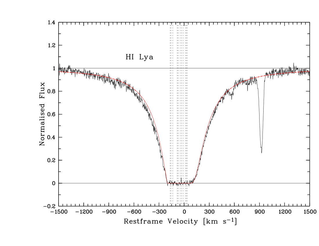
Figure 9: Remodelling of the hydrogen Lyman $\alpha$ absorption line in this absorption system. The absorption line profile is overlayed by the model (red) which is based on the measured O i column density and the assumption that [O i/H i]$=-1.56$ in every component. The vertical, dotted lines indicate the velocity components of the weakly ionised metal species. The shape of the absorption line is reproduced although the outer, weaker components do not give strong constraints on $N$(H i).

Appendix B Additional Cloudy models

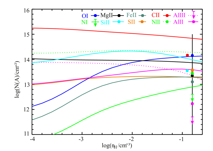
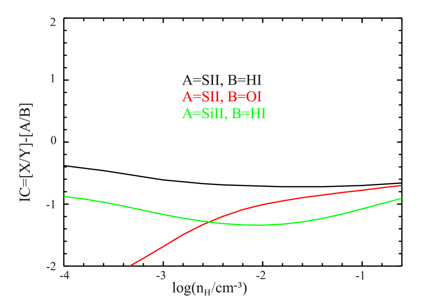
a) Cloudy Model for component 8 based on the radiation field of an O star. The spectral energy distribution used (Tlusty) has been described in Lanz & Hubeny (2003) and has been prepared by Peter van Hoof for the implementation in Cloudy. The metallicity has been set to 2.75% solar and the integrated mean intensity of the radiation field at the illuminated face of the cloud has been set to $10^{-2.8}$ erg cm^-2 s^-1. b) Ionisation correction factors on the basis of a Cloudy model assuming the stellar radiation field of an O star and a metallicity of 2.75% solar like in a).

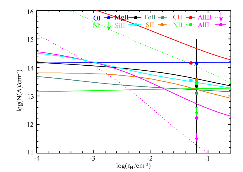
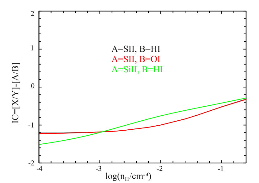
c) Cloudy Model for component 8 based on the Galactic interstellar radiation field scaled by the factor 0.1. The metallicity was set to 2.75% solar. d) Ionisation correction factors on the basis of a Cloudy model assuming a Galactic interstellar radiation field like in c) and a metallicity of 2.75% solar.

Figure 10: (c) Cloudy test model for component 8 in the absorption line system at $z=1.839$. The lines represent the Cloudy predictions and the symbols the measured values. The correlation between the symbols and the lines is shown in the legends in the upper right corners. Circles correspond to measured values with the error bars being smaller than the symbol itself except for sulphur. For Al iii and N i upper limits are given. The vertical black lines indicate the hydrogen density of our favourite models. The symbols sometimes have an offset for clarity. (d) Ionisation correction factors derived by Cloudy based on model c). It is evident that the correction factors are significant, but these (unrealistic) test models, that have been set up to explore the Cloudy parameter range, cannot reproduce the observed abundance pattern, as expected.