A primal-dual mimetic finite element scheme for the rotating shallow water equations on polygonal spherical meshes

Abstract

A new numerical method is presented for solving the rotating shallow water equations on a rotating sphere using quasi-uniform polygonal meshes. The method uses special families of finite element function spaces to mimic key mathematical properties of the continuous equations and thereby capture several desirable physical properties related to balance and conservation. The method relies on two novel features. The first is the use of compound finite elements to provide suitable finite element spaces on general polygonal meshes. The second is the use of dual finite element spaces on the dual of the original mesh, along with suitably defined discrete Hodge star operators to map between the primal and dual meshes, enabling the use of a finite volume scheme on the dual mesh to compute potential vorticity fluxes. The resulting method has the same mimetic properties as a finite volume method presented previously, but is more accurate on a number of standard test cases.

1 Introduction

In order to exploit the new generation of massively parallel supercomputers that are becoming available, weather and climate models will require good parallel scalability. This requirement has driven the development of numerical methods that do not depend on the orthogonal coordinate system and quadrilateral structure of the longitude-latitude grid, whose polar resolution clustering is predicted to lead to a scalability bottleneck. A significant challenge is to obtain good scalability without sacrificing accuracy; in particular conservation, balance, and wave propagation are important for accurate modelling of the atmosphere (Staniforth and Thuburn, 2012).

Building on earlier work (Ringler et al., 2010; Thuburn and Cotter, 2012), Thuburn et al. (2014) presented a finite volume scheme for the shallow water equations on polygonal meshes. They start from the continuous shallow water equations in the so-called vector invariant form:

$$\phi_{t}+\nabla\cdot\mathbf{f} = 0,$$ (1)

$$\mathbf{u}_{t}+\mathbf{q}^{\perp}+\nabla(\phi_{\mathrm{T}}+k) = 0,$$ (2)

where $\phi$, the geopotential, is equal to the fluid depth times the gravitational acceleration, $\phi_{\mathrm{T}}=\phi+\phi_{\mathrm{orog}}$ is the total geopotential at the fluid’s upper surface including the contribution from orography, $\mathbf{u}$ is the velocity, $\mathbf{f}=\mathbf{u}\phi$ is the mass flux, and $k=|\mathbf{u}|^{2}/2$. The $\perp$ symbol is defined by $\mathbf{u}^{\perp}=\mathbf{k}\times\mathbf{u}$ where $\mathbf{k}$ is the unit vertical vector. Finally, $\pi=\zeta/\phi$ is the potential vorticity (PV), where $\zeta=f+\xi$ is the absolute vorticity, with $f$ the Coriolis parameter and $\xi=\mathbf{k}\cdot\nabla\times\mathbf{u}$ the relative vorticity, and $\mathbf{q}=\mathbf{f}\pi$ is the PV flux. By the use of a C-grid placement of prognostic variables, and by ensuring that the numerical method mimics key mathematical properties of the continuous governing equations (hence the term ‘mimetic’), the scheme was designed to have good conservation and balance properties. These good properties were verified in numerical tests on hexagonal and cubed sphere spherical meshes. However, their scheme has a number of drawbacks. Most seriously, the Coriolis operator, whose discrete form is essential to obtaining good geostrophic balance, is numerically inconsistent and fails to converge in the $L_{\infty}$ norm (Weller, 2014; Thuburn et al., 2014). Also, although the gradient and divergence operators are consistent, their combination to form the discrete Laplacian operator also fails to converge in the $L_{\infty}$ norm in some cases. These inaccuracies are clearly visible in idealized convergence tests, and give rise to marked ‘grid imprinting’ for initially symmetrical flows. Although they are less conspicuous in more complex flows, they are clearly undesirable.

Cotter and Shipton (2012) (see also McRae and Cotter, 2014; Cotter and Thuburn, 2014) showed that the same mimetic properties can be obtained using a certain class of mixed finite element method. The mimetic properties follow from the choice of an appropriate hierarchy of function spaces for the prognostic and diagnostic variables (e.g. section 3 below), which also provides a finite element analogue of the C-grid placement of variables, or a higher-order generalization. (The use of such a hierarchy goes by various names in the literature, including ‘mimetic finite elements’, ‘compatible finite elements’, and ‘finite element exterior calculus’; see Cotter and Thuburn (2014) for a discussion of the shallow water equation case in the language of exterior calculus.) Importantly, the resulting schemes are numerically consistent.

While the mimetic finite element approach appears very attractive, it is not yet clear which particular choice of mesh and function spaces is most suitable. Standard finite element methods use triangular or quadrilateral elements. For the lowest-order mimetic finite element scheme on triangles, the dispersion relation for the linearized shallow water equations suffers from extra branches of inertio-gravity waves, which are badly behaved numerical artefacts (Le Roux et al., 2007), analogous to the problem that occurs on the triangular C-grid (Danilov, 2010). Higher-order finite element methods also typically exhibit anomalous features in their wave dispersion relations, such as extra branches, frequency gaps, or zero group velocity modes. Some progress has been made in reducing these problems, at least on quadrilateral meshes, through the inclusion of dissipation or modification of the mass matrix (e.g. Melvin et al., 2013; Ullrich, 2013), though the remedies are somewhat heuristic except in the most idealized cases. Finally, coupling to subgrid models of physical processes such as cumulus convection or cloud microphysics may be less straightforward with higher-order elements (P. Lauritzen, pers. comm.). These factors suggest that it may still be worthwhile investigating lowest-order schemes on quadrilateral and hexagonal meshes.

The above arguments raise two related questions. Can the mimetic finite element method inspire a development to fix the inconsistency of the mimetic finite volume method? Alternatively, can the mimetic finite element method at lowest order be adapted to work on polygonal meshes such as hexagons? Below we answer the second question by showing that the mimetic finite element method can indeed be adapted. In fact, from a certain viewpoint the mimetic finite volume and mimetic finite element schemes have very similar mathematical structure. The notation below is chosen to emphasize this similarity. Moreover, the similarity is sufficiently strong that much of the code of the mimetic finite volume model of Thuburn et al. (2014) could be re-used in the model presented below. This, in turn, facilitates the cleanest possible comparison of the two approaches.

The adaptation of the mimetic finite element method employs two novel features. The first is the definition of a suitable hierarchy of finite element function spaces on polygonal meshes. This is achieved by defining compound elements built out of triangular subelements, and is described in section 3. The second ingredient is the introduction of a dual family of function spaces that are defined on the dual of the original mesh. This permits the definition of a spatially averaged mass field that lives in the same function space as the vorticity and potential vorticity fields; this, in turn, enables the use of an accurate finite volume scheme on the dual mesh for advection of potential vorticity, and keeps the formulation of the finite element model as close as possible to that of the finite volume model.

2 Meshes and dual meshes

The scheme described here is suitable for arbitrary two-dimensional polygonal meshes on flat domains or, as used here, curved surfaces approximated by planar facets. Two particular meshes are used to obtain the results in section 5, namely the same variants of the hexagonal-icosahedral mesh and the cubed sphere mesh used by Thuburn et al. (2014), in order to facilitate comparison with their results. Coarse-resolutions versions are shown in Fig. 1.

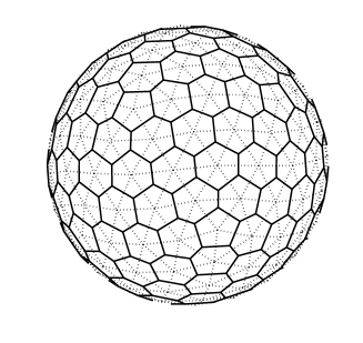
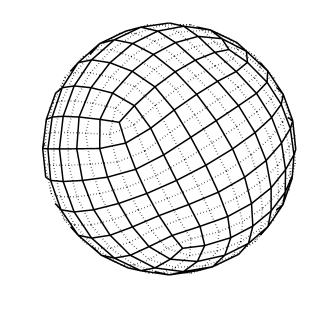
Figure 1: Left: a hexagonal–icosahedral mesh with 162 cells and 642 degrees of freedom. Right: a cubed-sphere mesh with 216 cells and 648 degrees of freedom. Continuous lines are primal mesh edges, dotted lines are dual mesh edges.

Any polygonal mesh has a corresponding dual mesh. (We will refer to the original mesh as the ‘primal’ mesh where necessary to distinguish it from the dual.) Each primal cell contains one dual vertex; each dual cell contains one primal vertex; each primal edge corresponds to one dual edge and these usually cross each other. Figure 1 shows both primal and dual edges for the two meshes.

3 Function spaces and compound finite elements

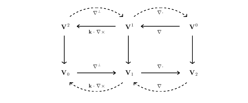
Figure 2: Schematic showing the function spaces used in the scheme and the relationships between them. Primal function spaces are on the bottom row and dual function spaces are on the top row.

The mimetic properties of the scheme arise from the relationships between the finite element function spaces. Three function spaces are used on the primal mesh ($\mathbf{V}_{0}$, $\mathbf{V}_{1}$, and $\mathbf{V}_{2}$), and three on the dual mesh ($\mathbf{V}^{2}$, $\mathbf{V}^{1}$, and $\mathbf{V}^{0}$). Figure 2 indicates that $\nabla^{\perp}$ (i.e. $\mathbf{k}\times\nabla$) maps from $\mathbf{V}_{0}$ to $\mathbf{V}_{1}$ and $\nabla\cdot$ maps from $\mathbf{V}_{1}$ to $\mathbf{V}_{2}$. More precisely, the primal function spaces satisfy the following properties.

Property List 1

• $\mathbf{u}\in\mathbf{V}_{1}\ \ \Rightarrow\ \ \nabla\cdot\mathbf{u}\in\mathbf{V}_{2}$.

• $\phi\in\mathbf{V}_{2}$ with $\int\phi\,dA=0\ \ \Rightarrow\ \ \exists\,\mathbf{u}\in\mathbf{V}_{1}\mathrm{\ st\ }\nabla\cdot\mathbf{u}=\phi$.

• $\psi\in\mathbf{V}_{0}\ \ \Rightarrow\ \ \nabla^{\perp}\psi\in\mathbf{V}_{1}$.

• $\forall\psi\in\mathbf{V}_{0},\ \nabla\cdot\nabla^{\perp}\psi=0$, and $\forall\mathbf{u}\in\mathbf{V}_{1}\ \mathrm{st}\ \nabla\cdot\mathbf{u}=0,\ \exists\,\psi\in\mathbf{V}_{0}\ \mathrm{st}\ \mathbf{u}=\nabla^{\perp}\psi$. That is, $\nabla^{\perp}$ maps onto the kernel of $\nabla\cdot$ .

The second condition assumes spherical geometry so that there are no lateral boundaries. The same assumption will be made throughout this paper; in particular, no boundary terms will arise when integrating by parts.

In a similar way, Fig. 2 indicates that $\nabla$ maps from $\mathbf{V}^{0}$ to $\mathbf{V}^{1}$ and $\mathbf{k}\cdot\nabla\times$ maps from $\mathbf{V}^{1}$ to $\mathbf{V}^{2}$. More precisely, the dual function spaces satisfy the following properties.

Property List 2

• $\hat{\mathbf{u}}\in\mathbf{V}^{1}\ \ \Rightarrow\ \ \mathbf{k}\cdot\nabla\times\hat{\mathbf{u}}\in\mathbf{V}^{2}$.

• $\hat{\xi}\in\mathbf{V}^{2}$ with $\int\hat{\xi}\,dA=0\ \ \Rightarrow\ \ \exists\,\hat{\mathbf{u}}\in\mathbf{V}^{1}\mathrm{\ st\ }\mathbf{k}\cdot\nabla\times\hat{\mathbf{u}}=\hat{\xi}$.

• $\hat{\chi}\in\mathbf{V}^{0}\ \ \Rightarrow\ \ \nabla\hat{\chi}\in\mathbf{V}^{1}$.

• $\forall\hat{\chi}\in\mathbf{V}^{0},\ \mathbf{k}\cdot\nabla\times\nabla\hat{\chi}=0$, and $\forall\hat{\mathbf{u}}\in\mathbf{V}^{1}\ \mathrm{st}\ \mathbf{k}\cdot\nabla\times\hat{\mathbf{u}}=0,\ \exists\,\hat{\chi}\in\mathbf{V}^{0}\ \mathrm{st}\ \hat{\mathbf{u}}=\nabla\hat{\chi}$. That is, $\nabla$ maps onto the kernel of $\mathbf{k}\cdot\nabla\times$ .

As noted earlier, standard finite element schemes in two dimensions typically use triangular or quadrilateral elements. Several families of mixed finite elements that satisfy Property List 1 on such meshes are known. However, in order to apply our scheme on more general polygonal meshes we will need to define families of mixed finite elements satisfying Property List 1 on those meshes. One way to do this is to use compound elements. Any polygonal element can be subdivided into a number of triangular subelements. A basis function on the polygonal element can then be defined as a suitable linear combination of basis functions on the subelements. The allowed linear combinations are determined by the requirement to satisfy Property List 1 or 2; see below.

The desire to use a dual mesh increases the need for finite element spaces on polygons, and hence for compound elements. Only in special cases (such as the cubed sphere, Fig. 1) can both the primal and dual meshes be built of triangles and quadrilaterals; other cases require higher degree polygons for either the primal or dual mesh (or both).

For a triangular primal mesh, Buffa and Christiansen (2007) describe a scheme for the construction of a dual hierarchy of function spaces. The dual mesh elements are compound elements, similar, though not identical, to those used here. However, their scheme is limited to the case of a triangular primal mesh and a barycentric refinement for the construction of the dual.

In a complementary study, Christiansen (2008) describes how finite element basis functions satifying Property List 1 may be constructed on arbitrary polygonal elements, without the need to divide into subelements, through a process of harmonic extension. For example, let $\gamma_{j}$ be a basis function for $\mathbf{V}_{0}$ associated with primal vertex $j$. Define $\gamma_{j}$ to equal $1$ at vertex $j$ and zero at all other vertices. Next extend $\gamma_{j}$ harmonically along primal mesh edges; that is, its second derivative should vanish so that its gradient is constant along each edge. Then extend $\gamma_{j}$ harmonically into the interior of each element; that is, solve

$$\nabla^{2}\gamma_{j}=0$$ (3)

subject to the Dirichlet boundary conditions given by the known values of $\gamma_{j}$ on element edges. In a similar way, let $\mathbf{v}_{e}$ be a basis function for $\mathbf{V}_{1}$ associated with edge $e$. Define the normal component of $\mathbf{v}_{e}$ to be a nonzero constant along edge $e$ (some arbitrary sign convention must be chosen to define the positive direction) and zero at all other edges. Then extend $\mathbf{v}_{e}$ harmonically into the interior of each element; that is, solve

$$\nabla\left(\nabla\cdot\mathbf{v}_{e}\right)=0$$ (4)

and

$$\nabla^{\perp}\left(\mathbf{k}\cdot\nabla\times\mathbf{v}_{e}\right)=0$$ (5)

subject to the known values of the normal component at element edges, for example by writing $\mathbf{v}_{e}=\nabla\phi+\nabla^{\perp}\psi$, implying $\nabla^{2}\phi=c_{1}$ and $\nabla^{2}\psi=c_{2}$ for constants $c_{1}$ and $c_{2}$. The boundary conditions determine the value of $c_{1}$, but not $c_{2}$. However, condition (3) along with the fourth property in List 1 implies that we must choose $c_{2}=0$, so that (5) reduces to

$$\mathbf{k}\cdot\nabla\times\mathbf{v}_{e}=0.$$ (6)

For the last function space $\mathbf{V}_{2}$ the basis function associated with cell $i$ is defined to be a nonzero constant in cell $i$ and zero in all other cells. It may then be verified that the properties in List 1 do indeed hold for the spaces spanned by these basis functions.

Although the harmonic extension approach provides a general method for constructing the lowest order mimetic finite element spaces on polygonal meshes, its drawback is that, except for the simplest element shapes, the basis functions cannot be found analytically. Even if they are found numerically, the inner products required for the finite element method cannot be computed exactly, either analytically or by numerical quadrature.

Here we take inspiration from both Buffa and Christiansen (2007) and Christiansen (2008) to construct spaces of compound finite elements for arbitrary polygonal primal and dual meshes, by a process that might be called discrete harmonic extension. For the function spaces on the primal mesh, in effect, we solve a finite element discretization of (3), (4), and (6) on the mesh of triangular subelements in order to construct the compound basis elements for the original polygonal mesh. For this discretization we use the lowest order mimetic finite element spaces on the triangular subelements, in which $\mathbf{V}_{0}$ comprises continuous piecewise linear elements, $\mathbf{V}_{1}$ comprises the lowest order Raviart-Thomas elements, and $\mathbf{V}_{2}$ comprises piecewise constant elements; $\text{P1-RT0-P0}^{\text{DG}}$ in standard shorthand. Although only discrete versions of (3), (4), and (6) are solved, it may be verified that the properties in List 1 hold exactly. The basis functions on the triangular subelements are known analytically, and the compound elements are linear combinations of these; therefore, integrals of products of basis functions, for example to compute entries of a mass matrix, can all be computed exactly.

The resulting compound elements provide a generalization to polygonal meshes of the $\text{P1-RT0-P0}^{\text{DG}}$ hierarchy of spaces, so we will refer to them as compound $\text{P1-RT0-P0}^{\text{DG}}$ elements. Like the non-compound spaces described by Christiansen (2008), the expansion coefficients for $\mathbf{V}_{0}$ correspond to mesh vertices, for $\mathbf{V}_{1}$ to edges, and for $\mathbf{V}_{2}$ to cells. Thus, this hierarchy provides a finite element analogue of the polygonal C-grid if we choose to represent velocity in $\mathbf{V}_{1}$ and the mass variable in $\mathbf{V}_{2}$.

The construction of basis elements for the dual spaces proceeds in a very similar way, except that the basis function for $\mathbf{V^{1}}$ is given by $\mathbf{k}\times$ the solution of (4) and (6). This gives rise to a compound $\text{P1-N0-P0}^{\text{DG}}$ hierarchy of spaces, where N0 refers to the lowest order two-dimensional Nédélec elements.

An important detail concerns the number of subelements needed. It may appear natural to subdivide an $n$-gon cell into $n$ triangular subelements. However, it will be necessary to calculate integrals on the overlap between primal and dual elements (section 4.2). In order to be able to do this when the domain is a curved surface approximated by plane triangular subelement facets, both the primal and dual compound element meshes must be built from triangular subelements of the the same supermesh. To achieve this we divide $n$-gon cells (whether primal or dual) into $2n$ subelements (Fig. 3).

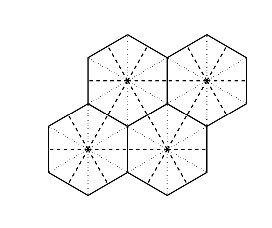
Figure 3: Example of part of a hexagonal primal mesh (solid lines) with its triangular dual mesh (dashed lines) and the supermesh of triangular subelements (all lines) used to construct the compound elements.

It is convenient to normalize the basis functions as follows:

$$\alpha_{i}\in\mathbf{V}_{2}: \int_{\mathrm{cell}\ i^{\prime}}\alpha_{i}\,dA=\delta_{i\,i^{\prime}};$$ (7)

$$\mathbf{v}_{e}\in\mathbf{V}_{1}: \int_{\mathrm{edge}\ e^{\prime}}\mathbf{v}_{e}\cdot\mathbf{n}\,dl=\delta_{e\,e^{\prime}};$$ (8)

$$\gamma_{j}\in\mathbf{V}_{0}: \left.\gamma_{j}\right|_{\mathrm{vertex}\ j^{\prime}}=\delta_{j\,j^{\prime}};$$ (9)

$$\beta_{j}\in\mathbf{V}^{2}: \int_{\mathrm{dualcell}\ j^{\prime}}\beta_{j}\,dA=\delta_{j\,j^{\prime}};$$ (10)

$$\mathbf{w}_{e}\in\mathbf{V}^{1}: \int_{\mathrm{dualedge}\ e^{\prime}}\mathbf{w}_{e}\cdot\mathbf{m}\,dl=\delta_{e\,e^{\prime}};$$ (11)

$$\chi_{i}\in\mathbf{V}^{0}: \left.\chi_{i}\right|_{\mathrm{dual\ vertex}\ i^{\prime}}=\delta_{i\,i^{\prime}}.$$ (12)

Here $\mathbf{n}$ is the unit normal vector to primal edge $e$ and $\mathbf{m}$ is the unit tangent vector to dual edge $e$, with $\mathbf{m}$ and $\mathbf{n}$ pointing in the same sense (i.e. $\mathbf{n}\cdot\mathbf{m}>0$, though they need not be parallel if the dual edges are not orthogonal to the primal edges), as in Thuburn and Cotter (2012). The normalization is chosen so that degrees of freedom for fields in $\mathbf{V}_{2}$ and $\mathbf{V}^{2}$ correspond to area integrals of scalars over primal cells and dual cells, respectively, degrees of freedom for a field in $\mathbf{V}_{1}$ correspond to normal fluxes integrated along primal edges, degrees of freedom in $\mathbf{V}^{1}$ correspond to circulations integrated along dual edges, and degrees of freedom for fields in $\mathbf{V}_{0}$ and $\mathbf{V}^{0}$ correspond to nodal values of scalars at primal vertices and dual vertices respectively. Again, this corresponds closely to the framework of Thuburn and Cotter (2012).

Melvin and Thuburn (2014) have analyzed the wave dispersion properties for finite element discretizations of the linear shallow water equations using these compound elements. That paper gives explicit expressions for the $\mathbf{V}_{1}$ and $\mathbf{V}_{2}$ compound element basis functions for the cases of a square mesh and a regular hexagonal mesh on a plane. For more general meshes it is straightforward and convenient to construct the compound element basis functions numerically. Figure 4 shows typical basis elements for the three primal mesh function spaces for quadrilateral and hexagonal cells.

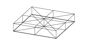
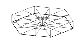
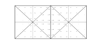
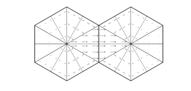
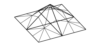
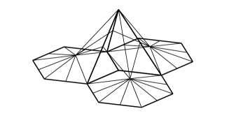
Figure 4: Typical compound basis elements of the function spaces on a square mesh (left) and a hexagonal mesh (right). structures. Top row $\alpha_{i}\in\mathbf{V}_{2}$; middle row $\mathbf{v}_{e}\in\mathbf{V}_{1}$; bottom row $\gamma_{j}\in\mathbf{V}_{0}$. In the middle row, at subelement edges the normal components of the basis vectors are continuous.

The fields used in the computation are represented as expansions in terms of these basis elements. For example,

$$\phi=\sum_{i}\phi_{i}\alpha_{i} \ \ \ \ \ \in\mathbf{V}_{2},$$ (13)

$$\mathbf{u}=\sum_{e}u_{e}\mathbf{v}_{e} \ \ \ \ \ \in\mathbf{V}_{1}$$ (14)

for the prognostic geopotential and velocity fields, and

$$\xi=\sum_{j}\xi_{j}\gamma_{j}\ \ \ \ \ \in\mathbf{V}_{0}$$ (15)

for the relative vorticity field. Here the sums are global sums over all basis elements in the relevant spaces. In some cases it will be useful to introduce dual space representations of fields; these will be indicated by a hat symbol where necessary to distinguish them from the corresponding primal space representations. For example,

$$\hat{\phi}=\sum_{i}\hat{\phi}_{i}\chi_{i} \ \ \ \ \ \in\mathbf{V}^{0},$$ (16)

$$\hat{\mathbf{u}}=\sum_{e}\hat{u}_{e}\mathbf{w}_{e} \ \ \ \ \ \in\mathbf{V}^{1},$$ (17)

$$\hat{\xi}=\sum_{j}\hat{\xi}_{j}\beta_{j} \ \ \ \ \ \in\mathbf{V}^{2}.$$ (18)

The fields $\phi$ and $\hat{\phi}$ have the same number of degrees of freedom, and it is possible construct a well-conditioned and reversible map between them by demanding that they agree when integrated against any test function in the primal space $\mathbf{V}_{2}$. Similarly, the fields $\mathbf{u}$ and $\hat{\mathbf{u}}$ have the same number of degrees of freedom, and it is possible construct a well-conditioned and reversible map between them by demanding that they agree when integrated against any test function in the primal space $\mathbf{V}_{1}$. It will also be useful to introduce spatially averaged versions of some fields. For example,

$$\widetilde{\phi}=\sum_{j}\widetilde{\phi}_{j}\gamma_{j} \ \ \ \ \ \in\mathbf{V}_{0},$$ (19)

$$\overline{\phi}=\sum_{j}\overline{\phi}_{j}\beta_{j} \ \ \ \ \ \in\mathbf{V}^{2}.$$ (20)

Here, $\widetilde{\phi}$ and $\overline{\phi}$ have the same number of degrees of freedom, and it is possible construct a well-conditioned and reversible map between them by demanding that they agree when integrated against any test function in the primal space $\mathbf{V}_{0}$. $\widetilde{\phi}$ or $\overline{\phi}$ can be obtained from $\phi$ by demanding that they agree when integrated against any test function in $\mathbf{V}_{0}$; in effect this provides an averaging operation from $\mathbf{V}_{2}$ to $\mathbf{V}_{0}$ or $\mathbf{V}^{2}$. (However, we should not expect to be able to obtain $\phi$ from $\widetilde{\phi}$ or $\overline{\phi}$, as this would require an un-averaging operation, which will be ill-conditioned if it exists at all.)

It will be convenient to be able to refer to the vector of degrees of freedom for any field. To do this, we will use the same letter (with hat, tilde or bar if needed) but in upper case. Thus, for example, $\Phi$ will be the vector of values $(\phi_{1},\phi_{2},\dots)^{T}$, $\hat{U}$ will be the vector of values $(\hat{u}_{1},\hat{u}_{2},\ldots)^{T}$, etc.

4 Finite element scheme

Finite element schemes solve the governing equations by approximating the solution in the chosen function spaces, written as expansions in terms of basis functions (e.g. (13), (14)), and demanding that the equations be satisfied in weak form, that is, when multiplied by any test function in the appropriate space and integrated over the domain. In this approach (1) becomes

$$\int\alpha_{i}\left(\phi_{t}+\nabla\cdot\mathbf{f}\right)\,dA=0\ \ \ \ \forall\alpha_{i}\in\mathbf{V}_{2},$$ (21)

or, regarding the integral as an inner product for which we introduce angle backet notation,

$$\langle\alpha_{i},\phi_{t}\rangle+\langle\alpha_{i},\nabla\cdot\mathbf{f}\rangle=0\ \ \ \ \forall\alpha_{i}\in\mathbf{V}_{2}.$$ (22)

Similarly, (2) becomes

$$\int\mathbf{v}_{e}\cdot\left\{\mathbf{u}_{t}+\mathbf{q}^{\perp}+\nabla(\phi_{\mathrm{T}}+k)\right\}\,dA=0\ \ \ \ \forall\mathbf{v}_{e}\in\mathbf{V}_{1},$$ (23)

or

$$\langle\mathbf{v}_{e},\mathbf{u}_{t}\rangle+\langle\mathbf{v}_{e},\mathbf{q}^{\perp}\rangle+\langle\mathbf{v}_{e},\nabla(\phi_{\mathrm{T}}+k)\rangle=0.$$ (24)

(The construction of the nonlinear terms $\mathbf{f}$, $\mathbf{q}$ and $k$ is discussed in section 4.6 below.) The method generally leads to a system of algebraic equations for the unknown coefficients in the expansion of the solution.

The following subsections show how the mimetic finite element method can be re-expressed in terms of certain matrix operators acting on the coefficient vectors $\Phi$, $U$, etc. The notation is chosen to highlight the similarity to the finite volume scheme of Thuburn et al. (2014).

4.1 Matrix representation of derivatives – strong derivatives

The velocity basis elements are constructed and normalized so as to have constant divergence over the cell upwind of the edge where the degree of freedom resides, with area integral equal to $1$, and constant divergence over the cell downwind of this edge, with area integral equal to $-1$, with zero velocity and hence zero divergence in all other cells. Thus

$$\nabla\cdot\mathbf{v}_{e}=\sum_{i}n_{e\,i}\alpha_{i}\ \ \ \ \ \in\mathbf{V}_{2},$$ (25)

where $n_{e\,i}$ is equal to $1$ when the normal at edge $e$ points out of cell $i$, equal to $-1$ when the normal at edge $e$ points into cell $i$, and is zero otherwise. We will write $D_{2}$ for the matrix whose transpose has components $n_{e\,i}$. $D_{2}$ is called an incidence matrix because it describes some aspects of the grid topology. Hence, the divergence $\delta$ of an arbitrary velocity field $\mathbf{u}$ is

$$\sum_{i}\delta_{i}\alpha_{i}=\delta=\nabla\cdot\mathbf{u}=\sum_{e}u_{e}\nabla\cdot\mathbf{v}_{e}=\sum_{e\,i}u_{e}n_{e\,i}\alpha_{i}.$$ (26)

Equating coefficients of $\alpha_{i}$ gives

$$\delta_{i}=\sum_{e}n_{e\,i}u_{e},$$ (27)

or, in matrix-vector notation

$$\Delta=D_{2}U.$$ (28)

Note we could have demanded that (26) should hold when integrated against any test function in $\mathbf{V}_{2}$, to obtain the same result. However, this would obscure the fact that (26) actually holds at every point in the domain (except on cell edges where all terms are discontinuous), not just when integrated against a test function. In this sense, $\nabla\cdot\,:\mathbf{V}_{1}\rightarrow\mathbf{V}_{2}$ is a strong derivative operator.

Similarly, the basis elements in $\mathbf{V}_{0}$ are constructed so that

$$\nabla^{\perp}\gamma_{j}=\sum_{e}-t_{e\,j}\mathbf{v}_{e},$$ (29)

where $t_{e\,j}$ is defined to equal $1$ if edge $e$ is incident on vertex $j$ and the unit tangent vector $\mathbf{t}$ at edge $e$ points towards vertex $j$, $-1$ if it points away from vertex $j$, and zero otherwise. The unit normal and unit tangent at any edge are related by $\mathbf{t}=\mathbf{k}\times\mathbf{n}$. Hence, a stream function $\psi$ is related to the corresponding rotational velocity field $\mathbf{u}$ by

$$\sum_{e}u_{e}\mathbf{v}_{e}=\mathbf{u}=\nabla^{\perp}\psi=\sum_{j}\psi_{j}\nabla^{\perp}\gamma_{j}=\sum_{j\,e}-\psi_{j}t_{e\,j}\mathbf{v}_{e}.$$ (30)

Equating coefficients of $\mathbf{v}_{e}$ and defining $D_{1}$ to be the matrix whose entries are $t_{e\,j}$ gives the matrix-vector form

$$U=-D_{1}\Psi.$$ (31)

Equation (30) holds pointwise (again with the exception of discontinuities), so $\nabla^{\perp}:\mathbf{V}_{0}\rightarrow\mathbf{V}_{1}$ is a strong derivative operator.

The matrices $D_{1}$ and $D_{2}$ are exactly the same as in the finite volume framework of Thuburn and Cotter (2012). In particular, they have the property that

$$D_{2}D_{1}\equiv 0,$$ (32)

giving a discrete analogue of the continuous property $\nabla\cdot\nabla^{\perp}\equiv 0$.

Analogous relations hold on the dual spaces.

$$\nabla\chi_{i}=-\sum_{e}n_{e\,i}\mathbf{w}_{e}$$ (33)

implies that the discrete analogue of

$$\hat{\mathbf{u}}=\nabla\hat{p}$$ (34)

is

$$\hat{U}=\overline{D}_{1}\hat{P},$$ (35)

where $\overline{D}_{1}=-D_{2}^{T}$. Similarly

$$\mathbf{k}\cdot\nabla\times\mathbf{w}_{e}=\sum_{j}t_{e\,j}\beta_{j}$$ (36)

implies that the discrete analogue of

$$\hat{\xi}=\mathbf{k}\cdot\nabla\times\hat{\mathbf{u}}$$ (37)

is

$$\hat{\Xi}=\overline{D}_{2}\hat{U},$$ (38)

where $\overline{D}_{2}=D_{1}^{T}$. Again, these are strong derivative operators.

The matrices $\overline{D}_{1}$ and $\overline{D}_{2}$ have the property

$$\overline{D}_{2}\overline{D}_{1}\equiv 0,$$ (39)

giving a discrete analogue in the dual space of the continuous relation $\mathbf{k}\cdot\nabla\times\nabla\equiv 0$.

4.2 Mass matrices and other operators

Define the following mass matrices for the primal function spaces:

$$L_{i\,i^{\prime}}=\langle\alpha_{i},\alpha_{i^{\prime}}\rangle=\int\alpha_{i}\alpha_{i^{\prime}}\,dA, (\mathbf{V}_{2}\rightarrow\mathbf{V}_{2}),$$ (40)

$$M_{e\,e^{\prime}}=\langle\mathbf{v}_{e},\mathbf{v}_{e^{\prime}}\rangle=\int\mathbf{v}_{e}\cdot\mathbf{v}_{e^{\prime}}\,dA, (\mathbf{V}_{1}\rightarrow\mathbf{V}_{1}),$$ (41)

$$N_{j\,j^{\prime}}=\langle\gamma_{j},\gamma_{j^{\prime}}\rangle=\int\gamma_{j}\gamma_{j^{\prime}}\,dA, (\mathbf{V}_{0}\rightarrow\mathbf{V}_{0}).$$ (42)

The expressions in parentheses indicate that $L$ maps $\mathbf{V}_{2}$ to itself, etc. (Analogous mass matrices may be defined for the dual spaces; however, they will not be needed here.)

The following matrices are also needed.

$$R_{j\,i}=\langle\gamma_{j},\alpha_{i}\rangle, (\mathbf{V}_{2}\rightarrow\mathbf{V}_{0}),$$ (43)

$$W_{e\,e^{\prime}}=-\langle\mathbf{v}_{e},\mathbf{v}_{e^{\prime}}^{\perp}\rangle=-W_{e^{\prime}\,e}, (\mathbf{V}_{1}\rightarrow\mathbf{V}_{1}),$$ (44)

$$H_{e\,e^{\prime}}=\langle\mathbf{v}_{e},\mathbf{w}_{e^{\prime}}\rangle, (\mathbf{V}^{1}\rightarrow\mathbf{V}_{1}),$$ (45)

$$J_{j\,j^{\prime}}=\langle\gamma_{j},\beta_{j^{\prime}}\rangle, (\mathbf{V}^{2}\rightarrow\mathbf{V}_{0}).$$ (46)

For completeness we may also define

$$I_{i\,i^{\prime}}=\langle\alpha_{i},\chi_{i^{\prime}}\rangle,\ \ \ \ \ (\mathbf{V}^{0}\rightarrow\mathbf{V}_{2}),$$ (47)

though we will not need to employ this matrix in the shallow water scheme.

One further operator will be needed to construct the kinetic energy per unit mass. It is

$$T_{i\,e\,e^{\prime}}=\int_{\mathrm{cell}\ i}\mathbf{v}_{e}\cdot\mathbf{v}_{e^{\prime}}\,dA=A_{i}\langle\alpha_{i},\mathbf{v}_{e}\cdot\mathbf{v}_{e^{\prime}}\rangle\ \ \ \ \ (\mathbf{V}_{1}\otimes\mathbf{V}_{1}\rightarrow\mathbf{V}_{2}).$$ (48)

where $A_{i}=(L_{i\,i})^{-1}$ is the area of primal cell $i$.

All of these matrices can be precomputed, so that no quadrature needs to be done at run time. Moreover, they are all sparse, so they can be efficiently stored as lists of stencils and coefficients.

Let $U^{\perp}$ be the coefficients of the expansion of the projection of $\mathbf{u}^{\perp}$ into $\mathbf{V}_{1}$:

$$\langle\mathbf{v}_{e},\sum_{e^{\prime}}U^{\perp}_{e^{\prime}}\mathbf{v}_{e^{\prime}}\rangle=\langle\mathbf{v}_{e},\sum_{e^{\prime}}U_{e^{\prime}}\mathbf{v}^{\perp}_{e^{\prime}}\rangle=\langle\mathbf{v}_{e},\mathbf{u}^{\perp}\rangle~{}~{}~{}~{}~{}~{}~{}~{}\forall\mathbf{v}_{e}\in\mathbf{V}_{1}.$$ (49)

Using (41) and (44) gives the discrete version of the $\perp$ operator:

$$MU^{\perp}=-WU.$$ (50)

Demanding agreement between (13) and (16) when integrated against any test function in $\mathbf{V}_{2}$ leads to

$$L\Phi=I\hat{\Phi}.$$ (51)

Similarly, demanding agreement between (14) and (17) when integrated against any test function in $\mathbf{V}_{1}$ gives

$$MU=H\hat{U},$$ (52)

while demanding agreement between (15) and (18) when integrated against any test function in $\mathbf{V}_{0}$ gives

$$N\Xi=J\hat{\Xi}.$$ (53)

The relations (51), (52), (53) provide invertible maps between the primal and dual function spaces. Thus, they are examples of discrete Hodge star operators (e.g. Hiptmair, 2001). They may be contrasted with the analogous relations employed by Thuburn and Cotter (2012) and Thuburn et al. (2014) for the finite volume case, which do not involve mass matrices.

Demanding agreement between (13), (19), and (20) when integrated against any test function in $\mathbf{V}_{0}$ leads to

$$N\widetilde{\Phi}=J\overline{\Phi}=R\Phi.$$ (54)

This is the matrix representation of the averaging operator discussed in section 3.

4.3 Matrix representation of derivatives – weak derivatives

A field in $\mathbf{V}_{2}$ is discontinuous, so its gradient in $\mathbf{V}_{1}$ can only be defined in a weak sense, by integrating against all test functions in $\mathbf{V}_{1}$. For example,

$$\mathbf{g}=\nabla\phi$$ (55)

must be approximated as

$$\langle\mathbf{v}_{e},\mathbf{g}\rangle=\langle\mathbf{v}_{e},\nabla\phi\rangle\ \ \forall\mathbf{v}_{e}\in\mathbf{V}_{1},$$ (56)

where $\phi\in\mathbf{V}_{2}$, $\mathbf{g}\in\mathbf{V}_{1}$. Expanding both $\phi$ and $\mathbf{g}$ in terms of basis elements and integrating by parts then leads to the matrix form

$$MG=\overline{D}_{1}L\Phi.$$ (57)

Similarly, the curl of a vector field in $\mathbf{V}_{1}$ must be defined by integration against all test functions in $\mathbf{V}_{0}$. For example, the discrete analogue of

$$\xi=\mathbf{k}\cdot\nabla\times\mathbf{u},$$ (58)

after expanding in basis functions and integrating by parts, is

$$N\Xi=\overline{D}_{2}MU.$$ (59)

Combining these two results, the discrete analogue of

$$z=\mathbf{k}\cdot\nabla\times\nabla\phi$$ (60)

is

$$NZ=\overline{D}_{2}\overline{D}_{1}L\Phi,$$ (61)

which is identically zero.

These derivative operators can be combined to obtain the Laplacian of a scalar. For a scalar $\phi\in\mathbf{V}_{2}$, the discrete Laplacian is $D_{2}M^{-1}\overline{D}_{1}L\Phi$. For a scalar $\psi\in\mathbf{V}_{0}$, the discrete Laplacian is $-N^{-1}\overline{D}_{2}MD_{1}\Psi$. The operators introduced above lead to a discrete version of the Helmholtz decomposition, in which an arbitrary vector field is decomposed into its divergent and rotational parts:

$$U=M^{-1}\overline{D}_{1}L\Phi-D_{1}\Psi.$$ (62)

Figure 5 summarizes how the operators introduced here map between the different function spaces.

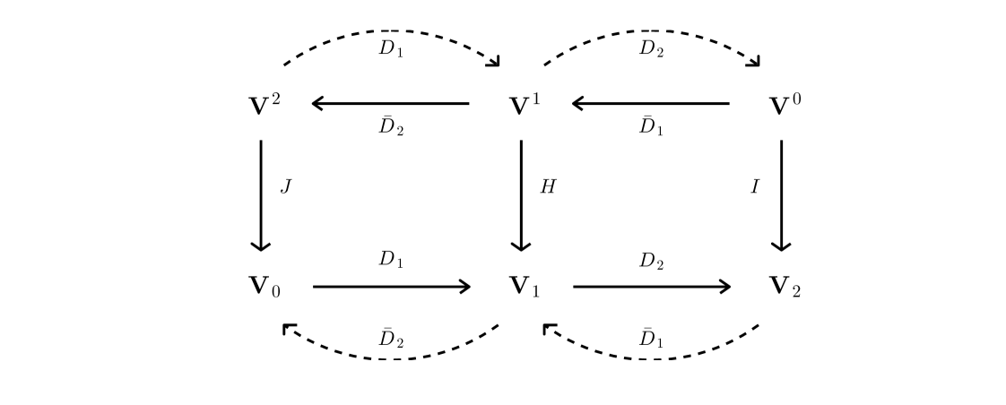
Figure 5: Schematic showing the function spaces used in the scheme and how the various matrices introduced above map between them.

4.4 Some operator identities

The operators defined above satisfy some key relations that underpin the mimetic properties of the scheme. We have already seen that

$${D}_{2}{D}_{1}\equiv 0$$ (63)

and

$$\overline{D}_{2}\overline{D}_{1}\equiv 0,$$ (64)

leading to discrete analogues of $\nabla\cdot\nabla^{\perp}\equiv 0$ and $\mathbf{k}\cdot\nabla\times\nabla\equiv 0$.

Next, note that the basis elements $\gamma_{j}$ give a partition of unity, that is

$$\sum_{j}\gamma_{j}=1$$ (65)

at every point in the domain. Consequently

$$\sum_{j}R_{j\,i}=\langle 1,\alpha_{i}\rangle=1$$ (66)

and

$$\sum_{j}J_{j\,j^{\prime}}=\langle 1,\beta_{j^{\prime}}\rangle=1.$$ (67)

Now let

$$\psi=\sum_{j}\psi_{j}\gamma_{j}\ \ \in\mathbf{V}_{0}.$$ (68)

By considering the projection of $\nabla\psi$ into $\mathbf{V}_{1}$

$$\langle\mathbf{v}_{e},(\nabla^{\perp}\psi)^{\perp}\rangle=-\langle\mathbf{v}_{e},\nabla\psi\rangle$$ (69)

and integrating by parts and using the matrices defined in sections 4.1 and 4.2, we obtain

$$-\overline{D}_{2}W=RD_{2}.$$ (70)

This identity is key to obtaining the steady geostrophic mode property (section 4.5.3 below). A rough interpretation is that averaging velocities to construct the Coriolis terms ($W$) then taking their divergence ($\overline{D}_{2}$) gives the same result as computing the velocity divergence ($D_{2}$) followed by averaging to $\mathbf{V}_{0}$ ($R$). One consequence is $\overline{D}_{2}WD_{1}=-RD_{2}D_{1}\equiv 0$.

An identical formula to (70) relating $R$ and $W$ was obtained by Thuburn and Cotter (2012) for the finite volume case. The result was originally derived for the construction of the Coriolis terms on orthogonal grids by Thuburn et al. (2009), and Thuburn and Cotter (2012) showed that it could be embedded in a more general framework applicable to nonorthogonal grids. Moreover, Thuburn et al. (2009) showed that, for any given $R$ with the appropriate stencil (which we have here) and satisfying (66), there is a unique antisymmetric $W$ satisfying (70), and gave an explicit construction for $W$ in terms of $R$. Thus, although the context and interpretation are slightly different here, we can, nevertheless, use the Thuburn et al. construction in implementing the mixed finite-element version of the $W$ operator!

Now consider the two representations of any vector field $\mathbf{u}\in\mathbf{V}_{1}$, $\hat{\mathbf{u}}\in\mathbf{V}^{1}$ related by

$$\langle\mathbf{v},\mathbf{u}\rangle=\langle\mathbf{v},\hat{\mathbf{u}}\rangle\ \ \forall\mathbf{v}\in\mathbf{V}_{1},$$ (71)

so that

$$MU=H\hat{U}.$$ (72)

Since $\nabla^{\perp}\gamma_{j}\in\mathbf{V}_{1}$,

$$\langle\nabla^{\perp}\gamma_{j},\mathbf{u}\rangle=\langle\nabla^{\perp}\gamma_{j},\hat{\mathbf{u}}\rangle\ \ \forall\gamma_{j}\in\mathbf{V}_{0},$$ (73)

and integrating by parts gives

$$-\langle\gamma_{j},\mathbf{k}\cdot\nabla\times\mathbf{u}\rangle=-\langle\gamma_{j},\mathbf{k}\cdot\nabla\times\hat{\mathbf{u}}\rangle\ \ \forall\gamma_{j}\in\mathbf{V}_{0}.$$ (74)

Hence

$$-\overline{D}_{2}MU=-J\overline{D}_{2}\hat{U}.$$ (75)

Finally, substituting from (72) and noting that $\hat{U}$ is arbitrary gives

$$\overline{D}_{2}H=J\overline{D}_{2}.$$ (76)

The interpretation of this identity is that, for a velocity field in $\mathbf{V}^{1}$, taking the curl followed by mapping to the primal space is equivalent to mapping the velocity field to the primal space then taking its curl. One consequence is that $\overline{D}_{2}H\overline{D}_{1}=J\overline{D}_{2}\overline{D}_{1}\equiv 0$.

Finally, let $\chi\in\mathbf{V}_{2}$ and $\hat{\chi}\in\mathbf{V}^{0}$ be two discrete representations of a scalar field related by

$$\langle\alpha,\chi\rangle=\langle\alpha,\hat{\chi}\rangle\ \ \forall\alpha\in\mathbf{V}_{2},$$ (77)

so that

$$LX=I\hat{X}.$$ (78)

Since $\nabla\cdot\mathbf{v}_{e}\in\mathbf{V}_{2}$ for any $\mathbf{v}_{e}\in\mathbf{V}_{1}$, we have

$$\langle\nabla\cdot\mathbf{v}_{e},\chi\rangle = \langle\nabla\cdot\mathbf{v}_{e},\hat{\chi}\rangle,$$

$$\langle\mathbf{v}_{e},\nabla\chi\rangle = \langle\mathbf{v}_{e},\nabla\hat{\chi}\rangle,$$

$$\overline{D}_{1}LX = H\bar{D}_{1}\hat{X},$$ (79)

or, using (78) and noting that $\hat{X}$ is arbitrary,

$$\overline{D}_{1}I=H\overline{D}_{1}.$$ (80)

Using these identities and the Hodge star operators, it can be seen that taking a weak derivative in the primal space is equivalent to applying a Hodge star to map to the dual space, taking a strong derivative in the dual space, and applying another Hodge star to map back to the primal space:

$$M^{-1}\overline{D}_{1}L = (M^{-1}H)\,\overline{D}_{1}\,(I^{-1}L);$$ (81)

$$N^{-1}\overline{D}_{2}M = (N^{-1}J)\,\overline{D}_{2}\,(H^{-1}M)$$ (82)

(Cotter and Thuburn, 2014). Thus, certain paths in Fig. 5 commute. Weak derivative operators in the dual space can be defined by demanding a similar equivalence with primal space strong derivatives; however, the resulting formulas are less elegant and, in any case, will not be needed.

4.5 Linear shallow water equations

We first examine the spatial discretization of the linear shallow water equations to illustrate how some key conservation and balance properties arise. The rotating shallow water equations (1), (2) when linearized about a resting basic state with constant geopotential $\phi_{0}$ and with constant Coriolis parameter $f$ become

$$\phi_{t}+\nabla\cdot(\phi_{0}\mathbf{u}) = 0,$$ (83)

$$\mathbf{u}_{t}+f\mathbf{u}^{\perp}+\nabla\phi = 0.$$ (84)

By writing these in weak form (analogous to (22) and (24)), expanding $\phi$ and $\mathbf{u}$ in terms of basis functions, and using the notation and operators defined above, we obtain

$$\dot{\Phi}+\phi_{0}D_{2}U = 0,$$ (85)

$$M\dot{U}-fWU+\overline{D}_{1}L\Phi = 0.$$ (86)

4.5.1 Mass conservation

Mass conservation is trivially satisfied (for both the linear and nonlinear equations) because the discrete divergence is a strong operator, so the domain integral of the discrete divergence of any vector field vanishes.

4.5.2 Energy conservation

For the linearized equations the total energy is given by

$$E = \frac{1}{2}\int\phi^{2}+\phi_{0}\mathbf{u}\cdot\mathbf{u}\,dA$$ (87)

$$= \frac{1}{2}\Phi^{T}L\Phi+\frac{1}{2}\phi_{0}U^{T}MU.$$

Hence, the rate of change of total energy is

$$\frac{dE}{dt} = \Phi^{T}L\dot{\Phi}+\phi_{0}U^{T}M\dot{U}$$ (88)

$$= -\phi_{0}\Phi^{T}LD_{2}U+\phi_{0}U^{T}(fWU-\overline{D}_{1}L\Phi)$$

$$= 0,$$

where we have used the fact that $L$ and $M$ are symmetric, $W$ is antisymmetric, and $D_{2}^{T}=-\overline{D}_{1}$.

4.5.3 Steady geostrophic modes

The linear shallow water equations support steady non-divergent flows in geostrophic balance. A numerical method must respect this property in order to be able to represent geostrophic balance. However, it is non-trivial to achieve this property because several ingredients must fall into place.

• The geopotential $\phi$ must be steady. The steadiness of $\phi$ follows immediately from the assumption that $\nabla\cdot\mathbf{u}=0$.

• The relative vorticity $\xi$ must be steady; neither the pressure gradient nor the Coriolis term should generate vorticity. First note that, from Property List 1, $U=-D_{1}\Psi$ for some $\Psi$. Taking the curl of the momentum equation then gives

  $$N\dot{\Xi}=\overline{D}_{2}M\dot{U}=\overline{D}_{2}(-fWD_{1}\Psi-\overline{D}_{1}L\Phi).$$ (89)

  The pressure gradient term does not contribute because $\overline{D}_{2}\overline{D}_{1}\equiv 0$, and the Coriolis term does not contribute because $\overline{D}_{2}WD_{1}\equiv 0$.

• There must exist a geopotential $\phi$ that balances the Coriolis term so that the divergence is steady. Taking the divergence of the momentum equation gives the divergence tendency

  $$\dot{\Delta}=D_{2}M^{-1}(-fWD_{1}\Psi-\overline{D}_{1}\Phi).$$ (90)

  If we define $\Phi=fL^{-1}R^{T}\Psi$ and use the transpose of (70) we find that $\dot{\Delta}$ does indeed vanish; thus the required $\phi$ does exist.

Consequently, the scheme does support steady geostrophic modes for the linearized equations. (Note, it is not necessarily true that any given $\phi$ field can be balanced by some non-divergent velocity field. On some meshes, particularly those with triangular primal cells, there might not be enough velocity degrees of freedom to balance all possible $\phi$ fields.)

4.5.4 Linear PV equation

A generalization of the steady geostrophic mode property is that the scheme should have a suitable PV equation. In this section we consider the linear case; the nonlinear case is dealt with in section 4.6.3.

The mass field $\phi$ and the vorticity field $\xi$ live in different spaces. To construct a suitable discrete PV we need an averaged mass field $\widetilde{\phi}$ that lives in the same space as $\xi$. The linearized PV should be independent of time. For this to hold, $\xi$ and $\widetilde{\phi}$ must see the same divergence field.

For a general (possibly divergent) velocity field $\mathbf{u}$, the vorticity equation (89) becomes

$$N\dot{\Xi}=f\overline{D}_{2}WU.$$ (91)

Define $\widetilde{\phi}$ using (54). Then the evolution of $\widetilde{\phi}$ is given by

$$N\dot{\widetilde{\Phi}} = R\dot{\Phi}$$ (92)

$$= -\phi_{0}RD_{2}U$$

$$= \phi_{0}\overline{D}_{2}WU,$$

(using (70)). Thus, $\Xi$ and $\widetilde{\Phi}$ see the same divergence $-\overline{D}_{2}WU$; consequently the linearized PV $\Xi/\phi_{0}-f\widetilde{\Phi}/\phi_{0}^{2}$ is independent of time.

4.6 Nonlinear shallow water equations

The nonlinear rotating shallow water equations are (1) and (2). Writing these in weak form (22) and (24), and letting $F$, $Q$, and $K$ be the vectors of coefficients for the discrete representations of the mass flux $\mathbf{f}=\mathbf{u}\phi$, the PV flux $\mathbf{q}=\mathbf{f}\pi$, and the kinetic energy per unit mass $k=\mathbf{u}\cdot\mathbf{u}/2$, the nonlinear discretization becomes

$$\dot{\Phi}+D_{2}F = 0,$$ (93)

$$M\dot{U}+MQ^{\perp}+\overline{D}_{1}L(\Phi_{T}+K) = 0.$$ (94)

The remaining issue is how to construct suitable values of the three nonlinear terms $K$, $F$, and $Q^{\perp}$.

4.6.1 Constructing $K$

The discretization of $k$ follows the standard finite element construction, which is to project $\nabla k$ into $\mathbf{V}_{1}$. It may easily be verified that this is equivalent to projecting $k$ into $\mathbf{V}_{2}$ before taking the weak gradient. Using the $T$ operator defined in section 4.2, the expansion coefficients $K$ of the projected $k$ are given by

$$k_{i}=\frac{1}{2}\sum_{e\,e^{\prime}}T_{i\,e\,e^{\prime}}u_{e}u_{e^{\prime}}.$$ (95)

4.6.2 Constructing $F$

Because the $\phi$ field is approximated as piecewise constant, its degrees of freedom can be interpreted as primal cell integrals. Similarly, the degrees of freedom of the $\mathbf{u}$ field are the integrals of the normal velocity fluxes across primal cell edges, and the $D_{2}$ operator looks exactly like a finite volume divergence operator. Thus, it is straightforward to use a finite volume advection scheme for advection of $\phi$. The mass flux is constructed using a forward in time advection scheme, identical to that used by Thuburn et al. (2014), using the fluxes $U$ and the mass field $\Phi$ as input. We write this symbolically as

$$F=\mathrm{adv}_{1}(U,\Phi).$$ (96)

The subscript $1$ indicates that this version of the advection scheme operates on the primal mesh and works with densities or concentrations.

4.6.3 Constructing $Q^{\perp}$

So far we have not needed to use the dual mesh representation of any field. However, in order to use the same finite volume advection scheme as Thuburn et al. (2014) to compute PV fluxes, we need a piecewise constant representation of the PV field on dual cells, and a representation of the mass flux field in terms of components normal to dual cell edges. These are naturally given by the dual function spaces:

$$\pi=(f+\hat{\xi})/\bar{\phi}~{}~{}~{}~{}~{}~{}~{}~{}\in\mathbf{V^{2}},$$ (97)

and

$$\widehat{\mathbf{f}^{\perp}}~{}~{}~{}~{}~{}~{}~{}~{}\in\mathbf{V}^{1}.$$ (98)

Applying (50) followed by (52) to the mass flux gives

$$H\widehat{F^{\perp}}=MF^{\perp}=-WF.$$ (99)

Now consider the evolution of the dual mass field $\bar{\phi}$.

$$J\dot{\bar{\Phi}}=N\dot{\widetilde{\Phi}}=\overline{D}_{2}WF=-\overline{D}_{2}H\widehat{F^{\perp}}=-J\overline{D}_{2}\widehat{F^{\perp}},$$ (100)

i.e.

$$\dot{\bar{\Phi}}+\overline{D}_{2}\widehat{F^{\perp}}=0.$$ (101)

Since $\overline{D}_{2}$ acts exactly like a finite volume divergence operator on the dual mesh, $\bar{\phi}$ behaves exactly as if it were evolving according to a finite volume advection scheme.

Next, in order for PV to evolve in a way consistent with the mass field $\bar{\phi}$, we construct PV fluxes in $\mathbf{V}^{1}$ using the dual mesh finite volume advection scheme:

$$\widehat{Q^{\perp}}=\mathrm{adv}_{2}(\widehat{F^{\perp}},\Pi)$$ (102)

The subscript 2 indicates that this version of the advection scheme operates on the dual mesh and works with quantities analogous to mixing ratios (such as PV $\pi$). Finally, these dual mesh PV fluxes are mapped to the primal mesh for use in the momentum equation:

$$H\widehat{Q^{\perp}}=MQ^{\perp}.$$ (103)

It may be verified that the resulting vorticity equation for $\dot{\hat{\Xi}}$ is indeed analogous to (101), involving the potential vorticity flux $\widehat{Q^{\perp}}$. Using (53), (59), (94) and (76), we have

$$\begin{array}[]{ccccccc}J\dot{\hat{\Xi}}&=&N\dot{\Xi}&=&\overline{D}_{2}M\dot{U}&=&-\overline{D}_{2}MQ^{\perp}\\ &=&-\overline{D}_{2}H\widehat{Q^{\perp}}&=&-J\overline{D}_{2}\widehat{Q^{\perp}}.&&\end{array}$$

Hence,

$$\dot{\hat{\Xi}}+\overline{D}_{2}\widehat{Q^{\perp}}=0,$$ (104)

which is of the desired form. The similarity of (104) and (101) means that it is possible to construct PV fluxes from the dual mass fluxes $\widehat{F^{\perp}}$ such that the evolution of the PV is consistent with the evolution of $\bar{\Phi}$.

4.7 Time integation scheme

The same time integration scheme as in Thuburn et al. (2014) is used.

$$\Phi^{n+1}-\Phi^{n}+D_{2}\widetilde{F} = 0,$$ (105)

$$MU^{n+1}-MU^{n}+H\widetilde{\widehat{Q^{\perp}}}+\overline{\overline{D}_{1}L(\Phi+K)}^{t} = 0.$$ (106)

Here, $\overline{()}^{t}$ indicates the usual (possibly off-centred) Crank-Nicolson approximation to the integral over one time interval:

$$\overline{\psi}^{t}=(\alpha\psi^{n+1}+\beta\psi^{n})\Delta t$$ (107)

(for any field $\psi$) where $\alpha+\beta=1$. All results presented below use $\alpha=\beta=0.5$.

$\widetilde{F}$ is an approximation to the time integral of the mass flux across primal cell edges computed using the advection scheme. The velocity field used for the advection is $\overline{U}^{t}$. We write this symbolically as

$$\widetilde{F}=\mathrm{Adv}_{1}(\overline{U}^{t},\Phi^{n}).$$ (108)

(The notation $\mathrm{Adv}_{1}$, as distinct from $\mathrm{adv}_{1}$ in (96), indicates that here we are working with time integrals $\overline{U}^{t}$ and $\widetilde{F}$.)

Finally, $\widetilde{\widehat{Q^{\perp}}}$ is an approximation to the time integral of the PV flux across dual edges computed using the advection scheme. Dual grid time integrated mass fluxes are calculated from the primal grid time integrated mass fluxes as

$$H\widetilde{\widehat{F^{\perp}}}=-W\widetilde{F}.$$ (109)

These are then used in the dual grid advection scheme to compute the time integrated PV fluxes:

$$\widetilde{\widehat{Q^{\perp}}}=\mathrm{Adv}_{2}(\widetilde{\widehat{F^{\perp}}},\Pi^{n}).$$ (110)

4.8 Incremental iterative solver

The system (105), (106) is nonlinear in the unknowns $\Phi^{n+1}$, $U^{n+1}$. It can be solved efficiently using an incremental method; this may be viewed as a Newton method with an approximate Jacobian. After $l$ iterations (105) and (106) will not be satisfied exactly but will have some residuals $R_{\Phi}$, $R_{U}$ defined by:

$$R_{\Phi} = \Phi^{(l)}-\Phi^{n}+D_{2}\widetilde{F},$$ (111)

$$R_{U} = MU^{(l)}-MU^{n}+H\widetilde{\widehat{Q^{\perp}}}+\overline{\overline{D}_{1}L(\Phi+K)}^{t}.$$ (112)

Here $\Phi^{(l)}$ and $U^{(l)}$ are the approximations after $l$ iterations to $\Phi^{n+1}$ and $U^{n+1}$ and it is understood that these have been used in evaluating $\widetilde{F}$, $\widetilde{\widehat{Q^{\perp}}}$, and $\overline{\overline{D}_{1}L(\Phi+K)}^{t}$. We then seek updated values

$$\Phi^{(l+1)}=\Phi^{(l)}+\Phi^{\prime},\ \ \ \ \ U^{(l+1)}=U^{(l)}+U^{\prime},$$ (113)

that will reduce the residuals, where the increments $\Phi^{\prime}$, $U^{\prime}$ satisfy

$$\Phi^{\prime}+\alpha\Delta tD_{2}\phi^{*}U^{\prime}=-R_{\Phi},$$ (114)

$$U^{\prime}+\alpha\Delta t\mathcal{M}^{-1}\overline{D}_{1}L\Phi^{\prime}=-\mathcal{M}^{-1}R_{U}.$$ (115)

Here, $\phi^{*}$ is a reference value of $\phi$; in the current implementation it is given by $\phi^{n}$ interpolated to cell edges. To avoid the appearance of the non-sparse matrix $M^{-1}$ in the Helmholtz problem below, a sparse approximation $\mathcal{M}^{-1}$ has been introduced. The construction of $\mathcal{M}^{-1}$ is briefly discussed in the Appendix.

Eliminating $U^{\prime}$ leaves a Helmholtz problem for $\Phi^{\prime}$:

$$\alpha^{2}\Delta t^{2}D_{2}\phi^{*}\mathcal{M}^{-1}\overline{D}_{1}L\Phi^{\prime}-\Phi^{\prime}=R_{\Phi}-\alpha\Delta tD_{2}\phi^{*}\mathcal{M}^{-1}R_{U}.$$ (116)

In the current implementation, the Helmholtz problem is solved using a single sweep of a full multigrid algorithm. This gives sufficient accuracy to avoid harming the convergence rate of the Newton iteration. Once $\Phi^{\prime}$ is found, $U^{\prime}$ is obtained by backsubstitution in (115). Finally, (113) is used to obtain improved estimates for the unknowns.

Testing to date has given satisfactory results with 4 Newton iterations. The algorithm requires the inversion of several of the linear operators represented as matrices above. The appendix describes how this is done.

5 Results

The same tests were applied to the finite element shallow water model as were applied to the finite volume model of Thuburn et al. (2014). Only a subset of results are shown here to emphasize the differences between the two models. Other aspects are the following.

• Stability. All experimentation to date suggests the two models have the same stability limit: with no temporal off-centring ($\alpha=\beta=0.5$) the models are stable for large gravity wave Courant numbers and advective Courant numbers less than 1.

• Advection. The same advection scheme is used in the two models to compute mass, PV, and tracer fluxes on primal and dual meshes. In particular, the models share the consistency between mass and PV, between mass and tracers, and between primal mass and dual mass discussed by Thuburn et al. (2014).

• Balance. The balance test discussed in section 6.8 of Thuburn et al. (2014) was repeated for the finite element shallow water model. The results on both the hexagonal and cubed sphere meshes were very similar to those for the finite volume model and the ENDGame semi-implicit semi-Lagrangian model (Zerroukat et al., 2009), implying that any spurious numerical generation of imbalance is extremely weak.

• Computational Rossby modes. The experiment to test the ability of the scheme on hexagonal meshes to handle grid-scale vorticity features was not repeated here. However, given the general arguments in Thuburn et al. (2014) (see also Weller, 2012), and the similarities between the numerics of the finite volume and finite element models, the results are expected to be very similar for the finite element model.

For the remaining tests discussed below, the same mesh resolutions and time steps were used as in Thuburn et al. (2014).

5.1 Convergence of the Laplacian

The discrete Laplacian defined in section 4.3 was applied to the $\mathbf{V}_{2}$ representation of the field $\cos\varphi\sin\lambda$ on the unit sphere, where $\varphi$ is latitude and $\lambda$ is longitude, and the $L_{\infty}$ and $L_{2}$ errors computed on different resolution meshes. The results are shown in table 1.

Table 1: Convergence of the scalar Laplacian on hexagonal and cubed sphere grids.

Hex			Cube
Ncells	$L_{\infty}$ err	$L_{2}$ err	Ncells	$L_{\infty}$ err	$L_{2}$ err
42	0.14	0.074	54	0.12	0.064
162	0.033	0.019	216	0.030	0.016
642	0.0090	0.0049	864	0.0077	0.0043
2562	0.0026	0.0012	3456	0.0038	0.0012
10242	0.00082	0.00031	13824	0.0022	0.00037
40962	0.00036	0.000081	55296	0.0012	0.00012
163842	0.00018	0.000022	221184	0.00062	0.000039

On both the hexagonal and cubed sphere meshes the $L_{\infty}$ errors converge at first order. On the hexagonal mesh the $L_{2}$ errors converge at close to second order, while on the cubed sphere mesh the convergence rate is between first and second order. For the cubed sphere mesh the convergence of the discrete scalar Laplacian is significantly better than for the finite volume scheme of Thuburn et al. (2014) (their table 4).

5.2 Convergence of the Coriolis operator

The convergence of the Coriolis operator was investigated as follows. A stream function equal to $\cos\varphi\sin\lambda$ was sampled at dual vertices ($\hat{\Psi}$), enabling exact dual edge normal fluxes $\widehat{U^{\perp}}=-\overline{D}_{1}\hat{\Psi}$ to be computed. The same stream function was also sampled at primal vertices ($\Psi$), enabling exact primal edge normal fluxes $U=-D_{1}\Psi$ to be calculated; approximate dual edge normal fluxes are then given by the Coriolis operator: $H\widehat{U^{\perp}}_{\mathrm{approx}}=MU^{\perp}_{\mathrm{approx}}=-WU=WD_{1}\Psi$. The difference between the two estimates $WD_{1}\Psi+H\overline{D}_{1}\hat{\Psi}$ gives a measure of the error in the Coriolis operator.

Table 2: Convergence of the Coriolis operator on hexagonal and cubed sphere grids.

Hex			Cube
Ncells	$L_{\infty}$ err	$L_{2}$ err	Ncells	$L_{\infty}$ err	$L_{2}$ err
42	0.018	0.0092	54	0.0079	0.0049
162	0.0049	0.0026	216	0.0055	0.0021
642	0.0018	0.00066	864	0.0039	0.00092
2562	0.00078	0.00017	3456	0.0022	0.00037
10242	0.00036	0.000042	13824	0.0012	0.00014
40962	0.00017	0.000011	55296	0.00060	0.000050

Values of the error at different resolutions on the two meshes are shown in table 2. On both meshes the $L_{\infty}$ errors converge at first order. The $L_{2}$ errors converge at second order on the hexagonal mesh and between first and second order on the cubed sphere mesh. This consistency of the Coriolis operator, in contrast to the finite volume scheme of Thuburn et al. (2014), was one of the primary motivations for investigating the finite element approach.

5.3 Solid body rotation

Test case 2 of Williamson et al. (1992) tests the ability of models to represent large-scale steady balanced flow. The exact solution is known, allowing errors in $\phi$ and $u$ to be computed. The errors on the two meshes after 5 days are given in table 3, along with the time steps used at different resolutions.

Table 3: Geopotential errors ($\mathrm{m}^{2}\mathrm{s}^{-2}$) and velocity errors ($\mathrm{m}\mathrm{s}^{-1}$) for the solid body rotation test case.

Ncells	$\Delta t\ \ \mathrm{(s)}$	$L_{2}(\phi)$	$L_{\infty}(\phi)$	$L_{2}(u)$	$L_{\infty}(u)$
Hex
642	7200	19.62	43.40	0.290	0.774
2562	3600	8.59	14.52	0.0940	0.217
10242	1800	2.27	4.01	0.0244	0.0551
40962	900	0.584	1.13	0.00609	0.0144
Cube
864	7200	35.04	87.48	0.212	0.569
3456	3600	10.16	18.06	0.0754	0.235
13824	1800	2.57	4.65	0.0194	0.0692
55296	900	0.639	1.17	0.00484	0.0257

On the hexagonal mesh the convergence rate is close to second order or better. On the cubed sphere mesh it is between first and second order for $L_{\infty}(u)$ and close to second order for the other error measures. The errors are considerably smaller than for the finite volume scheme of Thuburn et al. (2014) (their table 6).

Figure 6 shows the pattern of geopotential errors after 5 days at the second highest resolution in the table. The errors clearly reflect the mesh structure, showing a zonal wavenumber 5 pattern on the hexagonal mesh and a zonal wavenumber 4 pattern on the cubed sphere mesh. However, in contrast to the finite volume model, which shows errors concentrated along certain features of the mesh, the error pattern here is large scale and almost smooth.

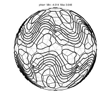
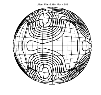
Figure 6: Geopotential error ($\mathrm{m}^{2}\mathrm{s}^{-2}$) after 5 days for the solid body rotation test case. Left: hexagonal mesh, 10242 cells. Right: cubed sphere mesh, 13824 cells. In each case 11 evenly space contours (i.e. 10 intervals) are used between the minimum and maximum values. (The coarse resolution meshes shown as background are for orientation only.)

5.4 Flow over an isolated mountain

Test case 5 of Williamson et al. (1992) involves an initial solid body rotation flow impinging on a conical mid-latitude mountain, leading to the generation of gravity and Rossby waves and, eventually, a complex nonlinear flow. There is no analytical solution for this test case, so a high-resolution reference solution was generated using the semi-implict, semi-Lagrangian ENDGame shallow water model (Zerroukat et al., 2009). The finite element model runs stably with the time steps given in table 3, but, as discussed by Thuburn et al. (2014) for the finite volume model and for ENDGame itself, the errors are then dominated by the semi-implicit treatment of the large amplitude gravity waves present in the solution. At any given resolution, the errors look almost identical for all combinations of model and mesh tested. The test was therefore repeated with the time steps reduced by a factor 4. The resulting height errors at day 15 are shown in table 4. The errors on the two meshes are generally very similar, and in most cases are a little smaller than those produced by the finite volume model (Thuburn et al., 2014, table 7).

Table 4: Height errors ($\mathrm{m}$) for test case 5.

Ncells	$\Delta t\ \ \mathrm{(s)}$	$L_{1}(h)$	$L_{2}(h)$	$L_{\infty}(h)$
Hex
642	1800	36.37	50.91	191.47
2562	900	11.62	15.83	66.84
10242	450	3.12	4.11	15.06
40962	225	1.27	1.82	9.28
Cube
864	1800	44.11	64.93	291.35
3456	900	17.57	25.14	100.66
13824	450	3.75	5.25	21.42
55296	225	1.08	1.46	6.47

Maps of height error at day 15 are shown in Fig. 7. The errors produced by the finite element model are of comparable size to those from ENDGame, though the error patterns are different in the three cases. Comparison with figure 6 of Thuburn et al. (2014) confirms that the errors in the finite element model are somewhat smaller than those in the finite volume model.

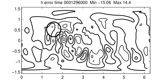
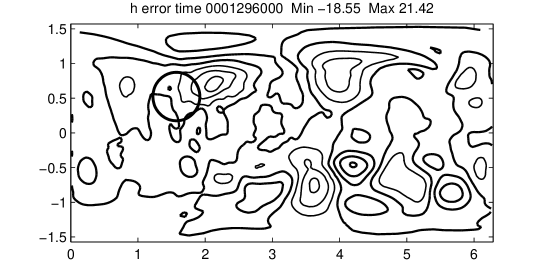
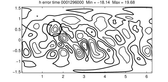
Figure 7: Height errors ($\mathrm{m}$) at day 15 for the isolated mountain test case. Top: hexagonal mesh, 10242 cells. Middle: cubed sphere mesh, 13824 cells. Bottom: ENDGame on a regular longitude-latitude mesh, $160\times 80$ cells. The contour interval is $6\,\mathrm{m}$, and zero and negative contours are bold. The bold circle indicates the position of the mountain.

This test case was also run to 50 days at the highest resolutions in table 4 and several diagnostics relevant to the mimetic properties of the scheme were calculated. The results are very similar to those shown in figure 8 of Thuburn et al. (2014). They confirm that mass is conserved to within roundoff error, and that changes in the total available energy (available potential energy plus kinetic energy) are much smaller than the conversions between available potential energy and kinetic energy. The dissipation of available energy and potential enstrophy is associated almost entirely with the inherent scale-selective dissipation in the advection scheme; it is very small, of order 1 part per thousand, during the first 20 days, but increases subsequently as PV contours begin to wrap up and nonlinear cascades become significant, implying that the inherent dissipation adapts automatically to the flow complexity in a reasonable way. A dual-mass-like tracer remains consistent with the diagnosed dual mass field $\bar{\phi}$ to within $2$ parts in $10^{4}$, and a PV-like tracer remains consistent with the diagnosed PV field, to within $3$ parts in $10^{3}$. The small errors result from imperfect convergence of various iterative aspects of the solver, and can be reduced by taking more iterations.

5.5 Barotropically unstable jet

The test case proposed by Galewsky et al. (2004) follows the evolution of a perturbed barotropically unstable jet. The case tests the ability of models to handle the complex small scale vorticity features produced by the rapidly growing instability. The results are very sensitive to spurious triggering of the instability by error patterns related to the mesh structure.

Figure 8 shows the relative vorticity field at day 6 for the hexagonal mesh with 10242 cells and 163842 cells, the cubed sphere mesh with 13824 cells and 221184 cells, and, for comparison, from ENDGame on a $640\times 320$ longitude-latitude mesh. In all cases the vorticity field is free of noise and spurious ripples. However, at coarse resolution the finite element model solutions show distinct ‘grid imprinting’, with a zonal wavenumber 5 pattern on the hexagonal mesh and a zonal wavenumber 4 pattern on the cubed sphere mesh. At finer resolution the solutions are more similar to the ENDGame solution, but still show significant development in the longitude range $\pi/2$ to $\pi$ where the jet in the ENDGame solution remains quiescent. The solutions on the hexagonal mesh, especially at the finer resolution, are remarkably similar to those from the finite volume model (Thuburn et al., 2014, figure 9). On the other hand, the solutions on the cubed sphere mesh show some noticable differences from the finite volume model. At the finer resolution, outside the region strongly affected by the spurious devleopment, the structure of vorticity features is slightly more accurate in the finite element model.

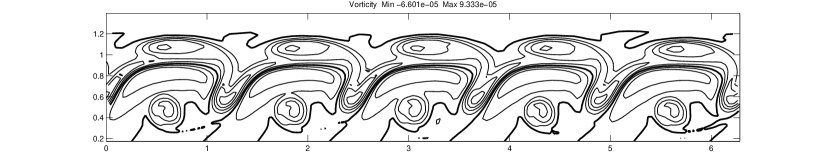
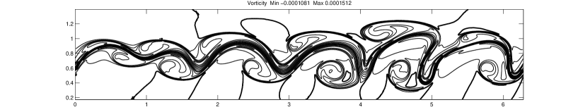
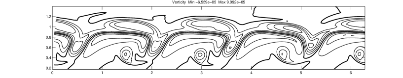
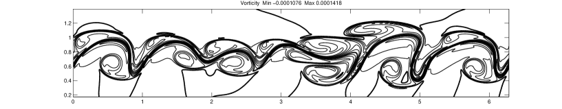
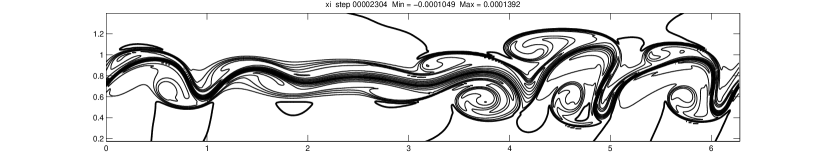
Figure 8: Relative vorticity field at day 6 for the barotropic instability test case. Row 1: hexagonal mesh, 10242 cells, $\Delta t=900\,\mathrm{s}$. Row 2: hexagonal mesh, 163842 cells, $\Delta t=225\,\mathrm{s}$. Row 3: cubed sphere mesh, 13824 cells, $\Delta t=900\,\mathrm{s}$. Row 4: cubed sphere mesh, 221184 cells, $\Delta t=225\,\mathrm{s}$. Row 5: ENDGame, $640\times 320$ cells, $\Delta t=225\,\mathrm{s}$. The plotted region is $0^{\mathrm{o}}$ to $360^{\mathrm{o}}$ longitude, $10^{\mathrm{o}}$ to $80^{\mathrm{o}}$ latitude. The contour interval is $2\times 10^{-5}\,\mathrm{s}^{-1}$.

6 Conclusions and discussion

A method of constructing low-order mimetic finite element spaces on arbitrary two-dimensional polygonal meshes, using compound elements, has been presented, along with corresponding discrete Hodge star operators for mapping between primal and dual function spaces. The method has been used as the basis of a numerical model to solve the shallow water equations on a rotating sphere. The model has the same mimetic properties, which underpin the ability to capture important physical properties, as the finite volume model of Thuburn et al. (2014), but with improved accuracy.

The finite volume model of Thuburn et al. (2014) relies on certain properties of the mesh for accuracy, namely the Heikes and Randall (1995b) optimization on the hexagonal mesh and the placement of primal vertices relative to dual vertices on the cubed sphere mesh. Although identical meshes have been used here to ensure the cleanest possible comparison, the mimetic finite element scheme does not depend on such mesh properties for accuracy; thus it provides greater flexibility in the choice of mesh.

An important practical consideration is the computational cost of the method. As a rough guide, the cost of the finite element model on a single processor varied between 3.3 and 4.6 times the cost of ENDGame for the cubed sphere mesh and between 4.2 and 7.3 times the cost of ENDGame for the hexagonal mesh, at the resolutions tested. (For comparison, the cost of the finite volume model varied between 2.7 and 3.7 times the cost of ENDGame for the cubed sphere mesh and between 3.3 and 4.9 times the cost of ENDGame for the hexagonal mesh.) The greater cost on the hexagonal mesh compared to the cubed sphere results from a combination of a greater stencil size for some operators and, in the current implementation, a less cache-friendly mesh numbering (the latter could straightfowardly be optimized). Given the potential to optimize the implementation and the expected gains in parallel scalability from the quasi-uniform mesh, these figures suggest that, despite the need for indirect addressing and the need to invert several linear operators, the finite element method need not be prohibitively expensive compared to methods currently used for operational forecasting, typified by ENDGame.

Computing integrals over compound elements is more complex and costly than for the usual triangular or quadrilateral elements. In the current implementation, all the operators $L$, $M$, $H$, $J$, $R$, $W$, and $T$ are precomputed, thus avoiding the need for any run-time quadrature in the finite element parts of the calculations. (Also, once these operators are computed, there is no need to retain the details of how the compound elements were built from subelements.) This precomputation is possible because all but one of these operators are linear; the only nonlinear term (other than advection) is a simple quadratic nonlinearity in the kinetic energy. In a system with more complex nonlinearities, such as the pressure gradient term in a compressible three-dimensional fluid, precomputation might not be possible and some run time quadrature would be unavoidable. Even so, in a high performance computing environment it is not clear whether precomputation or run-time quadrature would be most efficient, given the relative cost of memory access and computation (David Ham, pers. comm.).

The mathematical similarity of the finite element and finite volume formulations has been emphasized, the principal difference being the appearance of mass matrices in the finite element formulation. The similarity is made even clearer if we use (51), (52) and (80) to rewrite (94) in the equivalent dual space form

$$\dot{\hat{U}}+\widehat{Q^{\perp}}+\overline{D}_{1}(\hat{\Phi}+\hat{K})=0.$$ (117)

The velocity degrees of freedom then correspond to dual edge circulations, and $\hat{U}$ can be identified with the $V$ of Thuburn et al. (2014). Equations (93) and (117) explicitly involve only the topological derivative operators $D_{2}$ and $\overline{D}_{1}$; the metric enters through the Hodge star operators needed to map between primal and dual function spaces. This approach of isolating the metric from the purely topological operators in order to construct numerical methods with mimetic properties on complex geometries or meshes has been advocated by several authors (e.g. Bossavit, 1998; Hiptmair, 2001; Palha et al., 2014, and references therein).

It is also worth emphasizing that the roles of primal and dual function spaces are not symmetrical here. Although any given field may be represented in both the primal and dual spaces, with a reversible Hodge star map between them, only primal space test functions are ever used, and so only primal space mass matrices appear, and dual space weak derivatives are never needed. (An interesting alternative would be to use only dual space test functions; then the prognostic equations remain (93) and (117), but (51)-(53) are replaced by

$$I^{T}\Phi=\hat{L}\hat{\Phi},$$ (118)

$$H^{T}U=\hat{M}\hat{U},$$ (119)

$$J^{T}\Xi=\hat{N}\hat{\Xi},$$ (120)

where $\hat{L}$, $\hat{M}$ and $\hat{N}$ are the mass matrices for the spaces $\mathbf{V}^{0}$, $\mathbf{V}^{1}$ and $\mathbf{V}^{2}$, respectively.)

Only the lowest order polygonal finite element spaces are used here: compound $\text{P1-RT0-P0}^{\text{DG}}$. An interesting question is whether the approach can be extended to higher order. The harmonic extension idea of Christiansen (2008) has been extended to higher order by Christiansen (2010). It appears plausible that higher order compound elements could be built from constrained linear combinations of, for example, the $\text{P2}^{+}\text{-BDFM1-P1}^{\text{DG}}$ elements recommended by Cotter and Shipton (2012), but the details have yet to be worked out. A more subtle question is whether suitable higher order dual spaces can be constructed.

Another, more straightforward, extension of the compound element approach is to three dimensions. The compound elements used here can be extruded into polygonal prisms; we have made some initial progress in working out the details of using such a scheme for the compressible Euler equations. (In atmosphere and ocean models it is desirable, for several reasons, to use a columnar mesh.) Fully three-dimensional compound elements can also be constructed using the discrete harmonic extension approach. These might be useful, for example, to implement a finite element version of the cut cell method for handling bottom topography (e.g. Lock et al., 2012, and references therein) while retaining a columnar mesh.

Besides their ability to use arbitrary polygonal meshes, another potentially useful property of the compound elements used here is that the function spaces are built directly in physical space, without the need for Piola transforms. Thus, for example, globally constant functions are always contained in $\mathbf{V}_{2}$. In this way, the compound elements avoid the reduced convergence rate, and even loss of consistency, discussed by Arnold et al. (2014), and so provide an alternative to the rehabilitation technique of Bochev and Ridzal (2008).

Acknowledgements

We are grateful to Thomas Dubos for drawing our attention to the work of Buffa and Christiansen (2007) and Christiansen (2008), to Martin Schreiber and David Ham for valuable discussions on code optimization, and to Nigel Wood for helpful comments on a draft of this paper. This work was funded by the Natural Environment Research Council under the “Gung Ho” project (grants NE/I021136/1, NE/I02013X/1, NE/K006762/1 and NE/K006789/1).

Appendix A Operator inverses and sparse approximate $M$ inverse

Inverses of the $H$ and $J$ operators are needed at the beginning of every time step, and inverses of $H$ and $M$ are needed at every Newton iteration. These are computed by (under- or over-relaxed) Jacobi iteration based on a diagonal approximation of the relevant operator. E.g., to solve $Ax=R$, define

$$x^{(1)}=(A^{*})^{-1}R$$ (121)

where $A^{*}$ is a diagonal approximation to $A$, then iterate:

$$x^{(l+1)}=x^{(l)}+\mu(A^{*})^{-1}(R-Ax^{(l)}).$$ (122)

A diagonal approximation $J^{*}$ to the operator $J$ is defined by demanding that, for every dual cell $j$, $J^{*}$ and $J$ should give the same result in dual cell $j$ when acting on the $\mathbf{V}^{2}$ representation of a constant scalar field. A diagonal approximation $M^{*}$ to the velocity mass matrix $M$ is defined by demanding that, for every edge $e$, $M^{*}$ and $M$ should give the same result at edge $e$ when acting on the $\mathbf{V}_{1}$ representation of a solid body rotation velocity field whose maximum velocity is normal to primal edge $e$. A diagonal approximation $H^{*}$ to the operator $H$ is defined by demanding that, for every edge $e$, $H^{*}$ and $H$ should give the same result at edge $e$ when acting on the $\mathbf{V}^{1}$ representation of a solid body rotation velocity field whose maximum velocity is tangential to dual edge $e$.

Optimal values of the relaxation parameter $\mu$ were found to depend on the operator and mesh structure. The values used are given in table 5.

Table 5: Relaxation parameters used for Jacobi iteration for operator inverses.

Grid	$J^{-1}$	$M^{-1}$	$H^{-1}$
Hex	1.4	1.4	1.4
Cube	1.4	0.9	1.4

For the inverses that occur once per time step, 10 Jacobi iterations are used. For those that occur at every Newton iteration, 2 Jacobi iterations are used taking the solution obtained at the previous Newton iteration as the first guess (or (121) on the first Newton iteration).

A sparse approximate inverse $\mathcal{M}^{-1}$ of the $\mathbf{V}_{1}$ mass matrix is needed for the Helmholtz problem. On the hexagonal mesh it is sufficient to use a diagonal approximation

$$\mathcal{M}^{-1}=(M^{*})^{-1}.$$ (123)

However, on the cubed sphere mesh, whose dual and primal edges are not mutually orthogonal, such a diagonal approximation is less accurate and limits the convergence of the Newton iterations. Therefore we use instead an approximation based on a single Jacobi iteration towards the inverse of $M$:

$$\mathcal{M}^{-1}=(M^{*})^{-1}\left\{(1+\mu)\mathrm{Id}-\mu M(M^{*})^{-1}\right\},$$ (124)

where $\mathrm{Id}$ is the identity matrix. This approximate inverse is not diagonal but has the same stencil as $M$ itself.

References

References

- Arnold et al. (2014) Arnold, D. N., Boffi, D. and Bonizzoni, F.: Finite element differential forms on curvilinear cubic meshes and their approximation properties, Numer. Math., DOI:10.1007/s00211-014-0631-3, 2014.
- Bochev and Ridzal (2008) Rehabilitation of the lowest-order Raviart-Thomas element on quadrilateral grids, SIAM J. Numer. Anal., 47, 487–507, 2008.
- Bossavit (1998) Bossavit, A.: Computational Electromagnetism: Variational Formulation, Complementarity, Edge Elements. Academic Press Electromagnetism Series, Number 2 San Diego: Academic Press, 1998.
- Buffa and Christiansen (2007) Buffa, A., and Christiansen, S. H.: A dual finite element complex on the barycentric refinement, Math. of Comput., 76, 1743–1769, 2007.
- Christiansen (2008) Christiansen, S. H.: A construction of spaces of compatible differential forms on cellular complexes, Math. Models and Methods in Appl. Sci., 18, 739–757, 2008.
- Christiansen (2010) Christiansen, S. H.: Minimal mixed finite elements on polyhedra, C. R. Acad. Sci. Paris, 348, 217–221, 2010.