Radio-Gamma-ray connection and spectral evolution in 4C +49.22 (S4 1150+49): the Fermi, Swift and Planck view

Abstract

The Large Area Telescope on board the Fermi Gamma-ray Space Telescope detected a strong $\gamma$-ray flare on 2011 May 15 from a source identified as 4C +49.22, a flat spectrum radio quasar also known as S4 1150+49. This blazar, characterised by a prominent radio-optical-X-ray jet, was in a low $\gamma$-ray activity state during the first years of Fermi observations. Simultaneous observations during the quiescent, outburst and post-flare $\gamma$-ray states were obtained by Swift, Planck and optical-IR-radio telescopes (INAOE, Catalina CSS, VLBA, Metsähovi). The flare is observed from microwave to X-ray bands with correlated variability and the Fermi, Swift and Planck data for this FSRQ show some features more typical of BL Lac objects, like the synchrotron peak in the optical band that outshines the thermal blue-bump emission, and the X-ray spectral softening. Multi-epoch VLBA observations show the ejection of a new component close in time with the GeV $\gamma$-ray flare. The radio-to-gamma-ray spectral energy distribution is modeled and fitted successfully for the outburst and the post-flare epochs using either a single flaring blob with two emission processes (synchrotron self Compton, and external-radiation Compton), and a two-zone model with SSC-only mechanism.

  

1 Introduction

Data and results from simultaneous and coordinated $\gamma$-ray and multi-wavelength (MW) observations of the flat spectrum radio quasar (FSRQ) 4C +49.22 (also known as S4 1150+49, OM 484, SBS 1150+497 and GB1 1150+497), are presented.

4C +49.22 is a core-dominated, radio-loud FSRQ located at $z=0.334$ (Lynds & Wills, 1968; Burbidge, 1968; Stepanian et al., 2001). The Sloan Digital Sky Survey (SDSS; Adelman-McCarthy et al., 2008) DR7 and DR8 give values of $z=0.3339$ and of $z=0.33364$, respectively. This blazar shows a kiloparsec-extent and one-sided, knotty and wiggling radio jet, with high surface brightness, sharp bends and resolved substructures (see, e.g., Owen & Puschell, 1984; Akujor & Garrington, 1991; Sambruna et al., 2004, 2006a, 2006b). The jet, known to show constant low optical polarisation (Moore & Stockman, 1981), has a twisted morphology with a corkscrew structure reminiscent of 3C 273 and, remarkably, is also well detected at X-ray and optical bands. The 10$\arcsec$ X-ray jet of 4C +49.22  is one of the brightest known among blazars, and is an example of X-ray emission produced by inverse Compton (IC) scattering of the cosmic microwave background (CMB) photons (Tavecchio et al., 2005; Hardcastle, 2006; Sambruna et al., 2006a).

The Chandra X-ray Observatory detected a Fe K-shell emission line in 4C +49.22  consistent with fluorescent $K\alpha$ emission from cold iron (Gambill et al., 2003; Sambruna et al., 2006a, b). The estimated mass of the super-massive black hole (SMBH) is $3.3\times 10^{8}M_{\odot}$ according to the FWHM of the broad $H\beta$ line (4810 km s^-1; Shields et al., 2003) and is $1.6\times 10^{9}M_{\odot}$ according to the estimation from the host galaxy luminosity (Decarli et al., 2008). From the SDSS R5 spectrum the continuum luminosity of the Broad Line Region (BLR) at 5100 Å  is evaluated to be $\ F_{\lambda}=10^{44.6}$ erg s^-1 with a BLR size of $R_{BLR}=1.26\times 10^{17}$ cm (Decarli et al., 2008).

4C +49.22 showed a large $\gamma$-ray outburst detected with the Large Area Telescope onboard the Fermi Gamma-ray Space Telescope (Fermi-LAT), at energies above 100 MeV on 2011 May 15 (Reyes et al., 2011). Before this flaring event the source was in a long-standing quiescent state with no detection reported in the first Fermi-LAT source catalogue (Abdo et al., 2010b) or in previous source catalogs released by other MeV-GeV $\gamma$-ray missions like EGRET (Hartman et al., 1999) and AGILE (Pittori et al., 2009). It was included in the second Fermi-LAT source catalogue (Nolan et al., 2012, 2FGL hereafter; 2FGL J1153.2+4935) with a 2-year averaged $\gamma$-ray flux ($E>100$ MeV) of ($2.6\pm 0.4$) $\times 10^{-8}$ photons cm^-2 s^-1. During the flare the source reached a flux almost two orders of magnitude higher than the 2FGL average flux. The source was significantly detected on a daily timescale in 2011 April (Hays & Donato, 2011). The $\gamma$-ray spectrum did not show significant changes during the outburst compared to the pre and post-flare days. In the post-flare phase Swift-XRT reported an X-ray flux six times higher than previous archival XRT observations (Reyes et al., 2011). This FSRQ was also observed with the Planck satellite. According to the Planck-On-the-Fly Forecaster, 4C +49.22 was observed by Planck from 2011 May 11 to May 26. We exploited Planck, Swift and Fermi simultaneous data, for the first time, to study this blazar. We collected Spectral Energy Distribution (SED) archival data from several surveys and telescopes, from radio to $\gamma$ rays: Dixon Master List of Radio Sources (Dixon, 1970); the FIRST Survey Catalog of 1.4-GHz Radio Sources (White et al., 1997); Kuehr Extragalactic Radio Sources at 5 GHz (Kuehr et al., 1981); the NRAO VLA Sky Survey (Condon et al., 1998); the VLA Low-Frequency Sky Survey at 74 MHz (Cohen et al., 2007); the Green Bank 6-cm Catalog of Radio Sources (Gregory et al., 1997); the 20-cm Northern Sky Catalog; the Planck Early Release Compact Source Catalogue (Planck Collaboration et al., 2011); Five-Year Wilkinson Microwave Anisotropy Probe (Wright et al., 2009); the SDSS; the ROSAT All-Sky Survey Bright Source Catalogue (Voges et al., 1999), the ROSAT Catalog of PSPC WGA Sources (White et al., 1994); and the 2FGL catalog.

The paper is organised as follows. In Section 2 the Fermi-LAT data analysis is presented, while in Section 3 the millimetre Planck data from the sky coverages with Planck are described, with particular attention to the fourth sky scan that is coincident in time with the 2011 May $\gamma$-ray outburst. In Section 4 optical, UV and X-ray data from nine Swift pointings under the Target of Opportunity programme (ToO) performed between 2011 April 26 and May 25 are presented. Section 5 reports on ground-based radio-to-optical observations obtained by the VLBA (MOJAVE monitoring programme) and Metsähovi radio observatories, and by near-IR and optical photometric observations of the INAOE observatory and the Catalina Sky Survey (CSS). Section 6 characterises the $\gamma$-ray variability and cross correlations in 4C +49.22 through 3 years of Fermi-LAT survey data, with particular focus on the outburst of 2011 May. Multi-epoch SEDs are built for the source and modeled with a one-zone with two components Synchrotron Self-Compton (SSC) and External Radiation Compton (ERC) description and a two-zone Synchrotron Self-Compton description in Section 7. This allows us to infer both the production sites of the high-energy emission and emission scenarios. A summary and conclusions are reported in Section 8. We adopted a standard spatially-flat six-parameter $\Lambda$ cold dark matter ($\Lambda$-CDM) cosmology based on Planck results (Ade et al., 2013), namely with $\Omega_{m}$=0.315 and $H_{0}$= 67.3 km s^-1 Mpc^-1. The corresponding luminosity distance at $z=0.334$ is $d_{L}$= 1822.3 Mpc.

2 $\gamma$-ray observations and analysis of FERMI-LAT data

The LAT instrument is a pair conversion telescope comprising a modular array of 16 towers—each with a tracker module of silicon micro-strip detectors and a hodoscopic calorimeter of CsI(Tl) crystals—surrounded by an Anti-Coincidence Detector made of tiles of plastic scintillator. The LAT is capable of measuring the directions and energies of $\gamma$-ray photons with energies from 20 MeV to $>300$ GeV (for details, see, Atwood et al., 2009; Abdo et al., 2009b; Ackermann et al., 2012).

The data presented in this paper were collected in the first three years of Fermi science observations, from 2008 August 4 to 2011 August 4 (MJD 54682-55778) with E $>$ 100 MeV. Photon events were selected using the Pass 7 event classification and reconstruction and the corresponding Instrument Response Functions (IRFs) P7SOURCE_V6. This selection provides a clean set of events (in terms of direction, energy reconstruction and background rejection) a large effective area and well understood response functions for point source analysis. To minimise contamination from photons produced by cosmic rays interacting with the Earth’s atmosphere, $\gamma$-ray events that have reconstructed directions with angles $>100^{\circ}$ with respect to the local zenith have been excluded and the time intervals when the rocking angle of the LAT was greater than $52^{\circ}$ were rejected.

The reduction and analysis of LAT data was performed using the ScienceTools v09r23p01, specifically using an unbinned maximum-likelihood estimator of the spectral model parameters (gtlike tool). For 4C +49.22, which is located at high Galactic latitude, events are extracted within a $10^{\circ}$ radius of the region of interest (ROI) centred at the position of the radio source counterpart. This angular radius, comparable to the 68% containment angle of the Point Spread Function (PSF) at the lowest energies, provides sufficient events to accurately constrain the diffuse emission components. Following the 2FGL catalogue the spectral model used for 4C +49.22 is the power-law flux density distribution of the form $F(E)=N_{0}(E/E_{0})^{-\Gamma}$. The source region model includes all point sources in the 2FGL within $20^{\circ}$ of 4C +49.22 (source region) including 4C +49.22 itself. The sources within the $10^{\circ}$ radius of ROI were fitted with a power-law flux density distribution with photon indices $\Gamma$ frozen to the values obtained from the likelihood analysis of the full data set, while those beyond $10^{\circ}$ ROI radius had both index $\Gamma$ and normalisation frozen to those found in the 2FGL catalogue.

A Galactic diffuse emission model (gal_2yearp7v6_v0.fits) and Isotropic component (iso_p7v6source.txt) were used to model the background.

For the light curve extraction, which is presented in Section 6, the Upper Limits (UL) at 2-$\sigma$ confidence level were computed for time intervals in which the likelihood Test Statistic (TS; Mattox et al., 1996) was less than 9 or the number of model predicted $\gamma$ rays for 4C +49.22 $N_{pred}<3$ or $\Delta F(E)/F(E)>0.5$. The UL estimation procedures are described in the 2FGL catalogue paper (Nolan et al., 2012).

Details on the unbinned likelihood spectra fit for 4C +49.22 in the 0.1-100 GeV range are reported in Table 1 and SED data points for both epochs are reported in Table 2. The estimated systematic uncertainty of the integral fluxes above 100 MeV is about 8.1% and -6.9% for a soft source like 4C +49.22 (Ackermann et al., 2012); the stated uncertainties in the fluxes are statistical only.

Table 1: Summary of the unbinned likelihood spectral fit above 100 MeV

Interval	Best-fit Model and Parameters
Integrated data	Power-law
2008-08-08 (MJD: 54686)	$\Gamma=2.26\pm 0.04$
2011-08-04 (MJD: 55777)	F${}_{E>100~{}\mathrm{MeV}}$ = (5.8$\pm$ 0.3)$\times 10^{-8}$ [ph cm-2 s-1]
Outburst/high state	Power-law
2011-05-14 (MJD: 55695)	$\Gamma=2.20\pm 0.09$
2011-05-16 (MJD: 55697)	F${}_{E>100~{}\mathrm{MeV}}$ = (1.5$\pm$ 0.2)$\times 10^{-6}$ [ph cm-2 s-1]
Post-flare/lower state	Power-law
2011-05-17 (MJD: 55698)	$\Gamma=2.23\pm 0.08$
2011-05-26 (MJD: 55707)	F${}_{E>100~{}\mathrm{MeV}}$ = (6.4$\pm$ 0.6)$\times 10^{-7}$ [ph cm-2 s-1]

3 Simultaneous mm observations and results by Planck

Planck (Tauber et al., 2010; Planck Collaboration et al., 2011, 2013) is the third generation space mission to measure the anisotropy of the cosmic microwave background. It observes the sky in nine frequency bands covering 30–857 GHz with high sensitivity and angular resolution from 31^′ to 5^′. Full sky coverage is attained in $\sim$ 7 months. The Low Frequency Instrument (LFI; Mandolesi et al. 2010; Zacchei et al. 2011; Planck Collaboration et al. 2013) covers the 30, 44 and 70 GHz bands with amplifiers cooled to 20 K. The High Frequency Instrument (HFI; Planck HFI Core Team et al. 2011; Planck Collaboration et al. 2013) covers the 100, 143, 217, 353, 545 and 857 GHz bands with bolometers cooled to 0.1 K. Polarisation is measured in all but the highest two bands (Leahy et al., 2010; Rosset et al., 2010). A combination of radiative cooling and three mechanical coolers produces the temperatures needed for the detectors and optics (Planck Collaboration et al., 2011). Two Data Processing Centers (DPCs) check and calibrate the data and make maps of the sky (Planck HFI Core Team et al., 2011; Zacchei et al., 2011). Planck’s sensitivity, angular resolution, and frequency coverage make it a powerful instrument for Galactic and extragalactic astrophysics as well as cosmology. The Planck beams scan the entire sky exactly twice in one year, but scan only about 95 % of the sky in six months. For convenience, we call an approximately six month period a “survey”, and use it as a shorthand for one coverage of the sky. In order to take advantage of the simultaneity between the Planck observations and the Fermi-LAT $\gamma$-ray flare of 2011 May 15, flux densities have been extracted from maps produced using only data collected during a portion of the Planck fourth sky survey (2011 May 11-26). Moreover, for comparison we have also extracted flux densities from separate maps for the first (2009 November 16-26), the second (2010 May 11-26) and the third Planck survey (2010 November 16-26). Results are reported in Table LABEL:tab:planckdata. The Early Release Compact Source catalogue (ERCSC, Planck Collaboration et al. 2011) and the Planck catalogue of Compact Sources (PCCS, Planck Collaboration et al. 2013) include average flux densities for 4C +49.22. All of these maps have been produced through the standard LFI and HFI pipelines adopted for the internal DX8 release. LFI flux densities were obtained at 30, 44 and 70 GHz using the IFCAMEX code, an implementation of the Mexican Hat Wavelet 2 (MHW2) algorithm that is being used in the LFI DPC infrastructure to detect and extract flux densities of point-like sources in CMB maps. This wavelet is defined as the fourth derivative of the two-dimensional Gaussian function, where the scale of the filter is optimized to look for the maximum in the S/N of the sources in the filtered map, and has been previously applied to WMAP and Planck data and simulations (González-Nuevo et al., 2006; López-Caniego et al., 2006, 2007; Massardi et al., 2009). First, we obtained a flat patch centred on the source and applied the MHW2 software. This algorithm produces an unbiased estimation of the flux density of the source and its error. Second, we convert the peak flux density from temperature units to Jy/sr and then to Jy by multiplying it by the area of the instrument beam, taking the beam solid angle into account. In this analysis we used the effective Gaussian full width at half maximum (FWHM) whose area is that of the actual elliptical beam at 30, 44 and 70 GHz, respectively, as provided by the LFI DPC. HFI flux densities have been extracted using aperture photometry. Flux densities were evaluated assuming a circularly symmetric Gaussian beam of the given FWHM. An aperture is centred on the position of the source and an annulus around this aperture is used to evaluate the background. A correction factor which accounts for the flux of the source in the annulus may be calculated and is given below, where $k_{0}$, $k_{1}$ and $k_{2}$ are the number of FWHMs of the radius of the aperture, the inner radius of the annulus and the outer radius of the annulus respectively.

$$\tiny F_{true}=\left(1-\left(\frac{1}{2}\right)^{4k_{0}^{2}}-\left(\left(\frac{1}{2}\right)^{4k_{1}^{2}}-\left(\frac{1}{2}\right)^{4k_{2}^{2}}\right)\frac{k_{0}^{2}}{k_{2}^{2}-k_{1}^{2}}\right)^{-1}F_{obs}$$ (1)

Here we used a radius of 1 FWHM for the aperture, $k_{0}=1$; the annulus is located immediately outside of the aperture and has a width of 1 FWHM, $k_{1}=1$ and $k_{2}=2$. The flux density, $F_{true}$ may then be evaluated from the observed flux density, $F_{obs}$, where $F_{obs}$ is the total flux inside the aperture after the background has been subtracted. Planck data for each survey are reported in Table LABEL:tab:planckdata.

Table 2: Fermi-LAT spectral energy distribution data points

Epoch	frequency	$\nu~{}f(\nu)$
	[Hz]	[erg cm-2 s-1]
2011-05-15	(6.0$\pm$0.3)$\times 10^{22}$	(2.5$\pm$0.3)$\times 10^{-10}$
(MJD: 55696)	(2.4$\pm$0.3)$\times 10^{23}$	(2.2$\pm$0.3)$\times 10^{-10}$
	(9.5$\pm$0.3)$\times 10^{23}$	(1.4$\pm$0.4)$\times 10^{-10}$
	(3.8$\pm$0.3)$\times 10^{24}$	(8.3$\pm$5.9)$\times 10^{-11}$
2011-05-17/25	(6.0$\pm$0.3)$\times 10^{22}$	(1.1$\pm$0.1)$\times 10^{-10}$
(MJD: 556978/55706)	(2.4$\pm$0.3)$\times 10^{23}$	(8.6$\pm$1.3)$\times 10^{-11}$
	(9.5$\pm$0.3)$\times 10^{23}$	(6.4$\pm$1.7)$\times 10^{-11}$
	(3.8$\pm$0.3)$\times 10^{24}$	(4.9$\pm$2.8)$\times 10^{-11}$

Table 3: Flux densities for 4C +49.22 from the four Planck surveys. First survey: 2009 November 16-26, second survey: 2010 May 11-26, third survey: 2010 November 16-26, fourth survey: 2011 May 11-26.

Planck-LFI	$\nu$	Flux Density	Errors
survey	[GHz]	[Jy]	[Jy]
1st	30	1.14	0.15
2nd	30	1.66	0.12
3rd	30	1.75	0.14
4th	30	1.46	0.13
1st	44	1.24	0.26
2nd	44	1.93	0.24
3rd	44	1.28	0.26
4th	44	1.95	0.13
1st	70	1.21	0.13
2nd	70	1.85	0.18
3rd	70	1.40	0.23
4th	70	2.36	0.16
Planck-HFI	$\nu$	Flux Density	Errors
survey	[GHz]	[Jy]	[Jy]
1st	100	0.57	0.23
2nd	100	1.93	0.15
3rd	100	1.58	0.17
4th	100	2.37	0.17
1st	143	0.51	0.20
2nd	143	1.62	0.16
3rd	143	1.58	0.18
4th	143	2.26	0.15
1st	217	0.41	0.10
2nd	217	1.48	0.11
3rd	217	1.30	0.08
4th	217	1.98	0.09
1st	353	0.42	0.20
2nd	353	0.98	0.09
3rd	353	1.04	0.12
4th	353	1.61	0.09
1st	545	0.20	0.21
2nd	545	0.76	0.17
3rd	545	0.72	0.18
4th	545	1.34	0.20
1st	857	0.25	UL
2nd	857	0.17	0.23
3rd	857	0.32	0.27
4th	857	0.74	0.20

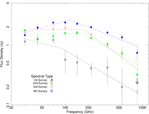
Figure 1: Planck flux densities for 4C +49.22 at all nine frequencies as reported in Table LABEL:tab:planckdata. Each frequency is shown in four colours corresponding to four surveys: black open circles correspond to the first survey, red open squares to the second, green filled squares to the third and blue filled circle to the fourth.

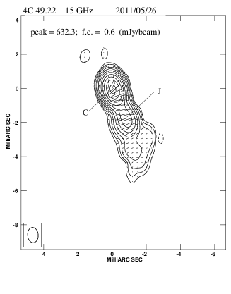
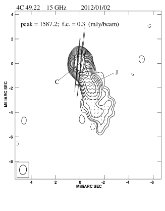
Figure 3: 15-GHz VLBA images of 4C +49.22  from the observations in 2011 May (upper panel) and 2012 January (bottom panel). On each image, we provide the observing date. The peak flux density is in mJy/beam and the first contour (f.c.) intensity is in mJy/beam, which corresponds to three times the off-source noise level. Contour levels increase by a factor of 2. The restoring beam is plotted in the bottom left-hand corner. The vectors superimposed on the total intensity flux density contours show the position angle of the electric vector, where 1 mm length corresponds to 7.1 mJy/beam.

Spectra presented in Figure 1 are modeled with a broken power-law; see Equation 5 of León-Tavares et al. (2012), in order to characterise the evolution of the sub-mm spectra in terms of the spectral classification presented in Figure 3 of León-Tavares et al. (2012). Within the mentioned classification scheme the hard sub-mm spectrum observed during 2009 November (open circles) can be classified as spectral-type A (both power-law indices, $\alpha_{mm}<0$ , $\alpha_{sub-mm}<0$ and the relative difference between indices is less than 50%), thus indicating the absence of a new jet component in a very early development stage. As the plasma blob propagates down the jet, the shape of the spectrum changes; the relative difference between $\alpha_{mm}$ and $\alpha_{sub-mm}$ became greater than 50% as can be seen in 2010 May and 2010 November, respectively. These spectral shapes can be classified as spectral-type C. As the plasma blob propagates down the jet, its spectral turnover shifts to lower frequencies, from 170 GHz of 2010 May and 2010 November to around 100 GHz in 2011 May. The sub-mm spectrum of 2011 May, simultaneous to the $\gamma$-ray flare, shows a well-defined synchrotron component and it is consistent with spectral-type D ($\alpha_{mm}>0$ and $\alpha_{sub-mm}<0$). Sources with sub-mm spectra classified as spectral type C or D are more likely to be strong $\gamma$-ray emitters, which is in good agreement with the fact that 4C +49.22 became a $\gamma$-ray emitter only after its sub-mm spectral shape changed to spectral-type D (León-Tavares et al., 2012). This spectral shape can be associated with a single synchrotron component that becomes self absorbed in the middle of the mm wavelength regime. Such high spectral turnover frequencies reveal the presence of emerging disturbances in the jet that are likely to be responsible for the high levels of $\gamma$-ray emission (Marscher, 2006, 2014).

4 Simultaneous X-ray and UV-optical observations and results from Swift

Table 4: Log and fitting results of the data obtained by the XRT instrument on board Swift.

Date	Exp. Time	Photon Index	Unabsorbed Flux 0.3–10 keV	$\chi 2_{\rm red}$ (d.o.f.)
	(s)		erg cm-2 s-1
2008-04-28 (MJD: 54584)	5438	1.82 $\pm$ 0.11	(4.8 $\pm$ 0.4)$\times$10-12	0.83 (24)
2009-05-06 (MJD: 54957)	3122	1.80 $\pm$ 0.16	(3.8 $\pm$ 0.5)$\times$10-12	0.64 (10)
2009-11-17 (MJD: 55152)	5218	2.05 $\pm$ 0.14	(3.8 $\pm$ 0.4)$\times$10-12	0.71 (17)
2011-04-26 (MJD: 55677)	4647	1.99 $\pm$ 0.08	(1.1 $\pm$ 0.1)$\times$10-11	0.75 (44)
2011-04-29 (MJD: 55680)	4813	1.69 $\pm$ 0.10	(7.8 $\pm$ 0.6)$\times$10-12	0.91 (32)
2011-05-02 (MJD: 55683)	4396	1.77 $\pm$ 0.11	(7.6 $\pm$ 0.6)$\times$10-12	1.10 (27)
2011-05-15 (MJD: 55696)	3611	2.03 $\pm$ 0.06	(2.1 $\pm$ 0.1)$\times$10-11	0.79 (77)
2011-05-17 (MJD: 55698)	3406	1.70 $\pm$ 0.08	(1.2 $\pm$ 0.1)$\times$10-11	0.75 (36)
2011-05-19 (MJD: 55700)	3708	1.87 $\pm$ 0.08	(1.2 $\pm$ 0.1)$\times$10-11	0.92 (42)
2011-05-22 (MJD: 55703)	4141	1.74 $\pm$ 0.09	(8.4 $\pm$ 0.6)$\times$10-12	0.73 (32)
2011-05-23 (MJD: 55704)	4002	1.69 $\pm$ 0.09	(9.3 $\pm$ 0.7)$\times$10-12	0.86 (31)
2011-05-25 (MJD: 55706)	3920	1.70 $\pm$ 0.10	(8.8 $\pm$ 0.7)$\times$10-12	1.03 (31)
2011-05-17/25 (MJD: 55698/55706)	19176	1.76 $\pm$ 0.04	(1.1 $\pm$ 0.1)$\times$10-11	0.93 (152)

In response to the high $\gamma$-ray activity of 4C +49.22, the Swift satellite (Gehrels et al., 2004) performed 9 ToO observations, between 2011 April 26 and May 25. In order to reference the source’s past activity, we also analysed the observations performed on 2008 April 8, 2009 May 6, and 2009 May 17. The 2011 observations were performed using two of three on-board instruments: the X-ray Telescope (XRT; Burrows et al., 2005, 0.2–10.0 keV) and the UltraViolet Optical Telescope (UVOT; Roming et al., 2005, 170–600 nm). The archival data from the Burst Alert Telescope (BAT; Barthelmy et al., 2005, 15–150 keV) from Cusumano et al. (2010a) and Cusumano et al. (2010b) were added to the SEDs as reference of the low state.

The XRT data were reprocessed with standard procedures (xrtpipeline v0.12.6), filtering and screening criteria by using the Heasoft package (v6.10). We considered data collected using the photon counting (PC) mode with XRT event grades between 0 and 12. Since the source count rate was always below 0.5 counts s^-1 no pile-up correction was necessary. Source events were extracted from a circular region with a radius of 20 pixels (1 pixel $\sim$ 2.36$\arcsec$), while background events were extracted from a circular region with a radius of 50 pixels, away from background sources. Ancillary response files were generated with xrtmkarf, and account for different extraction regions, vignetting and PSF corrections. We used the spectral redistribution matrices v011 in the calibration database maintained by HEASARC.

All spectra were rebinned with a minimum of 20 counts per energy bin to allow $\chi^{2}$ fitting within XSPEC (v12.6.0). We fit the individual spectra with a simple absorbed power-law, with a neutral hydrogen column fixed to its Galactic value (2.13$\times$10²⁰ cm^-2; Kalberla et al. 2005). In addition, we summed the data collected after the $\gamma$-ray flare (2011 May 17-25) in order to have better statistics see SED figures in Section 7. The fit results are reported in Table 4 and the SED data points are reported in Table 5. During the 9 ToOs performed in 2011 April-May, Swift-XRT observed a 0.3–10 keV flux in the range (0.8-2.1) $\times$ 10^-11 erg cm^-2 s^-1, a factor between 2 and 5 higher than the flux level observed in 2008–2009. This is an hint that the mechanism that produced an increase of the activity observed in $\gamma$-rays also affected the X-ray part of the spectrum.

The peak of the X-ray flux was detected on 2011 May 15, soon after the major $\gamma$-ray flare was detected by Fermi-LAT. The flare X-ray spectrum was softer than that of the post-flare epoch, thus demonstrating the contribution of the synchrotron component to lower energy X-ray emission. This implies a shift of the synchrotron and IC peaks toward higher energies on May 15.

Figure 2: Photometric U-band intra-day light curve obtained by Swift-UVOT in 2011 May 15.

The Swift-UVOT can acquire images in six lenticular filters (V, B, U, UVW1, UVM2 and UVW2, with central wavelengths in the range 170–600 nm). After seven years of operations, observations are now carried out using only one of the filters unless specifically requested by the user. Therefore, images are not always available for all filters in all the observations. The log of Swift-UVOT observations analysed is reported in Table 6.

The photometry analysis of all the 4C +49.22 observations was performed using the standard UVOT software distributed within the HEAsoft 6.9.0 package and the calibration included in the most recent release of the “Calibration Database”.

We extracted source counts using a standard circular aperture with a 5″ radius for all filters, and the background counts using an annular aperture with an inner radius of 26″  and a width of 8″. Source counts were converted to fluxes using the task uvotsource and the standard zero points (Poole et al., 2008). Fluxes were then de-reddened using the appropriate values of $E(B-V)$ for the source taken from Schlegel et al. (1998) and the $A_{\lambda}/E(B-V)$ ratios calculated for UVOT filters using the mean Galactic interstellar extinction curve from Fitzpatrick (1999).

Using U-band filter images only, we detected variability within a single exposure (a few hours timescale) in the flare observation of 2011 May 15. We show in Figure 2 the U-band flux variation within this observation. If we compare the first “segment” of the exposure to the last, the variation is about 7$\sigma$. This last segment is the shortest (34 s), and has the largest flux error. Intra-day variability in a single observation has been detected also on May 19 in U, and on May 22 in M2 filters. The May 19 observation includes three segments and shows a flux increase on the last one (1230 s), while on May 22 the third (191 s) of four segments shows a lower flux. The May 19 episode is the most significant, with a $\sim$10$\sigma$ variation.

Table 5: Swift-XRT spectral energy distribution data points

Epoch	frequency	$\nu~{}f(\nu)$
	[Hz]	[erg cm-2 s-1]
2011-05-15	9.1$\times$1016	(6.5$\pm$0.4)$\times$10-12
(MJD: 55696)	1.4$\times$1017	(6.1$\pm$0.4)$\times$10-12
	1.9$\times$1017	(6.8$\pm$0.4)$\times$10-12
	2.5$\times$1017	(6.0$\pm$0.4)$\times$10-12
	3.2$\times$1017	(6.9$\pm$0.5)$\times$10-12
	3.9$\times$1017	(5.9$\pm$0.4)$\times$10-12
	5.6$\times$1017	(6.4$\pm$0.4)$\times$10-12
	9.5$\times$1017	(6.3$\pm$0.4)$\times$10-12
	1.6$\times$1018	(6.5$\pm$1.5)$\times$10-12
2011-05-17/25	8.8$\times$1016	(2.1$\pm$0.1)$\times$10-12
(MJD: 55698/55706)	1.3$\times$1017	(2.2$\pm$0.1)$\times$10-12
	1.7$\times$1017	(2.4$\pm$0.1)$\times$10-12
	2.1$\times$1017	(2.5$\pm$0.1)$\times$10-12
	2.5$\times$1017	(2.8$\pm$0.2)$\times$10-12
	2.9$\times$1017	(2.7$\pm$0.1)$\times$10-12
	3.4$\times$1017	(2.8$\pm$0.1)$\times$10-12
	4.1$\times$1017	(3.0$\pm$0.2)$\times$10-12
	4.9$\times$1017	(3.1$\pm$0.2)$\times$10-12
	6.1$\times$1017	(3.3$\pm$0.2)$\times$10-12
	7.8$\times$1017	(3.7$\pm$0.2)$\times$10-12
	1.0$\times$1018	(3.9$\pm$0.2)$\times$10-12
	1.5$\times$1017	(4.1$\pm$0.3)$\times$10-12

5 Ground based and longer term radio-optical observations

5.1 MOJAVE monitoring and component motion studies

In order to study the parsec-scale morphology and possible changes in the source structure, we analysed 13-epoch VLBA observations at 15 GHz from the MOJAVE programme spanning a time interval from 2008 May to 2013 February. We imported the calibrated uv data sets (Lister et al., 2009) into the NRAO AIPS package and performed a few phase-only self-calibration iterations before producing the final total intensity images. Uncertainties on the flux density scale are within 5% (Lister et al., 2013). For the six data sets obtained after the $\gamma$-ray flare we also produced Stokes’ Q and U images to study possible variations of the source polarisation. The uncertainties on the polarisation angle are less than 5^∘ (Lister et al., 2013).

The source 4C +49.22 shows a one-sided core-jet structure that is 6 mas in size (i.e. $\sim$28 pc at the source redshift) and the radio emission is dominated by the core component, labeled C in Figure 3. Following a detection of the $\gamma$-ray flare on 2011 May 15, the core component of this source showed an increase in both the total intensity of emission and the polarisation percentage, while the polarisation angle has rotated by about 60^∘. On the other hand, no significant changes have been found in the jet structure, labeled J in Figure 3, strongly suggesting that the region responsible for the radio variability is located within the central component. Total intensity flux density and polarisation properties of the core and jet components are reported in Table 7.

The total intensity and polarisation flux densities were measured on the image plane with the Astronomical Image Processing System (AIPS) using the Gaussian-profile fitting task JMFIT and the task TVSTAT, which performs an aperture integration on a selected region. As the source core we consider the unresolved central component, and we derive its parameters with JMFIT. The jet is the remaining structure, and the parameters are obtained by subtracting the core contribution to the total emission measured by TVSTAT. Errors are computed using the formulas from Fanti et al. (2001).

To derive structural changes, in addition to the analysis performed on the image plane, we also fitted the visibility data with circular Gaussian components at each epoch using the model-fitting option in DIFMAP. Errors $\Delta r$ associated with the component position are estimated by means of $\Delta r=a/(S_{\rm p}/rms)$, where $a$ is the component deconvolved major-axis, $S_{\rm p}$ is its peak flux density and rms is the 1$\sigma$ noise level measured on the image plane (Orienti et al., 2011). In case the errors estimated are unreliably small, we assume a more conservative value for $\Delta r$ that is 10% of the beam.

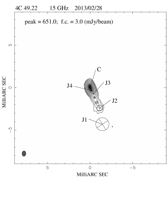
Figure 4: 15-GHz VLBA image from the observations performed during 2013 February with the positions of the of the jet components discussed in Section 5.1. The peak flux density is in mJy/beam and the first contour (f.c.) intensity is in mJy/beam, and it corresponds to 0.5 % of the peak flux density. Contour levels increase by a factor of 2. The restoring beam is plotted in the bottom left-hand corner.

This approach is preferable in order to derive small variations in the source structure; it also provides a more accurate fit of unresolved structures close to the core component. Throughout the observing epochs we could reliably follow the motion of only two components, labeled J1 and J2 in Figure 4; a third component, J3, became visible in the last seven epochs. Interestingly, a new component, J4, was detected in the last three epochs of MOJAVE data, since 2012 August. We determined the separation velocity from the core, considered stationary, for these four components by means of a linear regression fit that minimises the chi-square error statistics (Figure 5). From this analysis we found that J1, J2, J3 and J4 are increasing their separation from the core with apparent angular velocities of 0.48$\pm$0.01, 0.27$\pm$0.01, 0.30$\pm$0.02 and 0.27$\pm$0.09 mas/yr, which correspond to apparent linear velocities $\beta_{\rm app}=v_{app}/c$ of 9.9$\pm$0.2, 5.6$\pm$0.2, 6.2$\pm$0.4, and 5.6$\pm$1.4, respectively. The velocity derived for J1 is in agreement with the value found by Lister et al. (2013), while for J2 we obtain a slower speed. This may be due to a deceleration that may become detectable with the availability of additional observing epochs not considered in Lister et al. (2013). The large uncertainty on the velocity of component J4 is due to the availability of only 3 observing epochs spanning a very short time interval of about 7 months. From a linear regression fit we estimated the time of zero separation, which provides an indication of the ejection epoch. We found that J4 emerged from the core on 2011.52 (i.e., beginning of July 2011), making the ejection of the component close in time to the $\gamma$-ray flare. However, the large uncertainties on the separation velocity do not allow us to accurately constrain the precise time of zero separation, which ranges between 2010.73 (i.e. 2010 September) and 2011.92 (i.e. 2011 December). It is worth noting that the time of zero separation estimated for component J3 is 2010.3$\pm$0.2 (i.e. 2010 April) with an associated uncertainty on the ejection time that ranges between 2010 February and June. Interestingly, no strong $\gamma$-ray flare was reported close in time with the ejection of this component, but the source turned out to be repeatedly detectable by LAT on a weekly time scale after 2010 February (see Section 6). By means of the apparent velocities derived for the jet components, we estimated the possible combination of the intrinsic velocity $\beta=v/c$ and the angle $\theta$ that the jet forms with our line of sight:

$$\beta_{\rm app}=\frac{\beta{\rm sin}\theta}{1-\beta{\rm cos}\theta}$$ (2)

We assumed that $\beta_{\rm app}$ is between 9.9 and 5.6, i.e. the velocity estimated for the fastest and slowest components. In the former case we found that $\beta>0.995$ and $\theta<11^{\circ}$, while in the latter $\beta>0.985$ and $\theta<20^{\circ}$. Another way to derive the possible ($\beta$-$\theta$) combinations is using the flux density ratio of the approaching, $S_{\rm a}$, and receding $S_{\rm r}$ jets:

$$\frac{S_{\rm a}}{S_{\rm r}}=\left(\frac{1+\beta{\rm cos}\theta}{1-\beta{\rm cos}\theta}\right)^{3+\alpha}$$ (3)

where $\alpha$ is the spectral index ($S_{\nu}\propto\nu^{-\alpha}$), and it is assumed to be 0.7, i.e. a typical value for the jet component. From the lack of detection of a counterjet in any of the images, we set a lower limit on the jet/counterjet ratio. We used the highest ratio between the jet and counterjet emission, which is computed by using $S_{\rm a}=816$ mJy (i.e. the flux density of J4 as it emerges from the core, see Table 7), and $S_{\rm r}=0.3$ mJy, which corresponds to 1$\sigma$ rms. From these values we derive a jet/counterjet ratio $>$2720. This value yields $\beta$cos$\theta>$0.79 c, implying $\beta>0.79$ and $\theta<38^{\circ}$, which are consistent with the range found from Equation 2.

With the derived values we can compute a lower limit on the Doppler factor by means of:

$$\mathcal{D}=\frac{1}{\Gamma(1-\beta{\rm cos}\theta)}$$ (4)

where $\Gamma$ is the bulk Lorentz factor. The lower limit on the Doppler factor is $\mathcal{D}>4.2$, which is compatible with those derived from our SED modeling (see Section 7). However, this estimate is affected by the large uncertainties in the apparent velocity and more observations spanning a larger time interval with frequent time sampling are necessary. Our SED modeling results (Section 7) are constrained to $\mathcal{D}$ values between $\sim$20 and $\sim$30, maintaining therefore the agreement with variability Doppler factors obtained recently for a sample of Fermi-LAT blazars (e.g., Pushkarev et al., 2009; Savolainen et al., 2010), and in particular maintaining the agreement with previous SED modeling of 4C +49.22 (Sambruna et al., 2006b). The observed increasing flux density and polarisation degree in the radio core of 4C +49.22 after the GeV $\gamma$-ray flare demonstrate that the high-energy peak emission is produced in or close to the radio core rather than in structures and blobs at larger distance along the jet, far from the central engine.

Even if this does not yet constrain the flaring GeV emission region (sometimes called the “blazar zone”) to within the BLR, we can at least exclude flaring GeV emission produced by jet knots placed at a large distance from the central engine (e.g., few parsecs Lister et al., 2013). This result can help to discriminate between our multi-temporal and multi-wavelength SED modeling described in Section 7.

Table 6: Log of the data obtained by the UVOT instrument on board Swift. All magnitudes are corrected for Galactic extinction.

Date	Exp. Time	V	B	U	W1	M2	W2
	(s)	(Mag)	(Mag)	(Mag)	(Mag)	(Mag)	(Mag)
2008-04-28 (MJD: 54584)	5398	–	–	–	15.64$\pm$0.04	–	–
2009-05-06 (MJD: 54957)	2980	17.62$\pm$0.09	17.59$\pm$0.05	16.40$\pm$0.04	16.42$\pm$0.05	15.91$\pm$0.05	16.06$\pm$0.04
2009-11-17 (MJD: 55152)	5034	17.34$\pm$0.07	17.18$\pm$0.04	16.01$\pm$0.03	15.72$\pm$0.04	15.28$\pm$0.04	15.41$\pm$0.03
2011-04-26 (MJD: 55677)	1336	–	–	–	14.77$\pm$0.04	–	–
2011-04-29 (MJD: 55680)	4750	16.37$\pm$0.04	16.55$\pm$0.04	15.55$\pm$0.04	15.42$\pm$0.04	15.10$\pm$0.04	15.22$\pm$0.04
2011-05-02 (MJD: 55683)	4247	15.97$\pm$0.04	16.27$\pm$0.04	15.21$\pm$0.04	15.12$\pm$0.04	14.82$\pm$0.04	14.96$\pm$0.04
2011-05-15 (MJD: 55696)	3592	–	–	14.14$\pm$0.02	–	–	–
2011-05-17 (MJD: 55698)	3390	15.50$\pm$0.03	15.70$\pm$0.02	14.79$\pm$0.02	14.73$\pm$0.03	14.56$\pm$0.04	14.70$\pm$0.03
2011-05-19 (MJD: 55700)	3689	–	–	14.25$\pm$0.02	–	–	–
2011-05-22 (MJD: 55703)	4077	–	–	–	15.14$\pm$0.03	14.87$\pm$0.03	15.04$\pm$0.03
2011-05-23 (MJD: 55704)	3936	–	–	–	14.70$\pm$0.03	14.47$\pm$0.03	14.63$\pm$0.03
2011-05-25 (MJD: 55706)	3849	–	–	–	15.28$\pm$0.03	14.97$\pm$0.03	15.15$\pm$0.03

Table 7: Total intensity flux density and polarisation properties. Column 1: observing date; Cols. 2, and 3: total intensity flux density of component C and J, respectively; Cols. 4, and 5: polarised flux density (and polarisation percentage) for component C and J, respectively; Cols. 6, and 7: polarisation angle for component C and J, respectively.

Date	$S_{\rm C}$	$S_{\rm J}$	$S_{\rm pol,C}$	$S_{\rm pol,J}$	$\chi_{\rm C}$	$\chi_{\rm J}$
	mJy	mJy	mJy (%)	mJy (%)	deg	deg
2011-05-26 (MJD: 55707)	658$\pm$33	88$\pm$5	5.8$\pm$0.5 (0.9$\pm$0.1%)	7.2$\pm$0.7 (8.1$\pm$0.8%)	-64$\pm$5	-66$\pm$5
2011-08-15 (MJD: 55788)	947$\pm$47	91$\pm$5	9.4$\pm$0.6 (1.0$\pm$0.1%)	7.4$\pm$0.7 (8.1$\pm$0.8%)	-84$\pm$5	-77$\pm$5
2012-01-02 (MJD: 55928)	1708$\pm$85	87$\pm$4	45.1$\pm$2.2 (2.6$\pm$0.1%)	8.2$\pm$0.8 (9.4$\pm$0.8%)	-10$\pm$5	-73$\pm$5
2012-08-03 (MJD: 56142)	1650$\pm$82	92$\pm$5	59.0$\pm$3.0 (3.5$\pm$0.2%)	6.0$\pm$0.7 (6.5$\pm$0.7%)	10$\pm$5	-62$\pm$5
2012-11-11 (MJD: 56242)	1381$\pm$69	63$\pm$3	62.0$\pm$3.1 (4.5$\pm$0.2%)	5.0$\pm$0.6 (7.9$\pm$0.9%)	19$\pm$5	-67$\pm$5
2013-02-28 (MJD: 56351)	1081$\pm$54	65$\pm$3	20.0$\pm$1.1 (1.9$\pm$0.1%)	6.0$\pm$0.7 (9.2$\pm$1.0%)	48$\pm$5	-70$\pm$5

Figure 5: Changes in separation with time between component C, considered stationary, and J1, J2, J3 and J4. The solid lines represent the linear fits to the data, while the dotted lines represent the uncertainties from the fit parameters. The vertical dashed line indicates the time of the $\gamma$-ray flare.

5.2 Metsähovi Radio Observatory

Observations at 37 GHz were made with the 13.7 m diameter Metsähovi radio telescope, which is a radome-enclosed paraboloid antenna situated in Finland. The measurements were made with a 1 GHz-band dual beam receiver centred at 36.8 GHz. The observations are ON–ON observations, alternating the source and the sky in each feed horn. A typical integration time to obtain one flux density data point is between 1200 and 1400 s. The detection limit of the telescope at 37 GHz is on the order of 0.2 Jy under optimal conditions. Data points with a signal-to-noise ratio $<$ 4 are handled as non-detections. The flux density scale is set by observations of DR 21. Sources NGC 7027, M 87 (3C 274) and NGC 1275 (Per A, 3C 84) are used as secondary calibrators. A detailed description of the data reduction and analysis is given in Teräsranta et al. (1998). The error estimate in the flux density includes the contribution from the measurement rms and the uncertainty of the absolute calibration. The flux density light curve is shown in Figure 6 and Table LABEL:tab:mets.

Table 8: Flux densities of 4C +49.22 with Metsähovi Radio Observator at 37 GHz

Date	Flux Density
	[mJy]
2008-08-06 (MJD: 54684.0)	0.90$\pm$0.08
2009-01-03 (MJD: 54834.0)	1.12$\pm$0.09
2009-02-10 (MJD: 54872.0)	0.90$\pm$0.12
2009-04-23 (MJD: 54944.0)	1.10$\pm$0.09
2009-09-20 (MJD: 55094.0)	0.63$\pm$0.11
2009-11-12 (MJD: 55147.0)	0.90$\pm$0.13
2009-11-30 (MJD: 55165.0)	1.25$\pm$0.11
2009-12-12 (MJD: 55177.0)	0.81$\pm$0.11
2010-02-25 (MJD: 55252.0)	1.54$\pm$0.1
2010-05-12 (MJD: 55328.0)	1.41$\pm$0.13
2010-05-25 (MJD: 55341.0)	1.27$\pm$0.09
2010-06-27 (MJD: 55374.0)	1.92$\pm$0.11
2010-11-07 (MJD: 55507.0)	1.94$\pm$0.3
2011-02-03 (MJD: 55595.0)	1.14$\pm$0.1
2011-02-06 (MJD: 55598.0)	1.03$\pm$0.14
2011-03-18 (MJD: 55638.0)	1.26$\pm$0.11
2011-05-18 (MJD: 55699.0)	1.45$\pm$0.14
2011-05-22 (MJD: 55703.0)	1.71$\pm$0.09
2011-05-26 (MJD: 55707.0)	1.57$\pm$0.17
2011-05-27 (MJD: 55708.0)	1.46$\pm$0.1
2011-05-28 (MJD: 55709.0)	1.61$\pm$0.19
2011-05-29 (MJD: 55710.0)	1.42$\pm$0.08
2011-05-30 (MJD: 55711.0)	1.52$\pm$0.14
2011-06-01 (MJD: 55713.0)	1.22$\pm$0.09
2011-06-02 (MJD: 55714.0)	1.61$\pm$0.09
2011-06-05 (MJD: 55717.0)	1.53$\pm$0.09
2011-07-24 (MJD: 55766.0)	1.91$\pm$0.28
2011-08-10 (MJD: 55783.0)	2.07$\pm$0.09

5.3 Quasi-Simultaneous near-infrared monitoring by INAOE

The Near-infrared (NIR) photometry was performed in J, $K_{s}$ and H band with the CANICA NIR camera at the 2.1-m telescope of the Observatorio Astrofísico Guillermo Haro (OAGH) in Cananea, Sonora, Mexico. CANICA is a camera based on a HAWAII 1024 $\times$ 1024 pixel array, with plate scale and field of view 0.32 ″ pixel^-1 and about 5.5 $\times$ 5.5 square arcmin, respectively. Observations were reduced using standard differential aperture photometry with IRAF packages. Every night, several standard stars from Hunt et al. (1998) were observed in both bands. The photometric error for each night was assumed to be the standard deviation between our estimated magnitude and the magnitude determined in Hunt et al. (1998) for the standard stars observed. The mean zero-point error in J and H in the photometric nights is 0.06 mag, reaching 0.08 mag on the photometric nights. Similarly, in $K_{s}$ we have errors of 0.08 and 0.10 mag, respectively. As expected, the error estimates show that the photometric accuracy is generally higher in J and H than in $K_{s}$. We note that our average errors in the photometric zero-point are 0.07 mag in J and H and 0.09 mag in $K_{s}$, which is quite good for NIR bands. The flux densities in the three filters are reported in Figure 7 and in Table LABEL:tab:inaoe.

Each image was checked for problems before going through all the data-reduction steps. For the treatment of the images, we used the GEMINI IRAF1 package. Flat-field images were obtained through the QFLAT task from combining many dome images. We decided to use dome flat-fields instead of flat images obtained from sky images; after checking with many standard stars, we discovered that the former produced more accurate results in terms of photometry (i.e. smaller zero-point errors). The QSKY task was used to estimate the background contribution. For each image, the background was estimated from the four sky images closest in time. Furthermore, the mean and standard deviation of each sky image were calculated, and if the mean was discrepant from that of the other three sky images by more than 10 % of the standard deviation then the image was removed from the process. In this way, we avoid background changes and ensure a proper background subtraction. These corrections (flat-fielding and background subtraction) were performed for every galaxy and standard star image by QREDUCE, using the appropriate flat-field and background images. Finally, the IMCOADD task combines all corrected images of a galaxy according to their median, calculating the necessary shifts due to the dither pattern.

Table 9: Magnitudes and flux densities of 4C +49.22 with INAOE Telescope

Filters	Date	Magnitude	flux
			[mJy]
J	2011-04-29 (MJD: 55680.84)	14.45$\pm$0.07	2.66$\pm$0.32
	2011-05-09 (MJD: 55690.78)	14.55$\pm$0.07	2.41$\pm$0.29
	2011-05-10 (MJD: 55691.77)	14.29$\pm$0.07	3.06$\pm$0.37
	2011-05-14 (MJD: 55695.75)	13.33$\pm$0.07	7.46$\pm$0.92
	2011-05-21 (MJD: 55702.77)	13.42$\pm$0.07	6.83$\pm$0.84
	2011-05-23 (MJD: 55704.69)	13.63$\pm$0.09	5.62$\pm$0.89
	2011-05-24 (MJD: 55705.74)	13.68$\pm$0.05	5.40$\pm$0.47
H	2011-04-29 (MJD: 55680.82)	13.50$\pm$0.08	4.26$\pm$0.90
	2011-05-09 (MJD: 55690.78)	13.80$\pm$0.09	3.24$\pm$0.77
	2011-05-10 (MJD: 55691.76)	13.42$\pm$0.08	4.56$\pm$0.96
	2011-05-13 (MJD: 55694.77)	13.04$\pm$0.08	6.51$\pm$1.37
	2011-05-14 (MJD: 55695.75)	12.49$\pm$0.07	10.8$\pm$1.99
	2011-05-21 (MJD: 55702.76)	12.40$\pm$0.07	11.7$\pm$2.16
	2011-05-23 (MJD: 55704.69)	12.76$\pm$0.06	8.44$\pm$1.33
	2011-05-24 (MJD: 55705.74)	12.89$\pm$0.06	7.46$\pm$1.18
Ks	2011-04-29 (MJD: 55680.85)	12.50$\pm$0.11	6.61$\pm$3.09
	2011-05-09 (MJD: 55690.79)	12.73$\pm$0.06	5.37$\pm$1.37
	2011-05-10 (MJD: 55691.78)	12.62$\pm$0.12	5.95$\pm$3.03
	2011-05-14 (MJD: 55695.75)	11.53$\pm$0.12	16.2$\pm$8.30
	2011-05-21 (MJD: 55702.78)	11.86$\pm$0.12	12.0$\pm$6.12
	2011-05-23 (MJD: 55704.69)	12.07$\pm$0.12	9.91$\pm$5.05
	2011-05-24 (MJD: 55705.74)	12.13$\pm$0.09	9.36$\pm$3.58

5.4 Catalina Sky Survey observations

The Catalina Sky Survey for near-Earth objects and potential planetary hazard asteroids (NEO/PHA) is conducted by the University of Arizona Lunar and Planetary Laboratory group. CSS utilizes three wide-field telescopes: the 0.68-m Catalina Schmidt at Catalina Station, AZ; the 0.5-m Uppsala Schmidt (Siding Spring Survey, or SSS, in collaboration with the Australian National University) at Siding Spring Observatory, NSW, Australia; and the Mt. Lemmon Survey (MLS), a 1.5-m reflector located on Mt. Lemmon, AZ. Each telescope employs a camera with a single, cooled, 4k$\times$4k back-illuminated, unfiltered CCD. Between the three telescopes, the majority of the observable sky is covered at least once (and up to 4 times) per lunation, depending on the time since the area was last surveyed and its proximity to the ecliptic. The total area coverage is $\sim$ 30,000 deg², and it excludes the Galactic plane within $|b|<10^{\circ}$. For each coverage four images of the same field are taken, separated in time by $\sim$ 10 min, for a total time baseline of $\sim$ 30 min in that sequence. Typically 2 to 4 such sequences are obtained per field per lunation; the cycle is generally repeated the next lunation, marching through the RA range during the year. The time baselines now extend to 6 years with up to $\sim$ 300 exposures per pointing over much of the area surveyed so far. This represents an unprecedented coverage in terms of the combined area, depth, and number of epochs. The photometric flux data of 4C +49.22 are retrieved through the Catalina Surveys Data Release services (see Figure 6).

6 $\gamma$-ray flare and time variability

To investigate the behaviour of this source, in particular the flaring state phase, we extracted the light curves from the entire data set using different time binnings (1 week, 3 days and 1 day time bins) with gtlike. The source spectrum was fitted with a power-law function. In the case of 1 day time bins, we fixed the photon index to the value found in the whole energy band, integrating over 3 years of data. For longer time bins the photon index was left free to vary. The lowest panel of Figure 6 shows the whole Fermi-LAT lightcurve with a weekly time bins. We report in the same figure radio and optical long-term observations by Metsähovi and Planck and Catalina Sky Survey. Figure 7 shows the parts of the multi-frequency light curves during the main flaring activity, increasing in frequency from the top to the bottom panel. We studied the evolution of spectral shape during the flaring state for the X-ray and $\gamma$-ray components. We show in Figure 7 the photon index values versus time with overlayed Fermi-LAT lightcurve shape in the inset panels. We performed a linear regression to evaluate the dependence between flux values and spectral indices, for Fermi-LAT no spectral evolution is evident during the flaring state with a regression coeffient of $r\sim 0.01$, but for the X-rays, a softer when brighter behaviour consistent with a shift in the synchrotron peak during the flaring state is noticeable ($r\sim 0.74$).

A direct comparison of the Fermi-LAT and CSS light curves clearly shows that an optical brightening occurred at the time of the $\gamma$-ray flare. Since no optical data for the same filter are available for the post-flare relaxing phase we cannot estimate any time lag. Although the Swift-XRT data only cover a limited time range (see Figure 7) these observations suggest a strong correlation between the X-ray and GeV flux. This correlation is illustrated in Figure 8 where we have plotted the $\gamma$-ray versus X-ray flux at the times of the X-ray Swift-XRT measurements. During the period of the last Swift-XRT observation the source was not detected by Fermi-LAT and we did also include the upper limit in Figure 8. The $\gamma$-ray flux for each point was obtained by linear interpolation of the 1-day bin LAT light curve. With only 9 X-ray points available a standard discrete cross correlation function (DCCF) would be very poorly sampled. On timescales longer than the flare lengths of a few days the DCCF contains no significant information. It is however possible to use the DCCF on shorter timescales to estimate a time lag between the X-ray and $\gamma$-ray variations. In Figure 9 we show the DCCF for lags less than 3 days computed by oversampling the 1 day binned LAT light curve by a factor of 19, to give a larger oversampling, before correlating it with the X-ray points. The Gaussian fit, which is also shown in the figure, gives an estimated time lag $\Delta t=-0.4\pm 1.0$ days (where negative lag means X-rays preceding $\gamma$-rays). Uncertainty estimates were made by two different Monte Carlo methods: the model independent approach by Peterson et al. (1998) and by simulated flare light curves. In the second approach double sided exponential flares were sampled in a similar manner to the observations in order to investigate uncertainties due to the precise timing of the X-ray observations. The two methods gave consistent estimates.

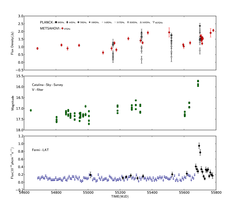
Figure 6: Multi-frequency light curves using the long term monitoring data. Top panel: Metsähovi radio data and Planck (described in Sect. 5.2 and in Sect. 3), middle panel: Catalina Sky Survey (described in Sect. 5.4), bottom panel: 36 months $\gamma$-ray integrated flux ($E>100$ MeV) lightcurve measured by Fermi-LAT from 2008 August 4 to 2011 August 4. The time binning is 7 days: blue arrows represent the 2-$\sigma$ upper limits (described in Sect. 2).

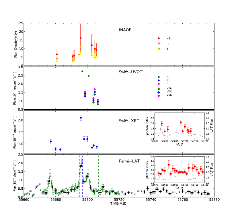
Figure 7: Multi-frequency light curves zoomed in to the main flaring period (2011 May). In the first panel INAOE data points are shown in the different filters (described in Sect. 5.3); in the second panel, Swift-UVOT (described in Sect. 4); in the third panel, Swift-XRT (described in Sect. 4); and in the fourth panel, Fermi-LAT 1 day time bin data, are shown (described in Sect. 2). The blue and green dashed lines represent the two states considered in the SED modeling. The inset panels report the spectral indices coming from the power-law spectral fit in each bin with superimposed the Fermi-LAT $\gamma$-ray lightcurve.

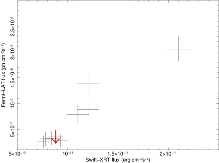
Figure 8: $\gamma$-ray vs. X-ray flux at the times of Swift-XRT observations. Fermi-LAT fluxes were interpolated from the 1 day binned $\gamma$-ray light curve.

Figure 9: Discrete Cross Correlation Function using the Swift-XRT data and the Fermi-LAT 1 day binned $\gamma$-ray lightcurve, The dashed curve is a Gaussian fit to the DCCF peak. The time lag is estimated to be $-0.4\pm 1.0$ days (negative means X-rays leading $\gamma$-rays).

We analysed the $\gamma$-ray flare of 2011 May 15 (MJD 55696), using the following function $F(t)$, already proposed in Abdo et al. (2010a), to fit the $\gamma$-ray light curve shape during each single flare:

$$F(t)=F_{c}+F_{0}\left(e^{\frac{t_{0}-t}{T_{r}}}+e^{\frac{t-t_{0}}{T_{d}}}\right)^{-1}$$ (5)

Here, $F_{c}$ represents the baseline of the flux lightcurve, $F_{0}$ measures the amplitude of the flares, $t_{0}$ describes approximatively the time of the peak (it corresponds to the actual maximum only for symmetric flares), $T_{r}$ and $T_{d}$ the time of the rise and decay of each flare, respectively. Figure 10 shows the light curve for the main flaring period that occurred in 2011 May, with the fit function superimposed. In Table LABEL:fit_par we reported the fit parameter value. Using this technique it is also possible to estimate the shortest time variability (to be conservative, the shortest value extracted is $\Delta t=2T_{r}=0.33$ days), which is used to put an important constraint on the radiative region size $R_{rad}\leq(c\Delta t\mathcal{D})/(1+z)$, where c is the speed of light, $\mathcal{D}=1/(\Gamma(1-\beta cos\theta))$ is the Doppler beaming factor, $\Gamma$ the bulk Lorentz factor, $\theta$ the viewing angle and $z$ the cosmological redshift. Using the Doppler factors obtained from the SED fitting procedure, which are in agreement with blazars with strong $\gamma$-ray emission (Savolainen et al., 2010), we can estimate that $R_{rad}$ is $\lesssim 2.5\times 10^{16}$ cm for $\mathcal{D}=20$ and $\lesssim 3.8\times 10^{16}$ cm for $\mathcal{D}=30$.

Table 10: Parameter values extracted from the flare shape fit.

$t_{max}$	$T_{r}\pm err$	$T_{d}\pm err$
$(MJD)$	(day)	(day)
55676.2	0.33 $\pm$ 0.07	0.81 $\pm$ 0.15
55696.3	1.69 $\pm$ 0.24	0.29 $\pm$ 0.05
55700.4	1.96 $\pm$ 0.34	0.54 $\pm$ 0.11

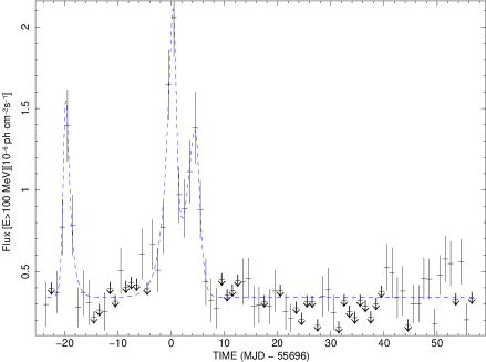
Figure 10: One day time bin light curve of Fermi-LAT data zoomed in to the flaring period of 2011 May with superimposed fitting function shown as a blue dashed line.

7 Radio-to-gamma-ray Spectral Energy Distribution

Variability is a powerful diagnostic for the physics of blazars but creates difficulties in the broad-band SED analysis because theoretical models can be effectively constrained only with sufficiently-well time resolved multi-frequency data. For example Fermi-driven observing campaigns are demonstrating the role of SSC emission for FSRQ objects (Böttcher et al., 2009), while the ERC process is being used in fitting also the SEDs of BL Lac objects. First clues, suggesting a smooth transition between the division of blazars into BL Lac objects and FSRQs, are emerging in some studies (e.g., Cavaliere & D’Elia, 2002; Giommi et al., 2012b; Sbarrato et al., 2012). Our Fermi, Swift and Planck results on the FSRQ 4C +49.22 are pointing out some features more typical of BL Lac objects, and therefore support this hypothesis.

The big blue bump (thermal disc emission) in 4C +49.22 appears clearly in the low emission state SED (see Figures 11 and 12), which is based on archival data; however, it is completely overwhelmed by the continuous synchrotron emission during the $\gamma$-ray flaring state. The lack of observable thermal disc emission is a common feature in BL Lac objects, for which contribution from the accretion disc is negligible in both low and high activity states.

The SED of 4C +49.22 obtained during two epochs, flare and post-flare, through Fermi, Swift, Planck and radio-optical simultanous observations, appears consistent with a BL Lac object. Even a distinct bulk-Compton spectral excess generated by adiabatic expansion of the emitting region and a cold population of electrons, occasionally observed in some FSRQs, is not evident in the X-ray spectrum of this blazar. To evaluate the numerical model of the SED we used the desktop version of the online code developed by A. Tramacere (e.g., Massaro et al., 2006; Tramacere et al., 2009, 2011) which finds the best-fit parameters of the numerical modelling by a least-square $\chi^{2}$ minimization.

In the following subsections we report simultaneous multi-wavelength SED modeling using both the two-zone SSC and the single zone SSC+ERC scenarios, since these different models both fit the simultaneous SED data of 4C +49.22.

The numerical model self-consistently evaluates the energy content in the resulting equilibrium electron distribution, and compares this value to the magnetic-field energy density (Tramacere et al., 2011). The minimum energy content of the source is released near equipartition conditions between the magnetic field $B$ power and radiating particle energy power in the jet (e.g., Dermer & Atoyan, 2004; Dermer et al., 2014). Equipartition ratio values can be used to pick out a preferred scenario because the synchrotron spectrum implies minimum jet power. Our SED fit results for 4C +49.22 (Fig. 11 and 12, Tables 11 and 12) suggest that the single zone, two processes (SSC plus ERC from both disk and torus) scenario is slightly preferred with respect to the two-zone and single process SSC model. In particular the two-zone SSC model fit points out that the energetics are very far from the equipartition condition for the fast emission blob responsible for the inverse Compton GeV $\gamma$-ray component.

7.1 Two zones, single SSC process

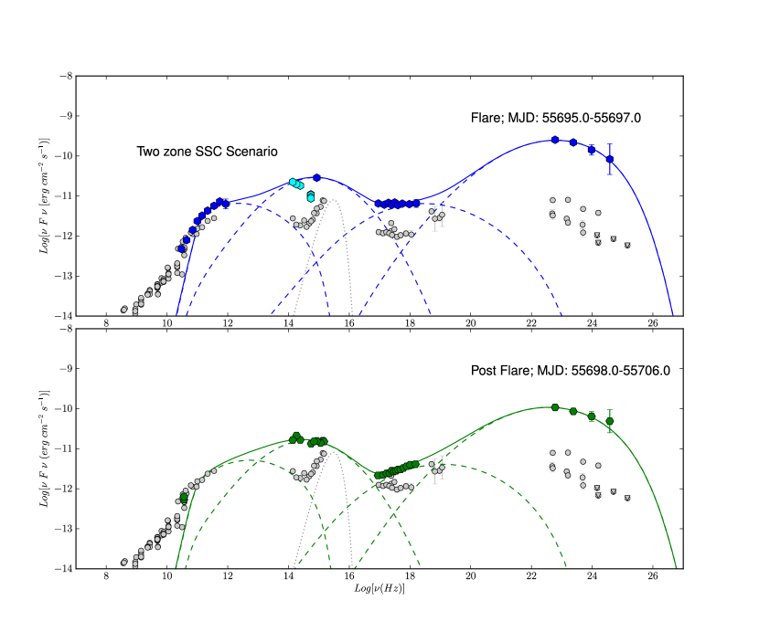
Figure 11: SED of 4C +49.22 at different epochs with fit models (solid lines) with a two-zone SSC code. The X- and $\gamma$-ray flare is evident. Simultaneous data during the flare of 2011 May 15 (MJD 55696) are shown in blue; the quasi-simultaneous data of CSS and INAOE are shown in cyan; post flare (i.e. Fermi-LAT and Swift-XRT data are integrated from 2011 May 17 to 25, MJD 55698-55706) data are shown in green; archival or low state data are shown in grey. The grey dashed lines represent the different components, synchrotron and inverse compton, used in the fitting procedure relative to each zone. The dotted line is the estimated contribution coming from the disc fitted to archival data.

A single flaring emission zone with a leptonic SSC process is a model often used for high-energy peaked (and TeV) blazars. This scenario represents the first step in SED modeling attempts. One-zone models usually have difficulty reproducing highly variable states and composite X-ray spectra often observed in the SEDs of FSRQs and low/intermediate energy peaked BL Lac objects. In this view a two-zone SSC model was applied to fit the SED of 4C +49.22, which allows us to take into account, in the fit attempt, the soft X-ray excess and the XRT spectral shape for the flare state of 2011 May 15 (characterised by a photon index of 2.03 $\pm$ 0.06, Table 4), and allows us to connect in the fit the simultaneous XRT and LAT data. Double leptonic emission zones have been recently invoked to fit simultaneous blazar SED data (for example, Georganopoulos & Kazanas, 2003; Liu & Shen, 2007; Abdo et al., 2011b; Tavecchio et al., 2011; Moraitis & Mastichiadis, 2011), albeit at the expense of more free parameters.

The flare and post-flare epochs in the SED of 4C +49.22, based on simultaneous data and on archival data representative of the quiet state, are shown in Figure 11 with the two-zone SSC models.

The hypothesis of two regions emitting through the SSC process is recently used in several cases of SED modeling. For example, a scenario based on a first SSC emission region encompassing the whole jet cross-section plus a second, compact and energetic SSC emission region defined by a high-bulk Lorentz factor blob responsible for the rapidly varying $\gamma$-ray emission is used in some SED models (Tavecchio et al., 2011; Ghisellini & Tavecchio, 2008).

The two emitting blobs for 4C +49.22 are thought to represent a compact and faster emission region filled with fresh and high-energy electrons, and a larger, slower and diluted region accounting for the radio-band emission from older and lower-energy cooling electrons, representing the surrounding plasma of the jet. The $\gamma$-ray emission blob is modeled with a bulk Doppler factor ${\mathcal{D}}_{1}=21.1$, size $R_{1}=7.5\times 10^{15}$ cm, intensity of the tangled magnetic field in the region of $B_{1}=0.25$ G. The instantaneous electron injection is self-consistently balanced with particle escape on a time scale of the order of $t_{\rm esc}=R/c$.

The radio-band and hard X-ray emitting blob is reproduced using a much larger emitting region characterised by parameter values ${\mathcal{D}}_{2}=15$, $R_{2}=5.5\times 10^{16}$ cm, and $B_{2}=0.10$ G. Relativistic Doppler beaming factors of the two zones are found to be consistent with the range of values found in the maps made from 2008 up to 2012 of the MOJAVE program (Lister et al., 2013). These two regions move relativistically along the jet, oriented at an angle at least $\theta<38^{\circ}$ with respect to the line of sight.

The kinetic partial differential equation of this model describes the evolution of the particle energy distribution after the injection of freshly accelerated electrons, with an instantaneous rate $Q(\gamma)$ equal to a power law turning into a log-parabola function in the high-energy tail (Landau et al., 1986; Massaro et al., 2006) whose functional form is:

$$Q(\gamma)=\left\{\begin{array}[]{rl}(\gamma/\gamma_{0})^{-s}&\mbox{ if $\gamma\leq\gamma_{0}$ }\\ (\gamma/\gamma_{0})^{-\left(s+r~{}\log(\gamma/\gamma_{0})\right)}&\mbox{ if $\gamma>\gamma_{0}$}\end{array}\right.$$ (6)

where $\gamma_{0}$ is the energy at the turnover frequency, $s$ is the spectral index at the reference energy $\gamma_{0}$ and $r$ is the spectral curvature. The respective values of parameters for both zones are reported in Table 11 for the flaring phase and Table 12 for the post-flare decreasing activity.

7.2 Single zone, SSC and ERC processes

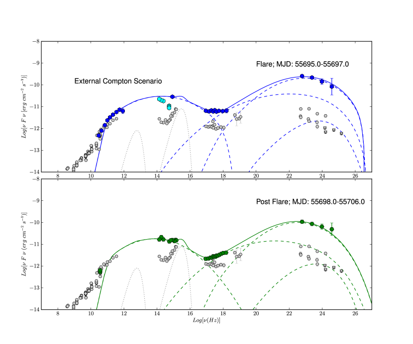
Figure 12: SED of 4C +49.22 at different epochs and relative fit models (solid lines) with a single zone and two-processes, SSC and ERC on disc and torus, code. Simultaneous data during the flare of May 15 are shown in blue; the quasi-simultaneous data of CSS and INAOE are shown in cyan; post flare (i.e. Fermi-LAT and Swift-XRT data are integrated from May 17 to 25) data are shown in green; archival or low state data are shown in grey. The grey dashed lines represent the different components, synchrotron and inverse compton, used in the fitting procedure. The dotted line is the estimated contribution coming from the disc fitted to archival data and the torus.

The high-power MeV-GeV bolometric emission seen in flaring $\gamma$-ray FSRQs, can usually be better described by external-jet Comptonisation of radiation (ERC) models. In this case the seed photons for the IC process are typically UV photons generated by the accretion disk surrounding the black hole, and reflected toward the jet by the Broad Line Region (BLR) clouds within a typical distance from the accretion disk of the order of 1 pc (Sikora et al., 1994). Another component of external-jet seed photons in the IR band for the scattering is likely provided by a dust torus (DT, see, e.g. Sikora et al., 2002). In this case the cooling of relativistic electrons is dominated by Comptonization of near and mid-IR radiation from ambient dust of the torus. This behaviour has already been found in FSRQs in the EGRET era (e.g., Sokolov & Marscher, 2005; Sikora et al., 2002, 2008, 2009). A model taking into account leptonic SSC emission with the relevant addition of leptonic ERC from a single active blob (the single zone two-process model) can also be used to explain the two-epoch SEDs of 4C +49.22 as shown in Figure 12. An accretion disc emission component is clearly seen in our archival data of the quiet activity state (bottom panel of Figure 12) and this could be the origin of the dominant inverse Compton $\gamma$-ray radiation. In the SSC plus ERC hybrid model for 4C +49.22 , X-ray emission can still be fitted as an SSC process, while the MeV-GeV $\gamma$-ray emission detected by Fermi can be fit well by dominant ERC emission from the thermal disc, DT and BLR dissipation region. For this model fit an equilibrium version of the time-dependent jet model reported in Tramacere et al. (2011) was used.

For the ERC emission, all the direct accretion disc radiation field, accretion disc emission reprocessed in the BLR and the radiation field from the DT illuminated by the disc are taken into account. We assumed the same electron energy distribution $Q(\gamma)$ with functional form equal to a power-law turning into a log-parabola function in the high-energy tail described above, for the single active zone emitting via SSC and ERC processes. In this case the single emitting blob is modeled with ${\mathcal{D}}=20.1$, $R=6.6\times 10^{16}$ cm and $B=0.10$ G. We estimated an accretion disc with physical characteristics using the UV data. We used the observations during the lowest phase of our dataset to constrain the clear sign of thermal emission coming from the accretion disc and set a reference value of $L_{disc}\simeq 4\times 10^{45}$ erg s^-1. The temperature profile of a standard disc emitting locally as a black-body following Ghisellini & Tavecchio (2009) is

$$T_{disc}^{4}(R)=\frac{3R_{S}L_{disc}}{16\pi\epsilon\sigma_{SB}R^{3}}\left(1-\sqrt{\frac{3R_{s}}{R}}\right)$$ (7)

where $\sigma_{SB}$ is the Stefan-Boltzmann constant and $R_{S}=2GM_{BH}/$c² is the Schwarzschild radius. We assumed that the accretion disc extends from $R_{in}\simeq 3R_{S}$ to $R_{out}\simeq 500R_{s}$. Since $T_{disc}(R)$ peaks at $R\simeq 4R_{S}$ we used the UV observations of the accretion disc to constrain the $T_{disc}$ and use Equation 7 to calculate $R_{S}$. Using our set of data, we extracted a value of $T_{disc}\simeq 5\times 10^{4}$ K. Assuming an accretion efficiency $\epsilon\simeq 0.1$, we obtain a $R_{s}\simeq 1.2\times 10^{14}~{}$cm. The value of BH mass $M_{BH}$ coming from the $R_{S}$ evaluation is about $4.0\times 10^{8}M_{\odot}$. This value of $M_{BH}$ we found using the UV observations of the accretion disc is compatible, assuming an accretion rate of 0.74 $M_{\odot}/$yr (coming from the formula that links the luminosity to the accretion mass rate $L_{disc}=\eta\dot{M}c^{2}$ erg/s) with the one obtained by Shields et al. (2003) using the virial assumption with the evaluation of FWHM of the broad H$\beta$ line. However it is less than the mass of the BH extracted by Decarli et al. (2008) using the estimation of the luminosity of the host galaxy. The BLR is represented as a spherical shell of reprocessing material with radial Thomson depth $\tau_{\rm BLR}=0.1$. If $L_{disc}=\eta\dot{M}c^{2}$ erg/s is the total luminosity of the disc (where $\eta$ is the accretion efficiency) the BLR is assumed to be a shell located at a distance from the central black hole of $r_{BLR}=10^{17}\sqrt{L_{disc}/10^{45}}$ cm (Ghisellini & Tavecchio, 2008). The energy dissipation, if it is assumed to be producing the $\gamma$-ray flux, must occur at hundreds of Schwarzschild radii from the black hole, in order to avoid $\gamma\gamma$ pair production absorption. Similarly the DT is placed at distance from the central black hole of $r_{\rm DT}=1\times 10^{19}$ cm. In our model we fixed values for the distance where the energy dissipation occurs within the BLR region, $r_{\rm BLR}^{min}=1\times 10^{18}$ cm and $r_{\rm BLR}^{max}=2\times 10^{18}$ cm during the first flare 2011 May 15 and the post flare phase of 2011 May 17-25. This implies an emission region placed at about 0.32 - 0.65 pc from the central black hole, in agreement with previous ERC scenarios for FSRQs (Dermer et al., 2009; Ghisellini & Tavecchio, 2009).

Both the two-zone SSC and single zone SSC+ERC models fits appear appropriate to represent the observed high-state and post-flare SED of 4C +49.22 built for the first time with simultaneous data from the three space missions Fermi, Swift and Planck. Equipartition ratio values, numbers of emission components, number of needed model fit parameters, their physical values, the agreements with previous models and VLBA data can alternatively support both scenarios. The manifest thermal blue-bump is completely overwhelmed by the non-thermal synchrotron emission during the flare, evidence which favours the double-zone SSC picture. Taking into account the multi-epoch VLBA results presented in Section 5.1 can exclude flaring GeV emission produced by jet knots placed at large distance, of the order of tens of parsecs (Lister et al., 2013), from the radio core and the BLR region. This can support a more canonical SSC+ERC model for FSRQ sources over the two-zone SSC, because active regions, if located at sub-parsec distances, would lie in proximity of the BLR photon field and if located within a few parsecs would lie at the scale of the molecular dust torus IR photon environment available for Comptonization.

Table 11: SED modeling parameters using a single zone SSC+ERC and a two zones SSC for the flare period (blue/filled points in Figures 11 and 12). ^∗ indicates that the parameters are frozen to typical values. ^∗∗ Value obtained describing the archival data.

Parameters	SSC(slow)+SSC(fast)	SSC+ERC
$\chi_{red}^{2}$	0.29	0.44
$\log_{10}(R)\textrm{[cm]}$	16.74∗/15.88$\pm$1.06	16.82$\pm$0.23
B [G]	0.10∗/0.25$\pm$0.04	0.10$\pm$0.13
$\mathcal{D}$	15∗/21.1$\pm$0.4	20.1$\pm$1.2
$N[\textrm{cm}^{-3}]$	2649.1$\pm$105.3/408.9$\pm$59.9	176.9$\pm$19.9
$\log_{10}(\gamma_{min})$	0.3∗/1.9$\pm$0.8	1.19$\pm$1.05
$\log_{10}(\gamma_{max})$	4∗/6∗	5.50$\pm$1.07
LogParab.+Power-law
$\log_{10}(\gamma_{0})$	1.78∗/2.77$\pm$1.26	1.83$\pm$0.43
r	0.8∗/1.11$\pm$0.54	0.43$\pm$0.05
s	1.23$\pm$0.04/0.54$\pm$0.12	1.32$\pm$0.72
Disc ∗∗ $-$ BLR $-$ DT
$L_{disc}$ [erg/s]	$-$	$4\times 10^{45}$
$T_{disc}^{max}$ [∘K]	$-$	$5\times 10^{4}$
$r_{BLR}^{min}$ [cm]	$-$	$1\times 10^{18}$
$r_{BLR}^{max}$ [cm]	$-$	$2\times 10^{18}$
$\tau_{BLR}$	$-$	0.1
$r_{DT}$ [cm]	$-$	$1\times 10^{19}$
$\tau_{DT}$	$-$	0.1

Table 12: SED modeling parameters using a single zone SSC+ERC and a two zones SSC for the post-flare period (green/filled points in Figures 11 and 12). ^∗ indicates that the parameters are frozen to a typical values. ^∗∗ Value obtained describing the archival data.

Parameters	SSC(slow)+SSC(fast)	SSC+ERC
$\chi_{red}^{2}$	0.23	0.20
$\log_{10}(R)\textrm{[cm]}$	16.74∗/15.92$\pm$0.76	16.63$\pm$0.77
B [G]	0.1∗/0.07$\pm$0.02	0.12$\pm$0.09
$\mathcal{D}$	15∗/33.3$\pm$1.9	22.9$\pm$5.4
$N[\textrm{cm}^{-3}]$	640.6$\pm$22.9/434$\pm$15.3	275.2$\pm$16.1
$\log_{10}(\gamma_{min})$	0.3∗/0.0009$\pm$0.0001	1.74
$\log_{10}(\gamma_{max})$	4.0∗/6.0∗	10.4$\pm$5.3
LogParab.+Power-law
$\log_{10}(\gamma_{0})$	1.77∗/2.77$\pm$0.51	1.66$\pm$0.31
r	0.8∗/1.04$\pm$0.27	0.52$\pm$0.17
s	0.9$\pm$0.1/0.7$\pm$0.2	1.06$\pm$0.15
Disc ∗∗ $-$ BLR $-$ DT
$L_{disc}$ [erg/s]	$-$	$4\times 10^{45}$
$T_{disc}^{max}$ [∘K]	$-$	$5\times 10^{4}$
$r_{BLR}^{min}$ [cm]	$-$	$1\times 10^{18}$
$r_{BLR}^{max}$ [cm]	$-$	$2\times 10^{18}$
$\tau_{BLR}$	$-$	0.1
$r_{DT}$ [cm]	$-$	$1\times 10^{19}$
$\tau_{DT}$	$-$	0.1

8 Discussion and conclusions

We have presented simultaneous Fermi, Swift and Planck, optical and near-IR flux observations and radio-band flux-structure observations of the blazar 4C +49.22 (S4 1150+49, OM 484, SBS 1150+497, $z=0.334$). This is one of few cases where time-simultaneous data from three such space missions are available, in particular during a bright GeV flare.

The GeV outburst of this FSRQ was observed by the LAT around 2011 May 15 after a prolonged period of low $\gamma$-ray activity. The $\gamma$-ray flare was observed simultaneously in X-ray data, with no measurable time lag (Figure 9). 4C +49.22 showed synchrotron emission peaked in the near-IR and optical wavebands with X-ray spectral softening and time-correlated variability in microwave/X-ray/GeV energy bands as observed more commonly in BL Lac objects rather than FSRQs. As seen in Section 7 the single SSC mechanism, adopted usually for BL Lac objects, can also explain the radio-to-gamma-ray SED of this FSRQ during the flaring state and following epoch (Figures 11 and 12).

This is also one of the first cases where a two-zone SSC model (slow+fast in-jet components) and a single-zone SSC+ERC model (BLR and DT components) both appear appropriate to represent the high $\gamma$-ray state multifrequency SED of a FSRQ. Opposite to the majority of the “strawman” models overimposed to SED data, our claim follows a true SED modeling through the best-fit model calculations with minimisation over the physical parameter grid (Tramacere et al., 2011).

We briefly recall the several aspects that make 4C +49.22 a particularly interesting object for high-energy studies. 4C +49.22 is a powerful and core-dominated FSRQ showing a bright and structured kiloparsec X-ray jet, diffuse thermal soft X-ray emission produced by the host galaxy and/or galaxy group medium, and a significant fluorescent $K\alpha$ emission line (equivalent width $\simeq 70$ eV) from cold Iron (Gambill et al., 2003; Sambruna et al., 2006b). The Fe line detection indicates that even in the X-ray band the beamed jet emission in the low activity states does not completely swamp the accretion-related emission, qualifying this source as a good candidate to investigate the disc-jet connection with multi-frequency observations (Grandi & Palumbo, 2004). This object is also a high luminosity FSRQ characterised by a one-sided core-jet radio structure, where the strong and compact jet extends 6 mas (i.e. about 28 pc) in the south-west direction. The 5 GHz VLBI polarisation structure of the source is relatively simple (Qi et al., 2009), where fractional polarisation ($\sim$1%) is basically concentrated in the core region, and the direction of the mas-scale magnetic field is consistent with jet direction. Chandra resolved and identified in a hot spot of 4C +49.22  and compact X-ray substructures (Tavecchio et al., 2005). Finally simultaneous disc and BLR luminosities show $L_{BLR}/L_{disc}=0.08$ (Sambruna et al., 2006b) and the estimated mass of the SMBH of 4C +49.22 is $4.0\times 10^{8}M_{\odot}$ consistent with what was found by Shields et al. (2003) and Decarli et al. (2008). Our results can be summarised as follows.

8.1 A class-transitional FSRQ ?

4C +49.22 is an FSRQs showing a shift of two orders of magnitude in the frequency of the synchrotron peak (from $\sim 10^{12}$ Hz to $\sim 10^{14}$ Hz) during the GeV $\gamma$-ray flare. This was accompanied by a contemporaneous marked spectral change in the X-ray energy band. In particular Giommi et al. (2012a) have shown that the distribution of synchrotron emission peaks of FSRQs are centred on a frequency of $10^{13}$ Hz, and the change seen in 4C +49.22 can be interpreted as phenomenological transition from a FSRQ to a BL Lac object, with the thermal blue-bump overwhelmed by synchrotron jet emission during the flaring state. This phenomenology can be taken into account in blazar classification and demography paradigms (Giommi et al., 2012b, 2013) even if occurring in short, transitory, phases of the blazar’s life, and can be in agreement with some recent hypotheses suggesting a smooth transition between the division of blazars into BL Lac objects and FSRQs (e.g., Cavaliere & D’Elia, 2002; Giommi et al., 2012b; Sbarrato et al., 2012). An example of a similar SED peak shift for flaring states is represented by the well-known FSRQ PKS 1510$-$089 (Abdo et al., 2010d; D’Ammando et al., 2011).

The marked spectral softening of the X-ray spectrum, providing an unusual flat X-ray SED, is also a feature observed in intermediate synchrotron energy peaked BL Lac objects rather than FSRQs. In addition this soft X-ray spectrum does not show any distinct sign of a bulk-Compton origin, generated by the adiabatic expansion of the emitting region and a cold population of electrons, a feature found usually in FSRQs but missing in this case. SED data therefore suggest a contribution to the X-ray emission from different emission components, i.e. both synchrotron and inverse Compton (SSC and/or ERC) mechanisms, as usually observed for intermediate energy peaked BL Lac objects (for example Tagliaferri et al., 2000; Ciprini et al., 2004; Abdo et al., 2011c).

Another interesting feature related to this is the optical spectrum. SSDS DR7 and DR8 optical spectra (Adelman-McCarthy et al., 2008), obtained during low emission states, show a rest frame equivalent width (EW) of the broad $H{\alpha}$ emission line of about 300 Å. We fitted the synchrotron bump of the SED during the $\gamma$-ray flare epoch using a third degree polynomial function and we extrapolated using the best-fit model the value of the continuum at the $H{\alpha}$ frequency. Provided that flux enhancement is due to non-thermal radiation only, the extrapolated continuum of 4C +49.22 at the frequency of the $H{\alpha}$ emission line shows an increase of a factor of $\sim 23$ during the $\gamma$-ray flaring state, resulting in a reduction of the emission line EW to about 13Å, therefore approaching the limit considered for the BL Lac object class (blazars with rest-frame emission line equivalent widths smaller than 5Å). The usual classification of blazar subclasses using the rest frame EW definition can be misleading. Objects so far classified as BL Lac objects are turning out to be two physically different classes: intrinsically weak lined objects, more common in X-ray selected samples, and heavily jet-diluted broad lined sources, more frequent in radio selected samples (Giommi et al., 2012b, 2013).

8.2 Two-zone SSC vs single zone SSC+ERC models

The multi-frequency SEDs (Figures 11 and 12) show the synchrotron emission outshining the thermal blue-bump emission that appeared evident in the low activity state. We modeled the radio-to-gamma-ray SEDs for the flare state and the post-flare epoch. A single flaring blob with two different emission mechanisms (SSC and ERC) and a two-zone model with a single SSC process were applied to our SED data. The averaged low state built with archival data (gray points and blue bump signature in Figures 11 and 12) can be described by including both the jet and disc contributions while the single zone SSC model fails. The disc emission is parametrized in terms of a blackbody from optical to soft X-rays, and the ERC modeling required also a torus emission component contributing to the IC scattering. Our two-zone SSC and single zone SSC+ERC model fits appears both appropriate to represent the observed high-state and post-flare SED of 4C +49.22, depending on the considered feature (equipartition ratio values, number of parameters, their values, agreements of parameters with previous model values estimated in literature, and agreement with VLBA parameter values and structure). The SSC+ERC is suggested to be slightly more preferred based on equipartition ratio, but the two-zone pure-SSC is still a valid alternative. The manifest thermal blue-bump is completely outshone by the non-thermal synchrotron emission during the flare, evidence which goes in the direction of the pure SSC scenario, that usually better represents the SEDs of BL Lac objects.

On the other hand, the multi-epoch VLBA results presented in Section 5.1 can exclude flaring GeV emission produced by jet knots placed at large distances, of the order of tens of parsecs (Lister et al., 2013), from the radio core and the BLR region. This suggests a non-negligible contribution of seed photons produced in the BLR for the IC up-scatter, strengthening the case for the hybrid SSC+ERC scenario. In general equipartition can be strongly violated during large $\gamma$-ray flare events. Previous SSC models applied to the SED of 4C +49.22 and fits of radio-to-X-ray emission of Chandra-resolved subcomponents seen in the terminal part of the jet (Tavecchio et al., 2005) support this violation. This suggests IC scattering of synchrotron radiation by some special electron distribution with an excess of high-energy electrons, or CMB photons, or back-scattered central radiation. Fermi-LAT detected non-spatially resolved GeV emission from 4C +49.22 and which may have been an integrated combination of emission from different regions. In this view the $\gamma$-ray flaring state (blue points in Figures 11 and 12) likely can be better represented by the double zone SSC scenario.

8.3 Pair production opacity and relativistic beaming

The $\gamma$-ray flux of 4C +49.22 is variable with short time scales ($<$ 1 day). The rapid variability and the large $\gamma$-ray luminosity imply appreciable pair production opacity. The unbeamed source size estimated from the observed variability timescale indicates that the source is opaque to the photon-photon pair production process if $\gamma$-ray and X-ray photons are produced cospatially. This assumption, however, firmly rests on the simultaneity of the flaring event as observed by Fermi-LAT and Swift-XRT. Simultaneous X-ray and $\gamma$-ray flare events have been measured in the past for other sources like 3C 454.3 (Abdo et al., 2009c). Relativistic beamed jet and emission blobs can solve this problem. Following the arguments given in Mattox et al. (1993) and adopting the doubling flux timescale of $t_{d}\sim 0.6$ days and the observed X-ray flux of $S_{X}=(2.1\pm 0.1)\times 10^{-11}~{}\mathrm{erg}~{}\mathrm{cm}^{-2}~{}\mathrm{s}^{-1}$ (as measured during the main flare in $\gamma$ rays) at the observed photon frequency $\nu_{X}\simeq 10^{18}$ Hz (corresponding to the photons that interact with the GeV $\gamma$ rays in the jet rest frame), we can estimate the Doppler factor $\mathcal{D}$ required for the photon-photon annihilation optical depth to be $\tau_{\gamma\gamma}<1$. With the derived relation:

$$\tau_{\gamma\gamma}\simeq\frac{\sigma_{T}d_{L}^{2}S_{X}}{3t_{d}c^{2}E_{X}\mathcal{D}^{4}}$$ (8)

where we assume the emission region linear size $R=ct_{d}\mathcal{D}/(1+z)\simeq 2\times 10^{16}$ cm and the source-frame photon energy $E_{X}=(1+z)h\nu_{x}/\mathcal{D}$. Assuming the standard cosmology values we obtain $\mathcal{D}\gtrsim 8.3$. Omitting the requirement of cospatiality of the X-ray and $\gamma$-ray emission regions relaxes this limit. This can be compared with the estimate obtained from the VLBA superluminal motion, $\mathcal{D}>4.3$. As long as the velocity of the VLBA jet is the same as the velocity of the outflow within the blazar emission zone, this implies that the photon-photon annihilation effects involving the X-ray emission generated within the jet are negligible.

8.4 Energy dissipation region

The location of the $\gamma$-ray emitting region is debated, although large distances from the black hole are recently being favored for about 2/3 of GeV FSRQs (e.g., Marscher et al., 2010). Ten epochs of VLBA observations at 15 GHz (MOJAVE program) of 4C +49.22 obtained from 2008 May to 2013 February point to Lorentz factor limits that are consistent with our SED modeling and to increasing flux density and polarisation degree in the radio core after the GeV $\gamma$-ray flare. In addition, Planck simultaneous observations reveal spectral changes in the sub-mm regime associated with the $\gamma$-ray flare. Our SED modeling is in agreement with multi-epoch VLBA results and takes into account this evolution observed between the flare on May 15 (blue SED data and Table 11) and the post-flare (May 17-25) epoch (green SED data and Table 12). The resulting compact emission region of 4C +49.22 suggests that nuclear optical/UV seed target photons of the BLR dominate the production of IC emission (Tavecchio et al., 2010). Alternatively if the volume involved in the $\gamma$-ray emission is assumed much smaller than jet length scales, like turbulent plasma cells flowing across standing shocks (Marscher, 2014), hour/day-scale variability can also be produced at several parsecs from the central engine. The VLBA flux density and polarisation degree in the radio core both increased with the ejection of a new component close in time to the $\gamma$-ray flare epoch. The jet kinetic power and disc luminosity of 4C +49.22 follow the same trend observed for other powerful $\gamma$-ray FSRQs, where a large fraction of the accretion power is converted into bulk kinetic energy of the jet, and our SED models suggest a larger BLR size compared to previous estimates (Decarli et al., 2008; Sambruna et al., 2006b).

    

The detailed results about 4C +49.22 presented in this work followed the availability of simultaneous Fermi, Swift, Planck and VLBA observations triggered by the LAT-detected GeV outburst and by our Swift ToO follow-up program. Such data allowed us to investigate multi-frequency flux versus radio-structure relationships, build and constrain pure-SSC vs SSC+ERC SED physical model fits, study emission region localisation, energetics and the evolution of the multi-frequency and high-energy SED during two different emission states for the source, and finally to extrapolate phenomenological features alternatively supporting the FSRQ or BL Lac nature of the source. 4C +49.22 is a powerful FSRQ, with a FR II morphology and possesses a powerful radio/X-ray jet, but it can have its broad emission lines heavily diluted by a swamping non-thermal continuum during high-energy events. The synchrotron peak energy and the unresolved X-ray spectra resemble those of intermediate BL Lac objects. Simultaneous multi-frequency data at low and high energies, from space-borne missions like Fermi, Swift, and Planck are also needed in the future to correctly draw conclusions about the underlying physics, demography and cosmological evolution of $\gamma$-ray loud AGN.

References

- Abdo et al. (2011b) Abdo, A. A., Ackermann, M., Ajello, M., et al. 2011b, ApJ, 730, 101
- Abdo et al. (2011c) Abdo, A. A., et al. 2011, ApJ, 730, 101
- Abdo et al. (2010a) Abdo, A. A., et al. 2010, ApJ, 722, 520
- Abdo et al. (2010b) Abdo, A. A., et al. 2010a, ApJs, 188, 405
- Abdo et al. (2010c) Abdo, A. A., et al. 2010b, ApJ, 716, 30
- Abdo et al. (2010d) Abdo, A. A., Ackermann, et al. 2010d, ApJ, 721, 1425
- Abdo et al. (2009a) Abdo, A. A., et al., 2009a, ApJs, 183, 46
- Abdo et al. (2009b) Abdo, A. A., et al., 2009b, Atropart. Physics, 32, 193
- Abdo et al. (2009c) Abdo, A. A., et al. 2009, ApJ, 699, 817
- Ackermann et al. (2012) Ackermann, M., et al. 2012, ApJs, 203, 4
- Ackermann et al. (2011a) Ackermann, M., et al. 2011, ApJ, 741, 30
- Ackermann et al. (2011b) Ackermann, et al. 2011, ApJ, 743, 171
- Ade et al. (2013) Ade, P. A. R., Aghanim, N., Armitage-Caplan, C. et al. 2013, submitted (arXiv:1303.5076)
- Adelman-McCarthy et al. (2008) Adelman-McCarthy, J. K., et al. 2008, ApJs, 175, 297
- Akujor & Garrington (1991) Akujor, C. E., & Garrington, S. T. 1991, MNRAS, 250, 644
- Atwood et al. (2009) Atwood, W. B., et al., 2009, ApJ, 697, 1071
- Barthelmy et al. (2005) Barthelmy, S. D., et al. 2005, Space Sci. Rev., 120, 143
- Böttcher et al. (2009) Böttcher, M., Reimer, A., & Marscher, A. P. 2009, ApJ, 703, 1168
- Burbidge (1968) Burbidge, E. M. 1968, ApJl, 154, L109
- Burrows et al. (2005) Burrows, D. N., et al. 2005, Space Sci. Rev., 120, 165
- Cavaliere & D’Elia (2002) Cavaliere, A., & D’Elia, V. 2002, ApJ, 571, 226
- Ciprini et al. (2004) Ciprini, S., Tosti, G.,Teräsranta, H., & Aller, H. D. 2004, MNRAS, 348, 1379
- Cohen et al. (2007) Cohen, A. S., Lane, W. M., Cotton, W. D., et al. 2007, AJ, 134, 1245
- Condon et al. (1998) Condon, J. J., Cotton, W. D., Greisen, E. W., et al. 1998, AJ, 115, 1693
- Cusumano et al. (2010a) Cusumano, G., et al. 2010, A&A, 524, A64
- Cusumano et al. (2010b) Cusumano, G., et al. 2010, A&A, 510, A48
- D’Ammando et al. (2011) D’Ammando, F., et al. 2011, A&A, 529, A145
- Decarli et al. (2008) Decarli, R., Labita, M., Treves, A., & Falomo, R. 2008, MNRAS, 387, 1237
- Dermer & Atoyan (2004) Dermer, C. D., & Atoyan, A. 2004, ApJL, 611, L9
- Dermer et al. (2009) Dermer, C. D., Finke, J. D., Krug, H., Böttcher, M. 2009, ApJ, 692, 32
- Dermer et al. (2014) Dermer, C. D., Cerruti, M., Lott, B., Boisson, C., & Zech, A. 2014, ApJ, 782, 82
- Dixon (1970) Dixon, R. S. 1970, ApJs, 20, 1
- Drake, et al. (2009) Drake, A.J. et al. 2009, ApJ, 696, 870
- Fanti et al. (2001) Fanti, C., Pozzi, F., Dallacasa, D., Fanti, R., Gregorini, L., Stanghellini, C. and Vigotti, M. 2001, A&A, 369, 380
- Finke et al. (2008) Finke, J. D., Dermer, C. D., Böttcher, M. 2008, ApJ, 686, 181
- Fitzpatrick (1999) Fitzpatrick, N. 1999, PASP, 111, 63
- Gambill et al. (2003) Gambill, J. K., et al. 2003, A&A, 401, 505
- Gehrels et al. (2004) Gehrels, N., et al. 2004, ApJ, 611, 1005
- Georganopoulos & Kazanas (2003) Georganopoulos, M., & Kazanas, D. 2003, ApJL, 594, L27
- Giommi et al. (2012a) Giommi, P., et al. 2012, A&A, 541, A160
- Giommi et al. (2012b) Giommi, P., et al. 2012, MNRAS, 420, 2899
- Giommi et al. (2013) Giommi, P., Padovani, P., Polenta, G. 2013, MNRAS, 431,1914
- Ghisellini et al. (2009) Ghisellini, G., Tavecchio, F., & Ghirlanda, G. 2009, MNRAS, 399, 2041
- Ghisellini & Tavecchio (2009) Ghisellini, G., & Tavecchio, F. 2009, MNRAS, 397, 985
- Ghisellini & Tavecchio (2008) Ghisellini, G., & Tavecchio, F. 2008, MNRAS, 386, L28
- González-Nuevo et al. (2006) González-Nuevo J., Argüeso F., López-Caniego M., Toffolatti L., Sanz J. L., Vielva P., Herranz D., 2006, MNRAS, 369, 1603
- Grandi & Palumbo (2004) Grandi, P., & Palumbo, G. G. C. 2004, Science, 306, 998
- Gregory et al. (1997) Gregory, P. C., Scott, W. K., Douglas, K., & Condon, J. J. 1996, ApJs, 103, 427
- Hartman et al. (1999) Hartman, R. C., Bertsch, D. L., Bloom, S. D., et al. 1999, ApJs, 123, 79
- Hardcastle (2006) Hardcastle, M. J. 2006, MNRAS, 366, 1465
- Hays & Donato (2011) Hays, E., & Dona, D. 2011, The Astronomer’s Telegram, 3313, 1
- Hunt et al. (1998) Hunt, L. K., et al. 1998, AJ, 115, 2594
- Kalberla et al. (2005) Kalberla, P. M. W., et al. 2005, A&A, 440, 775
- Kuehr et al. (1981) Kuehr, H., Witzel, A., Pauliny-Toth, I. I. K., & Nauber, U. 1981, A&AS, 45, 367
- Landau et al. (1986) Landau, R., et al. 1986, ApJ, 308, 78
- Leahy et al. (2010) Leahy, J. P., et al. 2010, A&A, 520, A8
- Linfield et al. (1983) Linfield, R. 1983, ApJ, 275, 461
- Lister et al. (2009) Lister, M. L., et al. 2009, AJ, 137, 3718
- Lister et al. (2013) Lister, M. L., Aller, M. F., Aller, H. D., et al. 2013, AJ, 146, 120
- Liu & Shen (2007) Liu, W.-P., & Shen, Z.-Q. 2007, ApJL, 668, L23
- León-Tavares et al. (2012) León-Tavares et al. 2012 ApJ, 754, 23
- León-Tavares et al. (2011) León-Tavares, J., Valtaoja, E., Tornikoski, M., Lähteenmäki, A., & Nieppola, E. 2011, A&A, 532, A146
- López-Caniego et al. (2006) López-Caniego, M., et al. 2006, MNRAS, 370, 2047
- López-Caniego et al. (2007) López-Caniego, M., et al. 2007, ApJs, 170, 108
- Lynds & Wills (1968) Lynds, R., & Wills, D. 1968, ApJl, 153, L23
- Moore & Stockman (1981) Moore, R. L., & Stockman, H. S. 1981, ApJ, 243, 60
- Mandolesi et al. (2010) Mandolesi, N., et al. 2010, A&A, 520, A3
- Marscher (2014) Marscher, A. P. 2014, ApJ, 780, 87
- Marscher (2006) Marscher, A. P. 2006, AIP Conf. Proc. 856, p.1
- Marscher et al. (2010) Marscher, A. P., et al. 2010, ApJ Lett, 710, L126
- Massardi et al. (2009) Massardi, M., et al. 2009, MNRAS, 392, 733
- Massaro et al. (2006) Massaro, E., Tramacere, A., Perri, M., Giommi, P., & Tosti, G. 2006, A&A, 448, 861
- Mattox et al. (1993) Mattox, J. R., et al. 1993, ApJ, 410, 609
- Mattox et al. (1996) Mattox, J. R., et al. 1996, ApJ, 461, 396
- Moraitis & Mastichiadis (2011) Moraitis, K., & Mastichiadis, A. 2011, A&A, 525, A40
- Nolan et al. (2012) Nolan, P. L., et al. 2012, ApJs, 199, 31
- Orienti et al. (2011) Orienti, M., Venturi, T., Dallacasa, D., D’Ammando, F., Giroletti, G., Giovannini, G., Vercellone, S., Tavani, M. 2011, MNRAS, 417, 359
- Owen & Puschell (1984) Owen, F. N., & Puschell, J. J. 1984, AJ, 89, 932
- Rosset et al. (2010) Rosset, C., et al. 2010, A&A, 520, A13
- Pei (1992) Pei, Y. C. 1992, ApJ, 395, 130
- Peterson et al. (1998) Peterson, B. M. et al., 1998, PASP, 110, 660
- Pittori et al. (2009) Pittori, C., Verrecchia, F., Chen, A. W., et al. 2009, A&A, 506, 1563
- Planck HFI Core Team et al. (2011) Planck HFI Core Team, 2011, A&A, 536, A4
- Planck Collaboration et al. (2011) Planck Collaboration, 2011, A&A, 536, A2
- Planck HFI Core Team et al. (2011) Planck HFI Core Team, 2014, A&A in press; arXiv:1101.2039
- Planck Collaboration et al. (2011) Planck Collaboration, 2011, A&A, 536, A1
- Planck HFI Core Team et al. (2011) Planck HFI Core Team, 2011, A&A, 536, A6
- Planck Collaboration et al. (2011) Planck Collaboration, 2011, A&A, 536, A7
- Planck Collaboration et al. (2013) Planck Collaboration XXVIII, 2014, A&A in press; arXiv:1303.5088
- Planck Collaboration et al. (2013) Planck Collaboration II, 2014, A&A in press; arXiv:1303.5063
- Planck Collaboration et al. (2013) Planck Collaboration I, 2014, A&A in press; arXiv:1303.5062
- Planck Collaboration et al. (2013) Planck Collaboration VI, 2014, A&A in press; arXiv:1303.5067
- Poole et al. (2008) Poole, T.S., et al. 2008 MNRAS, 383, 627
- Pushkarev et al. (2009) Pushkarev, A. B., Kovalev, Y. Y., Lister, M. L., & Savolainen, T. 2009, A&A, 507, L33
- Qi et al. (2009) Qi, J.-W., Zhang, H.-Y., & Nan, R.-D. 2009, Chinese A&A, 33, 251
- Reyes et al. (2011) Reyes, L., D’Ammando, F., & Hoversten, E. 2011, ATel, 3353, 1
- Roming et al. (2005) Roming, P. W. A., Kennedy, T. E., Mason, K. O., et al. 2005, SSRv, 120, 143
- Roming et al. (2005) Roming, P. W. A., Kennedy, T. E., Mason, K. O., et al. 2005, Space Sci. Rev., 120, 95
- Sambruna et al. (2006a) Sambruna, R. M., Gliozzi, M., Donato, D., Maraschi, L., Tavecchio, F., Cheung, C. C., Urry, C. M., Wardle, J. F. C. 2006, ApJ, 641, 717
- Sambruna et al. (2006b) Sambruna, R. M.,Gliozzi, M., Tavecchio, F., Maraschi, L., & Foschini, L. 2006, ApJ, 652, 146
- Sambruna et al. (2004) Sambruna, R. M., et al. 2004, ApJ, 608, 698
- Savolainen et al. (2010) Savolainen, T., et al. 2010, A&A, 512, A24
- Sbarrato et al. (2012) Sbarrato, T., Ghisellini, G., Maraschi, L., & Colpi, M. 2012, MNRAS, 421, 1764
- Sikora et al. (2002) Sikora, M., Begelman, M. C., & Rees, M. J. 1994, ApJ, 421, 153
- Sikora et al. (2009) Sikora, M., Stawarz, Ł., Moderski, R., Nalewajko, K., & Madejski, G. M. 2009, ApJ, 704, 38
- Sikora et al. (2008) Sikora, M., Moderski, R., & Madejski, G. M. 2008, ApJ, 675, 71
- Sikora et al. (1994) Sikora, M., Begelman, M. C., & Rees, M. J. 1994, ApJ, 421, 153
- Schlegel et al. (1998) Schlegel, D. J., Finkbeiner, D. P., & Davis, M. 1998, ApJs, 500, 525
- Shields et al. (2003) Shields, G. A., Gebhardt, K., Salviander, S., et al. 2003, ApJ, 583, 124
- Stepanian et al. (2001) Stepanian, J. A., Green, R. F., Foltz, C. B., et al. 2001, AJ, 122, 3361
- Schlegel et al. (1998) Schlegel, D.J., Finkbeiner D.P., and Davis, M., 1998, ApJ, 500, 525
- Sokolov & Marscher (2005) Sokolov, A., & Marscher, A. P. 2005, ApJ, 629, 52
- Tagliaferri et al. (2000) Tagliaferri, G., et al. 2000, A&A, 354, 431
- Tauber et al. (2010) Tauber, J. A., et al. 2010, A&A, 520, A1
- Tavecchio et al. (2010) Tavecchio, F., Ghisellini, G., Bonnoli, G., & Ghirlanda, G. 2010, MNRAS, 405, L94
- Tavecchio et al. (2011) Tavecchio, F., Becerra-Gonzalez, J., Ghisellini, G., et al. 2011, A&A, 534, A86
- Tavecchio et al. (2005) Tavecchio, F., Cerutti, R., Maraschi, L., Sambruna, R. M., Gambill, J. K., Cheung, C. C., Urry, C. Megan 2005, ApJ, 630, 721
- Teräsranta et al. (1998) Teräsranta, H., Tornikoski, M., Mujunen, A. et al. 1998, A&AS, 132, 305
- Tramacere et al. (2009) Tramacere, A., Giommi, P., Perri, M., Verrecchia, F., & Tosti, G. 2009, A&A, 501, 879
- Tramacere et al. (2011) Tramacere, A., Massaro, E., & Taylor, A. M. 2011, ApJ, 739, 66
- White et al. (1994) White, N. E., Giommi, P., & Angelini, L. 1994, IAU Circ, 6100, 1
- White et al. (1997) White, R. L., Becker, R. H., Helfand, D. J., & Gregg, M. D. 1997, ApJ, 475, 479
- Wright et al. (2009) Wright, E. L., Chen, X., Odegard, N., et al. 2009, ApJs, 180, 283
- Voges et al. (1999) Voges, W., Aschenbach, B., Boller, T., et al. 1999, A&A, 349, 389
- Zacchei et al. (2011) Zacchei, A., et al. 2011, A&A, 536, A5