Abstract

The all-sky maps of the observed variation of the Hubble constant can be reproduced from a theoretical point of view by introducing an intergalactic plasma with a variable number density of electrons. The observed averaged value and variance of the Hubble constant are reproduced by adopting a rim model, an auto-gravitating model, and a Voronoi diagrams model as the backbone for an auto-gravitating medium. We also analyze an astronomer’s model based on the 3D spatial distribution of galaxies as given by the 2MASS Redshift Survey and an auto-gravitating Lane–Emden ($n=5$) profile of the electrons. The simulation which involves the Voronoi diagrams is done in a cubic box with sides of 100 Mpc. The simulation which involves the 2MASS covers the range of redshift smaller than 0.05.

Adv. Studies Theor. Phys, Vol. x, 200x, no. xx, xxx - xxx

Anisotropy in the Hubble constant as modeled by density gradients

L. Zaninetti

Dipartimento di Fisica,

Università degli Studi di Torino,

via P. Giuria 1, 10125 Torino, Italy

Keywords: Galaxies; Clusters of galaxies; Distances, redshifts, radial velocities; Observational cosmology

1 Introduction

Hubble’s constant [1] is characterized at the moment of writing by a large uncertainty. A recent evaluation, see [2], quotes

$$H_{0}=(74.3\pm 2.1)\mathrm{km\,s^{-1}\,Mpc^{-1}}\quad,$$ (1)

which means a relative standard uncertainty of 28264 parts per million (in the following ppm). As a comparison, the value of the Newtonian gravitational constant, denoted by $G$, is

$$G=(6.67384\,10^{-11}\pm 0.0008)m^{3}kg^{-1}s^{-2}\quad,$$ (2)

which means an uncertainty of 120 ppm, see [3]. Hubble’s constant is actually much used in the series of models starting with [4, 5] as well as in the modern theories on the accelerating universe, see [6, 7]. In this standard cosmology the Hubble parameter is defined as

$$H=\frac{\dot{a}}{a}\quad,$$ (3)

where a(t) is the scale factor. The currently observable value of the Hubble constant is H₀ and in the standard cosmology is independent of the chosen line of sight of the observer situated on the Earth. A different explanation for Hubble’s constant lies in the momentum lost by the light during the travel in the intergalactic medium (IGM). The first formula for the change of frequency of the light in a gravitational framework was due to [8]:

$$\frac{\Delta\nu}{\nu}=\frac{1.4\pi G\rho DL}{c^{2}}\quad.$$ (4)

Here, $\nu$ is the considered frequency, $G$ is the Newtonian gravitational constant, $\rho$ is the density in g/cm³, $D$ is the distance after which the perturbing effect begins to fade out, $L$ is the considered distance, and $c$ is the speed of light. The study of the physical mechanisms which produce the redshift of light was dormant for 70 years but currently is explained by different physical models. We list some of the processes which produce the observed redshift of galaxies:

• a plasma physics effect, see [9, 10],

• a photo-absorption process, see [11],

• an interaction of photons with curved space time, see [12, 13],

• an interaction of photons with intergalactic free electrons, see [14],

• an interaction between single photons traveling across the micro-quanta flux, see [15].

The detailed analysis of these and other physical mechanisms which produce the observed redshift can be found in [16].

The explanation of the anisotropies in Hubble’s constant started with [17] analyzing the Markarian galaxies. The deviations from the Hubble flow for the brightest galaxies were analyzed in [18]. A self similar cosmology was applied to explain the anisotropies in Hubble’s constant, see [19]. The radial and angular variance in the Hubble flow are derived on scales in which the flow is in the nonlinear regime, see [20]. In this paper, Section 4 reviews the existing data on the anisotropy of the Hubble constant and two plasma effects within the IGM which produce the observed redshift. Section 2 reports the standard approach to the accelerating universe. Section 3 reviews the current status of the astronomical observations which point towards a non-homogeneous local universe. Section 5 introduces two simple models based on the average value of the cosmic voids which produce an anisotropy in the Hubble constant. Section 6 introduces a Voronoi diagrams network for the 3D spatial distribution of galaxies and a logistic distribution for the number density of electrons, which leads to an anisotropy in the Hubble constant. Section 7 inserts the 3D spatial distribution of galaxies as given by a recent catalog a number density profile of electrons of the Emden type: as a consequence, contour maps of the Hubble constant are generated.

2 Standard Cosmology

The field equations in general relativity (GR), after [21], are

$$R_{\mu\nu}-\frac{g_{\mu\nu}R}{2}=-\kappa\,T_{\mu\nu}$$ (5)

with

$$\kappa=\frac{8\pi G}{c^{4}}\quad,$$ (6)

where $R_{\mu\nu}$ is the Ricci tensor of the first kind, $g_{\mu\nu}$ is the metric tensor, $T_{\mu\nu}$ is the energy–momentum tensor, R is the Ricci scalar, G is the gravitational constant, and c is the speed of light. The introduction of the cosmological constant $\Lambda$, see [22, 23], transforms the previous equations into

$$R_{\mu\nu}-\frac{g_{\mu\nu}R}{2}-\Lambda g_{\mu\nu}=-\kappa\,T_{\mu\nu}\quad.$$ (7)

On inserting the Friedmann–Robertson–Walker (FRW) metric and the perfect fluid tensor into the Einstein equations, we obtain the Friedmann equation

$$\left({\dot{a}(t)\over a(t)}\right)^{2}={8\pi G\over 3}\,\rho+{\Lambda c^{2}\over 3}-{\kappa c^{2}\over a(t)^{2}}\quad,$$ (8)

where $\rho$ is the density, $\kappa$ takes the values -1,0,1 for negative, zero, or positive spatial curvature, and $a(t)$ is the scale factor, see [4, 5]. The previous equation has been deduced calculating the volume, $V$, of the 3D hypersphere

$$V=2\,\pi^{2}\,a(t)^{3}$$ (9)

and the total mass, M,

$$M=\rho\,V\quad.$$ (10)

This means that the local universe is assumed to be homogeneous, $\rho$ is constant, and isotropic, the integration for the volume over the three angles is standard. The study of 42 supernovae of type Ia in [7] suggested an expanding universe with acceleration. The acceleration can be explained by introducing the dark matter parameter $\Omega_{\Lambda}$, where the index $\Lambda$ indicates its similarity with the cosmological constant. The Friedmann equation now is

$$\frac{\dot{a}^{2}}{a^{2}}+\frac{H_{0}^{2}(\Omega_{0}-1)}{a^{2}}=H_{0}^{2}(\frac{\Omega_{m}}{a^{3}}+\frac{\Omega_{r}}{a^{4}}+\Omega_{\Lambda})\quad,$$ (11)

where the actual energy density parameter, $\Omega_{0}$, is given by the sum of matter, radiation, and dark components

$$\Omega_{0}=\Omega_{m}+\Omega_{r}+\Omega_{\Lambda}$$ (12)

and $H_{0}$ is the current value of the Hubble constant, see [24] for more details. A recent evaluation gives a dark energy density $\Omega_{\Lambda}$ =0.7185, a matter density $\Omega_{m}$ =0.235, $H_{0}=69.7,\mathrm{km\,s^{-1}\,Mpc^{-1}}$, and age of the universe $t_{0}$ = 13.76 Gyr. With these parameters, Figure 1 shows the temporal behavior of the scale factor as given by the solution of (11).

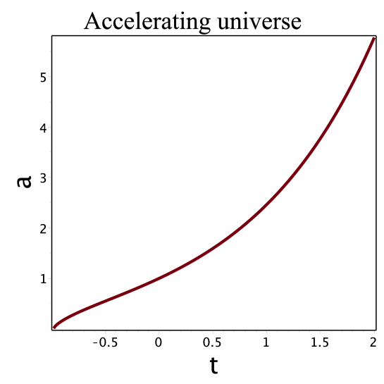
Figure 1: Evolution of the scale factor from the singularity at $t=-1$, to $t=2$.

3 The non-homogeneous universe

The standard cosmology is based on the concept of a homogeneous and isotropic universe. Recent observations point instead towards a cellular structure of the local universe. As an example, we report the 2dF Galaxy Redshift Survey (2dFGRS) catalog when a slice of $75^{\circ}\times 3^{\circ}$ is considered, see Figure 2.

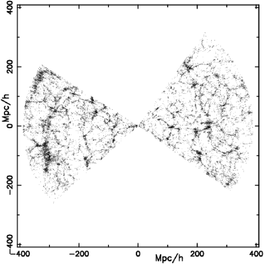
Figure 2: Slice of $75^{\circ}\times 3^{\circ}$ in the 2dFGRS. This plot contains 30000 galaxies and belongs to the 2dFGRS available at http://msowww.anu.edu.au/2dFGRS/  .

The observational fact that the spatial position is digitized allows us to map the Newtonian gravitational field. We firstly express the Newtonian gravitational constant in the following astrophysical units: length in Mpc, mass in M${}_{\mbox{gal}}$ which is $10^{11}M_{\hbox{$\odot$}}$ and yr₈ which are $10^{8}$ yr:

$$G=4.49975\,10^{-6}\frac{\mbox{Mpc}^{3}}{M_{\mbox{gal}}\mbox{yr}_{8}^{2}}\quad.$$ (13)

To each galaxy we associate a mass of $10^{12}M_{\hbox{$\odot$}}=10M_{\mbox{gal}}$ and we evaluate the gravitational force, expressed in $\frac{\mbox{Mpc}M_{\mbox{gal}}}{\mbox{yr}_{8}^{2}}$, on a unitarian mass, 1$M_{\mbox{gal}}$. For practical purposes in each point of a 2D grid made by 500$\times$500 points we compute the gravitational force, $\overrightarrow{F}$ by

$$\overrightarrow{F}=-\sum_{i=1}^{N}G\frac{M_{i}}{r_{i}^{3}}\overrightarrow{r}\quad,$$ (14)

where the index $i$ runs from 1 to the number of considered galaxies, $N$, $M_{i}$ is the mass of the considered galaxy, $10M_{\mbox{gal}}$, $\overrightarrow{r}$ is the distance between the grid’s point and the considered galaxy, and $G$ is the Newtonian constant of gravitation expressed in $\frac{\mbox{Mpc}^{3}}{M_{\mbox{gal}}\mbox{yr}_{8}^{2}}$. Figure 3 reports a 2D map of the modulus of such force and Figure 4, a cut in the middle of such a map.

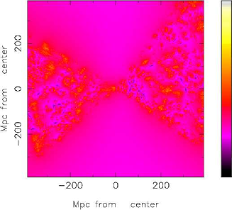
Figure 3: Map of the decimal logarithm of the modulus of the gravitational force for 2dFGRS.

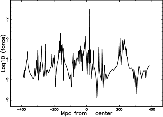
Figure 4: Cut along the center for the decimal logarithm of the modulus of the gravitational force for 2dFGRS.

A visual inspection of the previous two figures reveals great variations in the gravitational forces and a minimum value at the center of the voids.

4 Preliminaries for the Hubble constant

This section reviews the anisotropy in the Hubble constant and two physical mechanisms that model the Hubble constant.

4.1 All sky data

The HST Key Project has explored the value of $H_{0}$ in all directions of the sky and the data are reported in Tables 1 and 2 of [25]. Table 1 reports the average, the standard deviation, the weighted mean, the error of the weighted mean, the minimum, $H_{0,min}$ and the maximum $H_{0,max}$ computed as in [26, 27].

Table 1: The Hubble constant of the HST Key Project

entity	definition	value
$n$	No. of samples	76
$\bar{x}$	average	76.7 $\mathrm{km\,s^{-1}\,Mpc^{-1}}$
$\sigma$	standard deviation	10.57 $\mathrm{km\,s^{-1}\,Mpc^{-1}}$
$H_{0},max$	maximum	124.4 $\mathrm{km\,s^{-1}\,Mpc^{-1}}$
$H_{0},min$	minimum	54.79 $\mathrm{km\,s^{-1}\,Mpc^{-1}}$
$\mu$	weighted mean	72.09 $\mathrm{km\,s^{-1}\,Mpc^{-1}}$
$\sigma(\mu)$	error of the weighted mean	0.41 $\mathrm{km\,s^{-1}\,Mpc^{-1}}$

Our subsequent simulations will be calibrated based on this table.

4.2 Hubble’s law

Starting from [1], the suggested correlation between the expansion velocity and distance in the framework of the Doppler effect is

$$V=H_{0}D=c\,z\quad,$$ (15)

where $H_{0}$ is the Hubble constant, $H_{0}=100h$ $\mathrm{km\,s^{-1}\,Mpc^{-1}}$, with $h=1$ when $h$ is not specified, $D$ is the distance in Mpc, $c$ is the speed of light and $z$ the redshift. The Doppler effect produces a linear relation between distance and redshift. The analysis of the physical mechanisms which predict a direct relation between distance and redshift started with [28] and a current list of the various mechanisms can be found in [16]. Here, we select two mechanisms. The first mechanism works in the framework of a hot plasma with low density, such as in the IGM, and produces a relation of the type

$$D=\frac{{3.0064\cdot 10^{24}}}{{<n_{e}>\;}}\ln\left({1+z}\right)~{}~{}{\rm{cm}}{\rm{}}\quad,$$ (16)

where the averaged density of electrons, $<n_{e}>\;$ as expressed in CGS, is

$$<n_{e}>\;=\frac{{H_{0}}}{{3.077\cdot 10^{5}}}\frac{\mbox{particles}}{\mbox{cm}^{3}}\quad,$$ (17)

see equations (48) and (49) in [9] or equation (27) in [10]. The Hubble constant in the plasma theory is therefore

$$H_{0}=3.077\,10^{5}<n_{e}>\;\mathrm{km\,s^{-1}\,Mpc^{-1}}.$$ (18)

A second mechanism suggests a photo-absorption process between the photon and the electron: in this case, the Hubble constant is

$$H_{0}=\frac{2\,n_{e}hr_{e}}{m_{e}}\quad,$$ (19)

where $n_{e}$ is the electron density, $h$ is the Planck constant, $r_{e}$ is the radius of the electron, and $m_{e}$ is the mass of the electron, see equation (2) in [11]. Once the numerical values of the constants are inserted in MKS, the density of the electrons is substituted with the averaged electron density in CGS, we obtain

$$H_{0}=1.2649\,10^{8}<n_{e}>\;\mathrm{km\,s^{-1}\,Mpc^{-1}}\quad.$$ (20)

The investigation of the line shift in dense and hot plasmas can be found in [29, 30, 31, 32, 33]. As an example, the experimental verification of the redshift of the spectral line of mercury as due to the surrounding electrons can be found in Figure 5, see also [34].

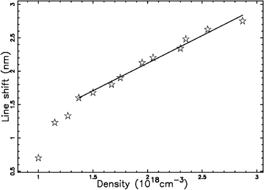
Figure 5: HgI 435.83 nm line shifts versus the electron density, data as extracted by the author from Figure 7 in [35] (empty stars) and linear regime (full line).

5 Two analytical models

The two mechanisms for the redshift here considered require the evaluation of the averaged density of electrons along the line of sight, which can be computed by

$$<n_{e}>\;=\frac{\int_{0}^{D}n_{e}(x)dx}{D}\quad,$$ (21)

where $D$ is the considered distance. This will be called the fundamental integral. We now present two models which are built in spherical symmetry.

5.1 The rim model

The radius of the cosmic voids as given by the Sloan Digital Sky Survey (SDSS) R7, has been modeled by spheres which have averaged radius $\bar{R}=\frac{18.23}{h}$ Mpc, see [36]. This means that the galaxies are situated on the thick surface of spheres having thickness $t$ much smaller than the averaged radius. We now suggest that the density of the free electrons follows the previous trend, and therefore

$$n_{e}(r)=n_{0} if \quad\,0\,\leq\,r\,<a$$

$$n_{e}(r)=n_{1} if \quad\,a\,\leq\,r\,<b$$ (22)

$$n_{e}(r)=n_{0} if \quad\,r\geq b$$

where $r$ is the distance from the origin of a Cartesian 3D reference system. This means that the electron density rises from $n_{0}$ at the center of the sphere to $n_{1}$ at $r=a$, remains constant up to $r=b$ (the radius of the void), and then falls again to $n_{0}$ outside the sphere. The fundamental integral of the density as represented by Equation (21) can be done in the $x$-direction over the length $D=2b$ and is split into two parts,

part  I, three pieces if $$\quad\,0\,\leq\,y\,<a$$

part II, two pieces if $$\quad\,a\,\leq\,y\,<b$$

corresponding to the lines of sight $s_{1}$ and $s_{2}$ in Figure 6.

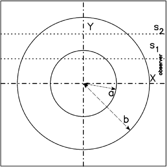
Figure 6: The two circles (sections of spheres) which include the region with an enhancement in electron density are represented by full lines. The observer is situated along the $x$ direction, and two lines of sight are indicated.

The result of the integral of the averaged electron density, see (21), is

$$<n_{e}>\;=\frac{n_{{0}}b-n_{{0}}\sqrt{{b}^{2}-{y}^{2}}+n_{{1}}\sqrt{{b}^{2}-{y}^{2}}-n_{{1}}\sqrt{{a}^{2}-{y}^{2}}+n_{{0}}\sqrt{{a}^{2}-{y}^{2}}}{b}$$

$$\mbox{if}\quad\,0\,\leq\,y\,<a$$

(23)

$$<n_{e}>\;=\frac{n_{{0}}b-n_{{0}}\sqrt{{b}^{2}-{y}^{2}}+n_{{1}}\sqrt{{b}^{2}-{y}^{2}}}{b}$$

$$\mbox{if}\quad\,a\,\leq\,y\,<b\quad.$$

The Hubble constant can be obtained from the averaged electron density by a multiplication with a numerical factor, see Equation (21) for the photo-absorption process. Figure 7 reports the behavior of Hubble’s constant as a function of the observer’s position and Table 2, the statistical parameters along the line of sight.

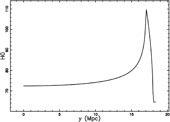
Figure 7: Value of $H_{0}$ for the photo-absorption process as function of the position; $b=18$ Mpc, $a=17$ Mpc, $n_{0}=5.1\,10^{-7}\mathrm{particles\,cm^{-3}}$, and $n_{1}=1.63\,10^{-6}\mathrm{particles\,cm^{-3}}$.

Table 2: The Hubble constant for the photo-absorption process.

entity	definition	value
$N$	No. of samples	200
$\bar{x}$	average	76.27 $\mathrm{km\,s^{-1}\,Mpc^{-1}}$
$\sigma$	standard deviation	7.16b $\mathrm{km\,s^{-1}\,Mpc^{-1}}$
$H_{0},max$	maximum	109.6 $\mathrm{km\,s^{-1}\,Mpc^{-1}}$
$H_{0},min$	minimum	64.51 $\mathrm{km\,s^{-1}\,Mpc^{-1}}$

5.2 The auto-gravitating model

We now present two solutions of two differential equations which can represent the physical basis of two different PDFs. On solving the fundamental hydrostatic equation for the magneto-hydrostatic model in the direction perpendicular to the galactic plane (the $x$-direction), the solution for the density is

$$\bar{\rho}(x)=\bar{\rho}(0)\exp{-(\frac{x}{H})^{2})}\quad,$$ (24)

where $\bar{\rho}(x)$ is the mean gas density and $H$ is the layer half-thickness, see equation (6.142) in [37]. The density profile of a thin self-gravitating disk of stars which is characterized by a Maxwellian distribution in velocity and a distribution which varies only in the $x$-direction is

$$n(x)=n_{0}sech^{2}(\frac{x}{2\,x_{0}})\quad,$$ (25)

where $n_{0}$ is the star density at $x=0$, $x_{0}$ is a scaling parameter, and sech is the hyperbolic secant, see formula (2.31) in ([38]). The physical solution represented by (24) becomes, when normalized, the Normal (Gaussian) distribution which has PDF

$$N(x;\sigma)=\frac{1}{\sigma(2\pi)^{1/2}}\exp({-{\frac{x^{2}}{2\sigma^{2}}}})\quad-\infty<x<\infty\quad.$$ (26)

The mean is

$$E(x;\sigma)=0\quad,$$ (27)

and the variance is

$$VAR(x;\sigma)=\sigma^{2}\quad.$$ (28)

The physical law represented by Equation (25) can be converted to a probability density function (PDF), the probability of having a given physical quantity at a distance between $x$ and $x+dx$,

$$p(x;x_{0})=\frac{1}{4}\,\left({\it sech}\left(\frac{1}{2}\,{\frac{\left|x\right|}{x_{{0}}}}\right)\right)^{2}\frac{1}{x_{0}}\quad.$$ (29)

The range of existence of this PDF is in the interval $[-\infty,\infty]$. The average value is $E(x;x_{0})=0$ and the variance is

$$VAR(x;x_{0})=\frac{1}{6}\,{x_{{0}}}^{2}{\pi}^{2}\quad.$$ (30)

This PDF can be transformed in such a way that it can be compared with the normal (Gaussian) as represented by Equation 26. The substitution $x_{0}={\frac{\sqrt{3}\sigma}{\pi}}$ transforms the PDF (29) into

$$p(x;\sigma)=\frac{1}{12}\,\left({\it sech}\left(\frac{1}{6}\,{\frac{\left|x\right|\pi\,\sqrt{3}}{\sigma}}\right)\right)^{2}\pi\,\sqrt{3}\frac{1}{\sigma}\quad.$$ (31)

The average value is $E(x;\sigma)=0$ and the variance is

$$VAR(x;\sigma)=\sigma^{2}\quad.$$ (32)

This PDF is referred to as the logistic function, see [39, 40, 41]. The similarity with the normal distribution is straightforward and Figure 8 reports the two PDFs when the value of $\sigma$ is equal in both cases.

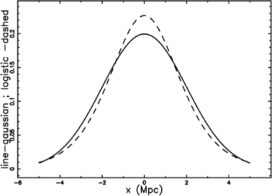
Figure 8: Normal PDF (full line) and logistic as represented by Eq. (31) (dashed line) when $\sigma=2{\mbox{Mpc}}/h$.

We now assume that the radial density of the free electrons follows the logistic law as given by Equation (8), in which $x$ is now the distance from the surface of the sphere. This assumption can be made when $\sigma\ll\bar{R}$. In order to deal with distances from the spherical surfaces greater than $\sigma$, where the density is supposed to be constant, the following three-part density function is suggested.

$$n_{e}(r)=n_{0} if \quad\,0\,\leq\,r\,<a$$

$$n_{e}(r)=n_{{0}}\frac{\left({\it sech}\left(1/6\,{\frac{\left(r-b\right)\pi\,\sqrt{3}}{\sigma}}\right)\right)^{2}}{\left({\it sech}\left(0.9068\,n\right)\right)^{2}} if \quad\,a\,\leq\,r\,<c$$ (33)

$$n_{e}(r)=n_{0} if \quad\,r\geq c.$$

Here, $r$ is the distance from the origin of a Cartesian 3D reference system. In order to avoid an increase in the number of parameters, $a$ and $c$ can be parametrized with the distance $n\,\sigma$ after which the density is constant,

$$a=b-n\sigma\qquad c=b+n\sigma\quad,$$ (34)

where $n$ is an integer. A simple evaluation says that the maximum density is reached at $r=b$, where the density is

$$n_{e}(r)={\frac{{\it n_{0}}}{\left({\it sech}\left(0.9068\,n\right)\right)^{2}}}\quad.$$ (35)

This profile density , see Equation (5.2), as a function of the distance from the center of the void, is shown in Figure 9.

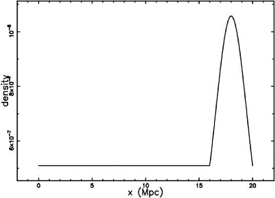
Figure 9: Profile of the three-part density function of free electrons as a function of the distance from the center of the void; $n_{0}=5\,10^{-7}\mathrm{particles\,cm^{-3}}$ , $n=2$, $b=18\,\mbox{Mpc}/h$, $\sigma=2$ Mpc/$h$.

We insert, into the three-part density profile of the free electrons, $r=\sqrt{x^{2}+y^{2}}$ and perform the integration of (21) over $x$ maintaining $y$ constant. An analytical expression for the integral does not exist, and the numerical integration, (using Boole’s rule, see [42], gives the averaged density. Under the hypothesis of the photo-absorption process, see Equation (21), Figure 10 presents the behavior of Hubble’s constant as a function of the observer’s position and Table 3, the statistical parameters along the line of sight.

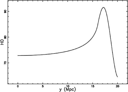
Figure 10: Value of $H_{0}$ for the photo-absorption process as a function of the position in the three-part density of the free electrons; $b=18$ Mpc, $s=2$ Mpc, $n=1$ Mpc, and $n_{0}=5.1\,10^{-7}\mathrm{particles\,cm^{-3}}$.

Table 3: The Hubble constant for the photo-absorption process with a three-part density of free electrons.

entity	definition	value
$N$	No. of samples	200
$\bar{x}$	average	76.25 $\mathrm{km\,s^{-1}\,Mpc^{-1}}$
$\sigma$	standard deviation	5.48 $\mathrm{km\,s^{-1}\,Mpc^{-1}}$
$H_{0},max$	maximum	91.56 $\mathrm{km\,s^{-1}\,Mpc^{-1}}$
$H_{0},min$	minimum	64.51 $\mathrm{km\,s^{-1}\,Mpc^{-1}}$

6 A theoretical model

A possible model for the spatial distribution of galaxies is represented by the Voronoi diagrams, but two requirements should be satisfied. The first is that the average radius of the voids be $<R>=18.23h^{-1}$ Mpc, which is the effective radius in SDSS DR7, see Table 6 in [43]. The second requirement is connected to the fact that the effective radius of the cosmic voids as deduced from catalog SDSS R7 is represented by a Kiang function with $c\approx 2$. This means that we are considering a non-Poissonian Voronoi Tessellation (NPVT). The density of free electrons can be found: (i) computing the distance $d$ of a 3D grid point from the nearest face, (ii) inserting such a distance in the following two-part density

$$n_{e}(d)=n_{{0}}\frac{\left({\it sech}\left(1/6\,{\frac{d\pi\,\sqrt{3}}{\sigma}}\right)\right)^{2}}{\left({\it sech}\left(0.9068\,n\right)\right)^{2}} if \quad\,d\,<c$$

$$n_{e}(d)=n_{0} if \quad\,d\geq c$$

with $c=n\,\sigma$. Given a cubic box of size 100 Mpc, Figure 11 shows the contour plots of the Hubble constant when a plane crossing the center is considered, and Table 4 gives the statistics. In this case, the fundamental integral of the density as represented by Equation (21) is evaluated numerically along lines belonging to the selected plane.

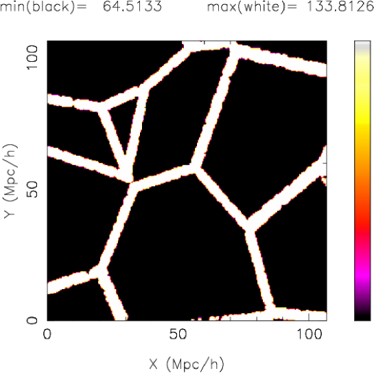
Figure 11: Contour plot of $H_{0}$ for the photo-absorption process as a function of the position in a 2D cut; $\sigma=1.9$ Mpc, $n_{0}=5.1\,10^{-7}\mathrm{particles\,cm^{-3}}$ and $n=1$.

Table 4: The Hubble constant for the photo-absorption process in the 2D cut of a Voronoi diagram.

entity	definition	value
$N$	No. of samples	301
$\bar{x}$	average	76.45 $\mathrm{km\,s^{-1}\,Mpc^{-1}}$
$\sigma$	standard deviation	6.11 $\mathrm{km\,s^{-1}\,Mpc^{-1}}$
$H_{0},max$	maximum	96.51 $\mathrm{km\,s^{-1}\,Mpc^{-1}}$
$H_{0},min$	minimum	68.88 $\mathrm{km\,s^{-1}\,Mpc^{-1}}$

The fundamental integral (21) which gives the averaged density can be done also along an arbitrary line characterized by a given galactic latitude and longitude. Figure 12 shows the contours of the Hubble constant on the surface of a sphere using the the subroutine GLOBE which belongs to the package PGXTAL.

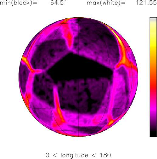
Figure 12: Contour plot of $H_{0}$ on the surface of a sphere, parameters as in Figure 11.

7 The astronomer’s model

We analyze the 3D spatial distribution of galaxies given by the 2MASS Redshift Survey (2MRS), see Figure 13.

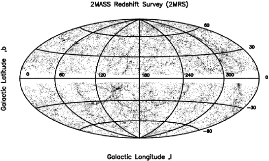
Figure 13: Hammer–Aitoff projection in galactic coordinates of the 2MRS galaxies when $z\leq 0.04$.

An updated real 3D distribution of galaxies as given by the 2MRS catalog is the first ingredient of the astronomer’s model. The self-gravitating sphere of polytropic gas is regulated by the Lane–Emden differential equation of the second order,

$${\frac{d^{2}}{d{x}^{2}}}Y\left(x\right)+2\,{\frac{{\frac{d}{dx}}Y\left(x\right)}{x}}+\left(Y\left(x\right)\right)^{n}=0\quad,$$ (37)

where $n$ is an integer, see [44, 45, 46, 47, 48].

The solution $Y\left(x\right)_{n}$ produces the density profile

$$\rho=\rho_{c}Y\left(x\right)_{n}^{n}\quad,$$ (38)

where $\rho_{c}$ is the density at $x=0$.

Analytical solutions exist for $n=0,1$, and 5. The analytical solution for $n=0$ is

$$Y(x)=\frac{sin(x)}{x}\quad,$$ (39)

and has therefore an oscillatory behavior. The analytical solution for $n=5$ is

$$Y(x)={\frac{1}{{(1+\frac{{x}^{2}}{3})^{1/2}}}}\quad,$$ (40)

and the density for $n=5$ is

$$\rho(x)=\rho_{c}{\frac{1}{{(1+\frac{{x}^{2}}{3})^{5/2}}}}\quad.$$ (41)

The asymptotic behavior for large values of $x$ of the density when $n=5$ is

$$\rho(x)=9\,{\frac{\sqrt{3}}{{x}^{5}}}+O\left(\frac{1}{x^{7}}\right)\quad.$$ (42)

On introducing the scale , $b$, and normalizing the function (41), we obtain the Lane–Emden5 (i.e., $n=5$) PDF, LE5,

$$LE5(x;b)=\frac{\sqrt{3}}{2\,\left(1+\frac{1}{3}\,{\frac{{y}^{2}}{{b}^{2}}}\right)^{5/2}b}\quad,$$ (43)

which has average value

$$E(x;b)=\frac{1}{2}\,\sqrt{3}b\quad,$$ (44)

and variance

$$VAR(x;b)=\frac{3}{4}\,{b}^{2}\quad.$$ (45)

The density $\rho$ can be written as $\rho(x)=n(x)m_{H}$ where $m_{H}$ is the mass of hydrogen. On assuming the neutrality of the charges, the number density of the electrons is

$$n_{e}(x)=n_{c}LE5(x;b)\quad,$$ (46)

where $n_{c}$ is the central number density of the electrons. We now assume that the Lane–Emden profile can be applied from $x=0$ to a given value of $x$ after which the number density is decreased by a given factor $f$. After this length, the number density of electrons has a constant value $n(x)=n_{0}$, where $n_{0}$ is a constant. The inequality which fixes the previous assumption is

$$\cases{n_{e}(x)=f{\it n_{0}}\left(1+1/3\,{\frac{{x}^{2}}{{b}^{2}}}\right)^{-5/2}&when \, $0<x<\sqrt{-3+3\,{f}^{2/5}}b$\cr{\it n_{e}(x)=n_{0}}&when \, $x>\sqrt{-3+3\,{f}^{2/5}}$.\cr}$$ (47)

A typical example with the parameters that will be used in the forthcoming simulation is given in Figure 14.

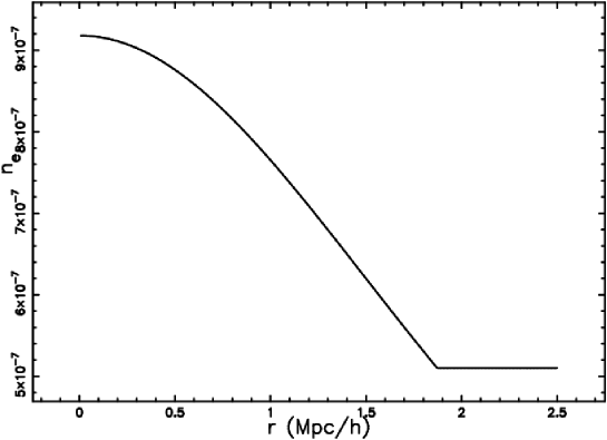
Figure 14: Profile of density of free electrons as a function of the distance from the center of the void; $n_{0}=5.1\,10^{-7}\mathrm{particles\,cm^{-3}}$ , $b=2.55$ Mpc/$h$, $f=2.35$ .

The radial distribution of electrons as given by the Lane–Emden ($n=5$) profile is the second ingredient of the astronomer’s model. Figures 15, respectively, 16, give the contours of the Hubble constant on the surface of the first, respectively, second, half-sky where the fundamental integral (21) which gives the averaged density has been used. The contours of the Hubble constant can also be drawn in the Aitoff–Hammer projection, see Figure 17, and Table 5 gives the statistics of the Hubble constant.

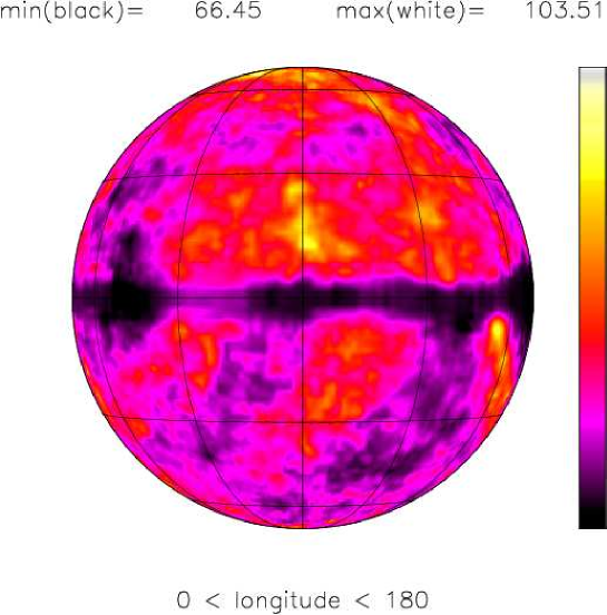
Figure 15: Contour plot of $H_{0}$ as given by the astronomer’s model on the surface of a sphere, parameters as in Figure 14. Galactic longitude between 0^∘ and 180^∘.

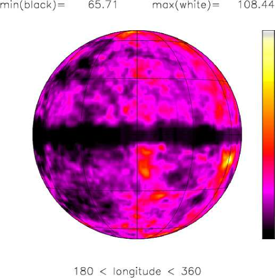
Figure 16: Contour plot of $H_{0}$ as given by the astronomer’s model on the surface of a sphere, parameters as in Figure 14. Galactic longitude between 180^∘ and 360^∘.

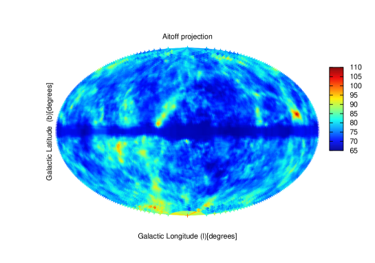
Figure 17: False color contour plot of $H_{0}$ as given by the astronomer’s model in the Aitoff–Hammer equal-area map in galactic coordinates with the Galactic center in the middle, parameters as in Figure 14.

Table 5: The Hubble constant for the photo-absorption process in the astronomer’s model.

entity	definition	value
$n$	No. of samples	16471
$\bar{x}$	average	76.1 $\mathrm{km\,s^{-1}\,Mpc^{-1}}$
$\sigma$	standard deviation	5.5 $\mathrm{km\,s^{-1}\,Mpc^{-1}}$
$H_{0},max$	maximum	105.91 $\mathrm{km\,s^{-1}\,Mpc^{-1}}$
$H_{0},min$	minimum	65.69 $\mathrm{km\,s^{-1}\,Mpc^{-1}}$

8 Conclusions

The fact that the recent observations of galaxies reveal a cellular structure as opposed to a homogeneous structure, see Section 3, allows exploring a definition of the Hubble constant outside of the standard cosmology. We therefore explained the anisotropies in the Hubble constant by variations in the number of electrons on the line of sight in the framework of the photo-absorption process. The observed average value and variance in the all sky measures have been reproduced in the analytical, simulated, and astronomer’s models, see Tables 2, 3, 4, and 5. The statistical deviations of the Hubble constant are high and the standard uncertainty is 10.57 $\mathrm{km\,s^{-1}\,Mpc^{-1}}$, which means a relative standard uncertainty of 0.13, see Table 1. We have reproduced this high statistical fluctuation and the relative standard uncertainty is 0.0938 and 0.0718 for the two analytical models, see Tables 2 and 3, 0.079 for the simulated model, see Table 4, and 0.072 for the astronomer’s model, see Table 5.

References

- [1] E. Hubble, A Relation between Distance and Radial Velocity among Extra-Galactic Nebulae, Proceedings of the National Academy of Science 15 (1929), 168–173.
- [2] W. L. Freedman, B. F. Madore, V. Scowcroft, C. Burns, A. Monson, S. E. Persson, M. Seibert, J. Rigby, Carnegie Hubble Program: A Mid-infrared Calibration of the Hubble Constant, ApJ 758 (2012), 24.
- [3] P. J. Mohr, B. N. Taylor, D. B. Newell, CODATA recommended values of the fundamental physical constants: 2010, Reviews of Modern Physics 84 (2012), 1527–1605.
- [4] A. Friedmann, Über die Krümmung des Raumes, Zeitschrift fur Physik 10 (1922), 377–386.
- [5] A. Friedmann, Über die möglichkeit einer welt mit konstanter negativer krümmung des raumes, Zeitschrift für Physik A Hadrons and Nuclei 21 (1) (1924), 326–332.
- [6] A. G. Riess, A. V. Filippenko, P. Challis, A. Clocchiatti, Observational Evidence from Supernovae for an Accelerating Universe and a Cosmological Constant, AJ 116 (1998), 1009–1038.
- [7] S. Perlmutter, G. Aldering, G. Goldhaber, R. A. Knop, Measurements of Omega and Lambda from 42 High-Redshift Supernovae, ApJ 517 (1999), 565–586.
- [8] F. Zwicky, On the Red Shift of Spectral Lines through Interstellar Space, Proceedings of the National Academy of Science 15 (1929), 773–779.
- [9] A. Brynjolfsson, Redshift of photons penetrating a hot plasma, arXiv:astro-ph/0401420 .
- [10] A. Brynjolfsson, Plasma-Redshift Cosmology: A Review, in: F. Potter (Ed.), Astronomical Society of the Pacific Conference Series, Vol. 413, 2009, 169–189.
- [11] L. Ashmore, Recoil between photons and electrons leading to the Hubble constant and CMB, Galilean Electrodynamics 17 (3) (2006), 53.
- [12] D. F. Crawford, Curvature Cosmology, Brown Walker, Boca Raton, FL, USA, 2006.
- [13] D. F. Crawford, Observational Evidence Favors a Static Universe (Part I), Journal of Cosmology 13 (2011), 3875–3946.
- [14] D. L. Mamas, An explanation for the cosmological redshift, Physics Essays 23 (2010), 326.
- [15] M. Michelini, The new cosmology rising from the quantum pushing gravity interaction—The case of accelerating universe, Applied Physics Research 5 (5) (2013), 67–84.
- [16] L. Marmet, Survey of Redshift Relationships for the Proposed Mechanisms at the 2^nd Crisis in Cosmology Conference, in: F. Potter (Ed.), Astronomical Society of the Pacific Conference Series, Vol. 413, 2009, 315–335.
- [17] H. Karoji, M. Moles, Markarian galaxies and the angular anisotropy of the Hubble ‘constant’, Academie des Sciences Paris Comptes Rendus Serie B Sciences Physiques 280 (1975), 609–612.
- [18] B. N. G. Guthrie, Anisotropy in the Hubble Relation for the Brightest Galaxies in Clusters, Astrophysics and Space Science 43 (1976), 425–431.
- [19] A. J. Fennelly, Anisotropy in the Hubble parameter and large-scale cosmological inhomogeneity, MNRAS 181 (1977), 121–130.
- [20] D. L. Wiltshire, P. R. Smale, T. Mattsson, R. Watkins, Hubble flow variance and the cosmic rest frame, Phys. Rev. D 88 (8) (2013), 083529.
- [21] A. Einstein, Die Grundlage der allgemeinen Relativitätstheorie, Annalen der Physik 354 (1916), 769–822.
- [22] A. Einstein, Kosmologische Betrachtungen zur allgemeinen Relativitätstheorie, Sitzungsberichte der Königlich Preußischen Akademie der Wissenschaften (Berlin), (1917), 142–152.
- [23] A. Einstein, Bemerkung zu der Franz Seletyschen arbeit—Beiträge zum kosmologischen system, Annalen der Physik 374 (1922), 436–438.
- [24] F. Wang, Physics with MAPLE: The Computer Algebra Resource for Mathematical Methods in Physics, Wiley-VCH, New York, 2006.
- [25] M. L. McClure, C. C. Dyer, Anisotropy in the Hubble constant as observed in the HST extragalactic distance scale key project results, New Astronomy 12 (2007), 533–543.
- [26] W. R. Leo, Techniques for Nuclear and Particle Physics Experiments, Springer-Verlag, Berlin, 1994.
- [27] L. Zaninetti, New formulas for the Hubble constant in a Euclidean static universe, Physics Essays 23 (2010), 298–307.
- [28] P. Marmet, A new non-Doppler redshift, Physics Essays 1 (1) (1988), 24–32.
- [29] H. Nguyen, M. Koenig, D. Benredjem, M. Caby, G. Coulaud, Atomic structure and polarization line shift in dense and hot plasmas, Phys. Rev. A 33 (1986), 1279–1290.
- [30] Y. Leng, J. Goldhar, H. R. Griem, R. W. Lee, C vi Lyman line profiles from 10-ps KrF-laser-produced plasmas, Phys. Rev. E 52 (1995), 4328–4337.
- [31] A. Saemann, K. Eidmann, I. E. Golovkin, Isochoric heating of solid aluminum by ultrashort laser pulses focused on a tamped target, Physical Review Letters 82 (24) (1999), 4843–4846.
- [32] A. G. Zhidkov, A. Sasaki, T. Tajima, Direct spectroscopic observation of multiple-charged-ion acceleration by an intense femtosecond-pulse laser, Physical Review E 60 (3) (1999), 3273–3278.
- [33] H. Wang, X. Yang, X. Li, Ground-State Energy Shifts of H-Like Ti Under Dense and Hot Plasma Conditions, Plasma Science and Technology 9 (2007), 128–132.
- [34] L. Ashmore, Intrinsic plasma redshifts now reproduced in the laboratory—A discussion in terms of new tired light. viXra:Astrophysics:1105.0010 .
- [35] C. S. Chen, X. L. Zhou, B. Y. Man, Y. Q. Zhang, J. Guo, Investigation of the mechanism of spectral emission and redshifts of atomic line in laser-induced plasmas, Optik 120 (2009), 473–478.
- [36] D. C. Pan, M. S. Vogeley, F. Hoyle, Y.-Y. Choi, C. Park, Cosmic voids in Sloan Digital Sky Survey Data Release 7, MNRAS 421 (2012), 926–934.
- [37] H. Scheffler, H. Elsaesser, Physics of the galaxy and interstellar matter, Springer-Verlag, Berlin, 1987.
- [38] P. Padmanabhan, Theoretical astrophysics. Vol. III: Galaxies and Cosmology, Cambridge University Press, 2002.
- [39] N. Balakrishnan, Handbook of the Logistic Distribution, Taylor & Francis, New York, 1991.
- [40] N. L. Johnson, S. Kotz, N. Balakrishnan, Continuous univariate distributions. Vol. 2. 2nd ed., Wiley, New York, 1995.
- [41] M. Evans, N. Hastings, B. Peacock, Statistical Distributions, 3rd. ed., Wiley, New York, 2000.
- [42] M. Abramowitz, I. A. Stegun, Handbook of Mathematical Functions with Formulas, Graphs, and Mathematical Tables, Dover, New York, 1965.
- [43] L. Zaninetti, New Analytical Results for Poissonian and non-Poissonian Statistics of Cosmic Voids, Revista Mexicana de Astronomia y Astrofisica 48 (2012), 209–222.
- [44] H. J. Lane, On the theoretical temperature of the sun, under the hypothesis of a gaseous mass maintaining its volume by its internal heat, and depending on the laws of gases as known to terrestrial experiment, American Journal of Science (148) (1870), 57–74.
- [45] R. Emden, Gaskugeln: Anwendungen der mechanischen Wärmetheorie auf kosmologische und meteorologische Probleme, Teubner, Berlin, 1907.
- [46] S. Chandrasekhar, An Introduction to the Study of Stellar Structure, New York, 1967.
- [47] J. Binney, S. Tremaine, Galactic Dynamics, Princeton University Press, 1987.
- [48] D. Zwillinger, Handbook of Differential Equations, Academic Press, New York, 1989.