Fermionization, Triangularization and Integrability

Abstract

In this article, we derive the fermionic formalism of Hamiltonians as well as corresponding excitation spectrums and states of Calogero-Sutherland(CS), Laughlin and Halperin systems, respectively. In addition, we study the triangular property of these Hamiltonians and prove the integrability in these three cases.

1 Introduction and Results

In the area of many body physics, fractional quantum Hall effects (FQHEs) and integrable models, are two fruitful and important classes. Many researchers believe these two are connected in a hundred and one ways. [1, 2, 5, 10, 14, 30, 31] Plenty of efforts have been dedicated to find out the intrinsic relationship.

In FQHEs, the Laughlin trial wavefunction reveals several remarkable properties of FQHEs at filling number $\nu=\frac{1}{2m+1},$ such as the fractional statistics as well as the topological orders. Later on a conformal field theory (CFT) realization was discovered which shows that the wavefunction is corresponding to a correlation function of certain vertex operators . Furthermore this idea is generalized to many other FQH states, e.g. Halperin state[16], Moore-Read state, and Read-Rezayi state[24], et.al[3, 13, 21, 28]. However, CFT is possibly not sufficient to drive the dynamics of the edge theory, since it only determines the behavior of the theory near critical point..

A more ambitious thinking is to find the Hamiltonian system behind the edge ground state. So far, there are two classes of Hamiltonian analysis for FQHE. One is the Chern-Simons approach, initiated by Zhang, Hansson and Kivelson in 1989[30]. The other is the extended Hamiltonian theory, introduced by Murthy and Shankar in late 90’s[22, 23, 25]. The later one contains Chern-Simons as its asymptotic theory.

In our study we try to approach the integrability problem in a different way. In fact, we are not meant to establish a unified Hamiltonian theory to solve the complicated many-body problem. Instead we are looking for the integrability behind FQHEs as well as the Hamiltonian expression of it. In order to do so we separate the excitations of FQHE into two simple classes: the perturbative class and nonperturbative one. The nonperturbative class dominates the states in Hilbert space, a.k.a. the basis, the perturbative class organizes those basis into physical states. So perturbations actually are provided as structure constants (or superposition coefficients). Interestingly, this idea is like in CFT, where correlation function is made by conformal block and structure constant (it encodes the multiplicity of the corresponding conformal block in the correlation function. ) Since the ground state should not change by perturbations it belongs to the nonperturbative class. Hence it describes a sort of wave without dissipation which implies that the ground state is a solitonic wave.

In this way we have related the FQHE theory to soliton theory, the other important area of many-body physics. The question now is to extract excitations from the solitonic wavefunction. The stable excitations from the soliton wavefunction, are those solutions of quantum mechanics equation for soliton wave[7]. In this quantum mechanics, the logarithmic of the soliton wavefunction is a scalar function, while its gradation, gives the effective “gauge” potential. Therefore, the Hamiltonian could be written as a Landau-Ginzberg pseudo-potential form.

Inspired by these observations and a previous work [29], we use the same method for Laughlin and Halperin states. Then we obtain complicated Hamiltonians with non-linear interactions. However, they are all exact solvable. The resolving strategy is as follows: firstly, we interpret the ground state as correlation function in CFT. Secondly, by Jastrow transformation we drop the contribution of ground state and obtain a relative simple Hamiltonian. Thirdly, the eigen-equation of the new Hamiltonian can be transformed into an operator equation acting on the coherent basis. Fourthly, it turns out that the operator formalism is exactly triangulated. Therefore we can extract the spectrum as well as the state in a recursive way. Finally, to analyze the integrability closely, we derive the fermionization for the bosonic theory. Hence the integrability is clearly determined by free fermions and the explicit triangularization.

We find, interestingly, the integrability behind Laughlin state, is the same as the famous Calogero-Sutherland model. Hence the excitations are those of Jack polynomials[20]. During last two decades, people claimed that ground states of some FQHEs have the same properties as those of Jack polynomials. For example the $(k,r,N)$-admissible representations (labeled by certain restricted Young diagrams) is related to the filling number $\nu=\frac{k}{r}$ FQHE ground state[1, 4, 6, 8, 9, 11, 12, 14, 17, 19]. From our viewpoint the basic ingredients are Jack polynomials and additional restrictions, mostly from the fusion rule (which we do not explore in this article), will rule out some Jack polynomials systematically which results in the admissible representations.

The Halperin state, corresponding to the two-layer FQHE, shows a secret integrability dominated by also the triangularization, which says the number of boxes in Young diagram for the first layer always decreases while the one for the second layer increases and the total boxes of these two layers remain the same. The triangularization interaction, being triple in two kinds of bosonic operators, is quite complicated. It makes the explicit solution of the excitations slightly difficult. Nevertheless, since the triangularization is clear, we can give the explicit solution of the system in principle.

This article is organized as follows. In sec. 2, we review the famous Calogero-Sutherland model, its operator formalism, the CFT correspondence, the spectrum and eigenstates. In sec. 3 we obtain the fermionization of the CS theory followed by the fermionic triangularization and integrability. In sec. 4 and 5, we provide parallel analysis for Laughlin state and Halperin state. In sec. 6 we make a conclusion and discuss some further works.

2 The Calogero-Sutherland Model

We start our analysis from the famous Calogero-Sutherland(CS) model. It is an exact solvable model, describing $N$ interacting charged particles on a unit circle, with two-body interaction

$$H_{int}=\sum_{i<j} \frac{\beta(\beta-1)}{\sin^{2}(x_{i}-x_{j})} \,,$$

in which $x_{i}$ defines the $i$-th particle’s position on the circle. For simplicity, we substitute $\beta=b^{2}$. Then CS Hamiltonian is written as

$$H_{CS}=-\frac{1}{2}\sum_{i=1}^{N}\partial_{i}^{2}+\sum_{i<j}\frac{b^{2}(b^{2}-1)}{\sin^{2}(x_{i}-x_{j})}\,.$$ (1)

Theorem 1.

$H_{CS}$ is isospectral to another Hamiltonian

$$\tilde{H}_{CS}=-\frac{1}{2}\sum_{i=1}^{N}(\partial_{i}+\partial_{i}\ln\prod_{j<k}\sin^{b^{2}}(x_{j}-x_{k}))(\partial_{i}-\partial_{i}\ln\prod_{r<s}\sin^{b^{2}}(x_{r}-x_{s})\,.$$ (2)

up to a universal shift of eigen-energy.

Proof of Theorem 1: Defining the complex coordinate $z_{i}=e^{i2x_{i}}$, we have $\partial_{i}=2iz_{i}\partial_{z_{i}}$. Therefore

$$\partial_{i}\ln\prod_{j<k}\sin^{b^{2}}(x_{j}-x_{k}) = b^{2}\sum_{\begin{subarray}{c}j\\ i\neq j\end{subarray}}\cot(x_{i}-x_{j})$$

$$= ib^{2}\sum_{\begin{subarray}{c}j\\ i\neq j\end{subarray}}\frac{z_{i}+z_{j}}{z_{i}-z_{j}}\,,$$

and the commutator

$$\left[\partial_{i},b^{2}\sum_{\begin{subarray}{c}k\\ i\neq k\end{subarray}}\cot(x_{i}-x_{k})\right]=-b^{2}\sum_{\begin{subarray}{c}k\\ k\neq i\end{subarray}}\frac{1}{\sin^{2}(x_{k}-x_{i})}.$$

We can rewrite the $\tilde{H}_{CS}$ as the following formula

$$\tilde{H}_{CS} = -\frac{1}{2}\sum_{i=1}^{N}\partial_{i}^{2}-b^{2}\sum_{i<j}\frac{1}{\sin^{2}(x_{i}-x_{j})}$$

$$+\frac{1}{2}b^{4}\sum_{i\neq j,i\neq k}\cot\left(x_{i}-x_{j}\right)\cot\left(x_{i}-x_{k}\right)\,.$$

Using the identity

$$\sum_{\hbox{distinct \ }i,j,k}\cot\left(x_{i}-x_{j}\right)\cot\left(x_{i}-x_{k}\right)+{i,j,k}\text{{\ cyclic}}$$

$$=\sum_{\hbox{distinct\ }i,j,k}(-1)=-N(N-1)(N-2) \,,$$

and the $j=k$ contribution

$$\sum_{i\neq j}\cot^{2}\left(x_{i}-x_{j}\right)=-\sum_{i\neq j}1+\sum_{i\neq j}\frac{1}{\sin^{2}(x_{i}-x_{j})}\,,$$

we now have the form of $\tilde{H}_{CS}$ as

$$\tilde{H}_{CS} = -\frac{1}{2}\sum_{i=1}^{N}\partial_{i}^{2}+b^{2}(b^{2}-1)\sum_{i<j}\frac{1}{\sin^{2}(x_{i}-x_{j})}-\frac{1}{6}b^{4}(N-1)N(N+1)\,,$$ (3)

$$= H_{CS}-\frac{1}{6}b^{4}N(N-1)(N+1)$$

so Theorem 1 is proved. Q.E.D.

It is now nature to consider the $\tilde{H}_{CS}$ rather than $H_{CS}$ since the later one, when acting on the ground state, will have a large energy (proportional to $N^{3}$) contribution to the spectrum. The ground state of $\tilde{H}_{CS}$ is simply

$$\Psi_{CS}=\prod_{i<j}\sin^{\beta}(x_{i}-x_{j}),\quad\tilde{H}_{CS}\Psi_{CS}=0\text{\,.}$$ (4)

To extract the spectrums as well as corresponding excitation states, we need to eliminate the contribution of ground state. It implies the Jacobi transformation

$$2H^{\prime}_{CS}=\Psi_{CS}^{-1}\tilde{H}_{CS}\Psi_{CS}\,.$$

In this way, we have

$$2H^{\prime}_{CS} = -\frac{1}{2}\sum_{i}(\partial_{i}+2\partial_{i}\ln\Psi_{CS})\partial_{i}$$ (5)

$$= -\frac{1}{2}\sum_{i}(2iz_{i}\partial_{z_{i}}+i2b^{2}\sum_{i\neq j}\frac{z_{i}+z_{j}}{z_{i}-z_{j}})(2iz_{i}\partial_{z_{i}})$$

$$= 2\sum_{i}(z_{i}\partial_{z_{i}})^{2}+2b^{2}\sum_{i<j}\frac{z_{i}+z_{j}}{z_{i}-z_{j}}(z_{i}\partial_{z_{i}}-z_{j}\partial_{z_{j}})\,.$$

2.1 Bosonic oscillator formalism of $H^{\prime}_{CS}$

The ground state as in (4) can be understood as a CFT correlation function, that is

$$\Psi_{CS}({z_{i}})\simeq\langle k_{f}|\prod_{i=1}^{N}V_{b}(z_{i})|k_{in}\rangle\,,$$

with the vertex operator defined by

$$V_{b}(z)\equiv:e^{b\phi(z)}:\,,$$

and the bosonic field has the standard mode expansion

$$\phi(z) = q_{0}+p_{0}\ln z+\sum_{n\neq 0}\frac{a_{-n}}{n}z^{n}\,,$$

$${}[a_{n},a_{m}] = n\delta_{n+m,0},\quad[p_{0},q_{0}]=1\,.$$

We can show that briefly. The OPE of vertex operators reads

$$V_{a}(z)V_{b}(w)=(z-w)^{ab}:V_{a}V_{b}(\frac{z+w}{2}):\,.$$

If we choose the initial (final) momentum of right (left) vacuum $k_{in}=\frac{b}{2}(1-N)$ ($k_{f}=k_{in}+Nb$) , the correlation function is charge neutral and gives the result

$$\langle k_{f}|\prod_{i=1}^{N}V_{b}(z_{i})|k_{in}\rangle = \prod_{i<j}(z_{i}-z_{j})^{b^{2}}\prod_{i}(z_{i})^{\frac{b^{2}}{2}(1-N)}$$

$$= \prod_{i<j}\left(\frac{z_{i}-z_{j}}{\sqrt{z_{i}z_{j}}}\right)^{b^{2}}$$

$$= \prod_{i<j}(2i\sin(x_{i}-x_{j}))^{b^{2}}\,.$$

Therefore up to a constant factor, it is the ground state of CS model. The excitation state, in principle, will be a state in the Fock space of the conformal field theory, which in general is a polynomial of bosonic oscillators. It implies there are one-to-one correspondence from the excitation wavefunction to an oscillator polynomial. The basic relation is the coherent relation such that

$$a_{n}\prod_{i}V_{b}^{-}(z_{i})|k_{in}\rangle=b\sum_{i}z_{i}^{n}\prod_{i}V_{b}^{-}(z_{i})|k_{in}\rangle\,.$$ (6)

It relates the bosonic oscillator mode $a_{m}$to a symmetric polynomial (or symmetric function if $N\rightarrow\infty$). If we define the excitation state as follows

$$\frac{1}{2}\tilde{H}_{CS}\Psi_{\lambda}^{\beta}({z_{i}}) = \Psi_{CS}H^{\prime}_{CS}P_{\lambda}^{\beta}({z_{i}})=E_{\lambda}^{\beta}\Psi_{\lambda}^{\beta}({z_{i}})$$

$$\Psi_{\lambda}^{\beta}({z_{i}}) = \Psi_{CS}({z_{i}})P_{\lambda}^{\beta}({z_{i}})$$

$$\simeq \langle k_{f}|\prod_{i=1}^{N}V_{b}(z_{i})P_{\lambda}^{\beta}(a^{-})|k_{in}\rangle\,,$$

then

$$\langle k_{f}|P_{\lambda}^{\beta}(a^{+})H^{\prime}_{CS}(a)\prod_{i=1}^{N}V_{b}^{-}(z_{i})|k_{in}\rangle=E_{\lambda}^{\beta}P_{\lambda}^{\beta}({z_{i}})\,.$$ (7)

We have defined here the normal-ordered operator formalism of $H^{\prime}_{CS}(a)\equiv H$ , such that

$$H|P_{\lambda}^{\beta}\rangle=E_{\lambda}|P_{\lambda}^{\beta}\rangle.$$

The next step is to translate the differential formalism Hamiltonian $H^{\prime}_{CS}$ into operator formalism with the help of coherent relation (6). We have the following relations

$$z_{i}\partial_{z_{i}}\bullet=b\sum_{n>0}a_{-n}z_{i}^{n}\bullet, (z_{i}\partial_{z_{i}})^{2}\bullet=b^{2}\sum_{n,m>0}a_{-n}a_{-m}z_{i}^{n+m}\bullet+b\sum_{n>0}na_{-n}z_{i}^{n}\bullet$$

$$\sum_{i<j}\frac{z_{i}+z_{j}}{z_{i}-z_{j}}(z_{i}\partial_{z_{i}}-z_{j}\partial_{z_{j}})\bullet = b\sum_{i<j,n>0}a_{-n}\frac{z_{i}+z_{j}}{z_{i}-z_{j}}(z_{i}^{n}-z_{j}^{n})\bullet$$

$$=b\sum_{i<j,n>0}a_{-n}(z_{i}^{n}+2z_{i}^{n-1}z_{j} + \cdots 2z_{i}z_{j}^{n-1}+z_{j}^{n})\bullet$$

$$=\left(b\sum_{n,m>0,i,j}a_{-n}z_{i}^{n-m}z_{j}^{m}\right. + \left.Nb\sum_{n>0,i=1}^{N}a_{-n}z_{i}^{n}-b\sum_{n>0,i=1}^{N}na_{-n}z_{i}^{n}\right)\bullet$$

where $\bullet$ denotes $\prod_{j=1}^{N}V_{b}^{-}(z_{j})|k_{i}\rangle$. So we have the CS Hamiltonian in bosonic operator formalism

$$H=\sum_{n,m>0}b(a_{-n}a_{-m}a_{n+m}+a_{-n-m}a_{n}a_{m})$$ (8)

$$+(1-b^{2})\sum_{n>0}na_{-n}a_{n}+b^{2}N\sum_{n>0}a_{-n}a_{n}\,.$$

The last term involves the level of corresponding excitations, when $N\rightarrow\infty$, it overwhelms the excitation spectrum since it is much larger than other contributions in $H$. In our analysis, we treat it as the background and we ignore this term. Besides, if we set

$$\tilde{a}_{-n}=\frac{a_{-n}}{b},\,\,\tilde{a}_{n}=a_{n}b\,,{\text{f}or}\,\,n>0$$

then we rewrite $H$ as

$$H = \sum_{n,m>0}b(b\tilde{a}_{-n}\tilde{a}_{-m}\tilde{a}_{n+m}+\frac{1}{b}\tilde{a}_{-n-m}\tilde{a}_{n}\tilde{a}_{m})$$

$$+ (1-b^{2})\sum_{n>0}n\tilde{a}_{-n}\tilde{a}_{n}$$

$$= \sum_{n,m>0}(\tilde{a}_{-n}\tilde{a}_{-m}\tilde{a}_{n+m}+\tilde{a}_{-n-m}\tilde{a}_{n}\tilde{a}_{m})$$

$$+ (1-b^{2})\left(\sum_{n>0}n\tilde{a}_{-n}\tilde{a}_{n}-\sum_{n,m>0}\tilde{a}_{-n}\tilde{a}_{-m}\tilde{a}_{n+m}\right)\,.$$

It is easy to see that $\tilde{a}$ still holds the Heisenberg algebra so that the fermionization is exact. We split the Hamiltonian into free part (the first line of last equality of (2.1)), which is the same as free fermions, and the interacting part (the second line of last equality of (2.1)).

2.2 Eigenstate and spectrum

The CS model is exactly solvable. To see that, we first classify the Fock space expanded by bosons by its level $\mathcal{N}=\sum_{n>0}a_{-n}a_{n}$ such that an arbitrary state

$$|n_{1},n_{2},\cdots,n_{l}\rangle=a_{-n_{1}}a_{-n_{2}}\cdots\,a_{-n_{l}}|0\rangle\,,$$ (10)

has a level

$$\mathcal{N}|n_{1},n_{2},\cdots\,n_{l}\rangle=\sum_{i=1}^{l}n_{i}|n_{1},n_{2},\cdots\,n_{l}\rangle\,.$$

In this classification, there are $P(k)$, the partition number of $k$, states at a given level $k$. It is easy to check that $H$ commutes with $\mathcal{N}$. Hence they can have common eigenstates. Therefore, the eigenstate of $H$ can be obtained by a superposition of states like (10). A closer observation shows that the Hamiltonian $H$ acting on a state (10) at level $k$ by certain times will definitely generate the lowest state $|1^{k}\rangle\equiv(a_{-1})^{k}|0\rangle$. We can choose the coefficients of the Fock state $|1^{k}\rangle$ of all states at level $k$ to be the same and equal to $b^{-k}$. By this choice, we have removed the irrelevant c-number common factor of each eigenstate. For example, at level 4, we assume an eigenstate has the following formalism

$$|P_{\lambda}^{\beta}\rangle=b^{-4}((a_{-1})^{4}+\alpha_{1}a_{-2}(a_{-1})^{2}+\alpha_{2}a_{-2}^{2}+\alpha_{3}a_{-3}a_{-1}+\alpha_{4}a_{-4})|0\rangle\,,$$

Thus there are $P(4)-1=5-1=4$ unknown coefficients and also the eigen-energy $E_{\lambda}^{\beta}$ is not known. However, compare all the coefficients of the eigen-equation

$$H|P_{\lambda}^{\beta}\rangle=E_{\lambda}^{\beta}|P_{\lambda}^{\beta}\rangle\,,$$

we have in total 5 independent equations. They in turn determine the eigenstate completely. The generalization to level $k$ is then straightforward.

However, this method does not provide a clear relation between the eigenstate and the Young diagram underlining the theory. In general, one can define by hand a sequence of eigen-energies at a given level so that each state is uniquely related to a Young diagram. But the reason is weak and unnatural. However, it is quite natural to see the Young diagram from the fermionic picture, which we will explore in next section.

3 Fermionization

3.1 Fermionization of free term

We now rewrite the CS Hamiltonian as $H\equiv H_{0}+H_{int}$, here

$$H_{0}=\sum_{n,m>0}(\tilde{a}_{-n}\tilde{a}_{-m}\tilde{a}_{n+m}+\tilde{a}_{-n-m}\tilde{a}_{n}\tilde{a}_{m})$$ (11)

is the free part, while

$$H_{int}=(1-b^{2})\left(\sum_{n>0}n\tilde{a}_{-n}\tilde{a}_{n}-\sum_{n,m>0}\tilde{a}_{-n}\tilde{a}_{-m}\tilde{a}_{n+m}\right)$$ (12)

is the interaction part which could be separated into two components

$$H_{i}nt = H_{1}+H_{2},H_{1}=(1-b^{2})(-\sum_{n,m>0}\tilde{a}_{-n}\tilde{a}_{-m}\tilde{a}_{n+m})$$

$$H_{2} = (1-b^{2})\sum_{n}n\tilde{a}_{-n}\tilde{a}_{n}$$

for further convenience. Now we want to fermionize the deformed bosonic Hamiltonian $H$ by introducing

$$\tilde{a}_{n}=\sum_{r\in\mathbb{Z}+\frac{1}{2}}:\psi_{n-r}\psi_{r}^{*}:\,,$$ (13)

and also the free Virasoro generator

$$\tilde{T}(z) = \frac{1}{2}(\partial_{z}\tilde{\phi}(z))^{2}=-\frac{1}{2}[\psi\partial\psi^{*}+\psi^{*}\partial\psi](z)$$ (14)

$$\tilde{L}_{n} = \frac{1}{2}\sum_{m}:\tilde{a}_{n-m}\tilde{a}_{m}:=\sum_{r>0,r\in\mathbb{Z}+\frac{1}{2}}(r+\frac{n}{2}):\psi_{-r}\psi_{n+r}^{*}:$$ (15)

Firstly, let us consider the free part $H_{0}$. Notice that,

$$\sum_{n>0}\tilde{L}_{-n}\tilde{a}_{n} = \sum_{n,m>0}\tilde{a}_{-n-m}\tilde{a}_{m}\tilde{a}_{n}+\frac{1}{2}\sum_{n>m>0}\tilde{a}_{-n+m}\tilde{a}_{-m}\tilde{a}_{n}$$ (16)

$$\sum_{n>0}\tilde{a}_{-n}\tilde{L}_{n} = \frac{1}{2}\sum_{n>m>0}\tilde{a}_{-n}\tilde{a}_{n-m}\tilde{a}_{m}+\sum_{n,m>0}\tilde{a}_{-n}\tilde{a}_{-m}\tilde{a}_{n+m}\,.$$ (17)

It gives rise to

$$H_{0}=\sum_{n,m>0}(\tilde{a}_{-n}\tilde{a}_{-m}\tilde{a}_{n+m}+\tilde{a}_{-n-m}\tilde{a}_{n}\tilde{a}_{m})=\frac{2}{3}\left(\sum_{n>0}\tilde{L}_{-n}\tilde{a}_{n}+\tilde{a}_{-n}\tilde{L}_{n}\right)$$ (18)

$$\sum_{n,m>0}\tilde{a}_{-n}\tilde{a}_{-m}\tilde{a}_{n+m}=\frac{2}{3}\left(\sum_{n>0}[2\tilde{a}_{-n}\tilde{L}_{n}-\tilde{L}_{-n}\tilde{a}_{n}]\right)\,.$$ (19)

Notice that the $H_{0}$ is just the zero mode of the OPE of

$$\frac{1}{2\pi i}\oint\frac{dz}{z-w}\tilde{T}(z)\partial_{w}\tilde{\phi}(w)\,.$$

In fermionic representation, we have

$$H_{0}(w) = \frac{2}{3}\oint\frac{dz}{2\pi i(z-w)}\left(-\frac{1}{2}[\psi\partial_{z}\psi^{*}+\psi^{*}\partial_{z}\psi])(z)[\psi\psi^{*}](w)\right)$$

$$= \frac{2}{3}\oint\frac{dz}{2\pi i(z-w)}\left\{\frac{1}{2}\left(\frac{1}{(z-w)^{3}}+\frac{\psi(z)\psi^{*}(w)}{(z-w)^{2}}-\frac{\partial_{z}\psi^{*}(z)\psi(w)}{z-w}\right)\right.$$

$$+\left.\frac{1}{2}\left(-\frac{1}{(z-w)^{3}}-\frac{\psi^{*}(z)\psi(w)}{(z-w)^{2}}+\frac{\partial_{z}\psi(z)\psi^{*}(w)}{z-w}\right)\right\}$$

$$= \frac{1}{3}\oint\frac{dz}{2\pi i(z-w)}\left\{\frac{\psi(z)\psi^{*}(w)-\psi^{*}(z)\psi(w)}{(z-w)^{2}}\right.$$

$$+\left.\left(\frac{\partial_{z}\psi(z)\psi^{*}(w)-\partial_{z}\psi^{*}(z)\psi(w)}{z-w}\right)\right\}$$

$$= \frac{1}{2}\left([(\partial_{w})^{2}\psi(w)]\psi^{*}(w)-[(\partial_{w})^{2}\psi^{*}(w)]\psi(w)\right)\,.$$

The operator formalism $H_{0}$ is

$$H_{0} = \frac{1}{2\pi i}\oint w^{2}dwH_{0}(w)$$

$$= \frac{1}{2}\left([(\partial_{w})^{2}\psi(w)]\psi^{*}(w)-[(\partial_{w})^{2}\psi^{*}(w)]\psi(w)\right)$$

$$= \frac{1}{2}\sum_{r\in\mathbb{Z}+\frac{1}{2}}:\psi_{-r}\psi_{r}^{*}:\left((-r-\frac{1}{2})(-r-\frac{3}{2})+(r-\frac{1}{2})(r-\frac{3}{2})\right)$$

$$= \sum_{r>0,r\in\mathbb{Z}+\frac{1}{2}}\left(r^{2}+\frac{3}{4}\right)(\psi_{-r}\psi_{r}^{*}-\psi_{-r}^{*}\psi_{r})\,.$$

3.2 Fermionization of triple bosons term

Now let us consider the term

$$(1-b^{2})(-\sum_{n,m>0}\tilde{a}_{-n}\tilde{a}_{-m}\tilde{a}_{n+m})$$

$$=\frac{2}{3}(1-b^{2})\sum_{n}[-2\tilde{a}_{-n}\tilde{L}_{n}+\tilde{L}_{-n}\tilde{a}_{n}]$$

$$=\frac{2}{3}(1-b^{2})\left(\sum_{n}{{\diamond}\atop{\diamond}}\tilde{L}_{-n}\tilde{a}_{n}-2\tilde{a}_{-n}\tilde{L}_{n}{{\diamond}\atop{\diamond}}+{\text{Contractions}}\right)\,.$$

In formulation of $\tilde{a}$ and $\tilde{L}$, it is easier to calculate the fermionic expression. We have

$${{\diamond}\atop{\diamond}}\tilde{L}_{-n}\tilde{a}_{n}-2\tilde{a}_{-n}\tilde{L}_{n}{{\diamond}\atop{\diamond}} = \sum_{\begin{subarray}{c}r\in\mathbb{Z}+\frac{1}{2}\\ s\in\mathbb{Z}+\frac{1}{2}\end{subarray}}\left((r-\frac{n}{2}):\psi_{-r}\psi_{-n+r}^{*}\psi_{-s}\psi_{n+s}^{*}:\right.$$

$$-\left.(2s+n):\psi_{-r}\psi_{-n+r}^{*}\psi_{-s}\psi_{n+s}:\right)$$

$$= \sum_{\begin{subarray}{c}r,s,k,l\in\mathbb{Z}+\frac{1}{2}\\ r+s<0,l+k>0\\ r+s+k+l=0\end{subarray}}:\psi_{r}\psi_{s}^{*}\psi_{k}\psi_{l}^{*}:\left(\frac{1}{2}(s-r)+k-l\right)\,.$$

To calculate the contractions, we need to calculate the commutator

$$[\tilde{L}_{-n},\psi_{-k}] = \sum_{r}\left[(r-\frac{n}{2}):\psi_{-r}\psi_{-n+r}^{*}:\,,\,\,\psi_{-k}\right]$$

$$= \left(\theta(k>0)\sum_{r>0}\delta_{r-n,k}\psi_{-r}\right.$$

$$+\left.\theta(k<0)\sum_{r<0}\delta_{r-n,k}\psi_{-r}\right)(r-\frac{n}{2})$$

$$= (k+\frac{n}{2})\psi_{-n-k}$$

$$\,[\tilde{L}_{-n},\psi_{n+k}^{*}] = \sum_{r}\left[(r-\frac{n}{2}):\psi_{-r}\psi_{-n+r}^{*}:\,,\,\,\psi_{n+k}^{*}\right]$$

$$= \left(-\theta(n+k>0)\sum_{r>0}\delta_{r,n+k}\psi_{-n+r}^{*}\right.$$

$$-\left.\theta(n+k<0)\sum_{r<0}\delta_{r,n+k}\psi_{-n+r}^{*}\right)(r-\frac{n}{2})$$

$$= -(k+\frac{n}{2})\psi_{k}^{*}$$

$$\,[\psi_{-k},\tilde{L}_{n}] = (-k+\frac{n}{2})\psi_{n-k}$$ (25)

$$\,[\psi_{-n+k}^{*},\tilde{L}_{n}] = (k-\frac{n}{2})\psi_{k}^{*}\,.$$ (26)

Hence we have the contraction as follows

Contractions $$= \left(\sum_{n\in\mathbb{Z},k>0}:[\tilde{L}_{-n},\psi_{-k}]\psi_{n+k}^{*}:+\sum_{n\in\mathbb{Z},n+k<0}:\psi_{-k}[\tilde{L}_{-n},\,\psi_{n+k}^{*}]:\right.$$

$$-2\left.\left(\sum_{n\in\mathbb{Z},n-k<0}:\psi_{-k}[\psi_{-n+k}^{*},\tilde{L}_{n}]:+\sum_{n\in\mathbb{Z},k<0}:[\psi_{-k},\,\tilde{L}_{n}]\psi_{-n+k}^{*}:\right)\right)$$

$$= \left(\sum_{k>0}(k+\frac{n}{2}):\psi_{-n-k}\psi_{n+k}^{*}:-\sum_{n+k<0}(k+\frac{n}{2}):\psi_{-k}\psi_{k}^{*}:\right.$$

$$-2\left.\sum_{n<k}(k-\frac{n}{2}):\psi_{-k}\psi_{k}^{*}:+2\sum_{k<0}(k-\frac{n}{2}):\psi_{n-k}\psi_{-n+k}^{*}:\right)$$

$$= \sum_{k>n}(k-\frac{n}{2}):\psi_{-k}\psi_{k}:-\sum_{k<-n}(k+\frac{n}{2}):\psi_{-k}\psi_{k}^{*}:$$

$$+\sum_{k<-n}(2k+n):\psi_{-k}\psi_{k}^{*}:-\sum_{k>n}(2k-n):\psi_{-k}\psi_{k}^{*}:$$

$$= \left(\sum_{k>n}(\frac{n}{2}-k)+\sum_{k<-n}(k+\frac{n}{2})\right):\psi_{-k}\psi_{k}^{*}:$$

$$= \sum_{0<n<k}(\frac{n}{2}-k)(\psi_{-k}\psi_{k}^{*}-\psi_{-k}^{*}\psi_{k})$$

$$= \sum_{k>0}\left((-k)(k-\frac{1}{2})+\frac{1}{4}(k+\frac{1}{2})(k-\frac{1}{2})\right)(\psi_{-k}\psi_{k}^{*}-\psi_{-k}^{*}\psi_{k})$$

$$= -\frac{1}{16}\sum_{k>0,k\in\mathbb{Z}+\frac{1}{2}}(6k-1)(2k-1)(\psi_{-k}\psi_{k}^{*}-\psi_{-k}^{*}\psi_{k})$$ (28)

Now the whole $H_{1}$ is

$$H_{1} = \frac{2}{3}(1-b^{2})\left(\sum_{\begin{subarray}{c}r,s,k,l\in\mathbb{Z}+\frac{1}{2}\\ r+s<0,l+k>0\\ r+s+k+l=0\end{subarray}}:\psi_{r}\psi_{s}^{*}\psi_{k}\psi_{l}^{*}:\left(\frac{1}{2}(s-r)+k-l\right)\right.$$

$$-\left.\frac{1}{16}\sum_{k>0,k\in\mathbb{Z}+\frac{1}{2}}(6k-1)(2k-1)(\psi_{-k}\psi_{k}^{*}-\psi_{-k}^{*}\psi_{k})\right)$$

3.3 Fermionization of double bosons term

The last term in the Hamiltonian is the term

$$H_{2}=(1-b^{2})\sum_{n}n\tilde{a}_{-n}\tilde{a}_{n}\,,$$

fermionization leads to an expression

$$H_{2} = (1-b^{2})\left(\sum_{r,k\in\mathbb{Z}+\frac{1}{2}}n:\psi_{k}\psi_{-n-k}^{*}\psi_{r}\psi_{n-r}^{*}:+\text{Contractions}\right)$$

$$= (1-b^{2})\left(\sum_{\begin{subarray}{c}r+s<0,k+l>0\\ r+s+k+l=0\\ r,s,k,l\in\mathbb{Z}+\frac{1}{2}\end{subarray}}(k+l):\psi_{r}\psi_{s}^{*}\psi_{k}\psi_{l}^{*}:+\text{Contractions}\right)\,.$$

The contractions in (3.3) now can be calculated as

Contractions $$= \sum_{\begin{subarray}{c}n>0\\ k,l>0\end{subarray}}n\left((\psi_{-k}\psi_{k-n}^{*}-\psi_{-n-k}^{*}\psi_{k})(\psi_{-l}\psi_{n+l}^{*}-\psi_{n-l}^{*}\psi_{l})\right)$$ (31)

$$-\sum_{r,k\in\mathbb{Z}+\frac{1}{2}}n:\psi_{k}\psi_{-n-k}^{*}\psi_{r}\psi_{n-r}^{*}:$$

$$= \sum_{k>l>0}(k-l)\psi_{-k}\psi_{k}^{*}+\sum_{0<k<l}(l-k)\psi_{-l}^{*}\psi_{l}$$

$$= \sum_{k>0}(\frac{(k-\frac{1}{2})(k+\frac{1}{2})}{2})(\psi_{-k}\psi_{k}^{*}+\psi_{-k}^{*}\psi_{k})$$

$$= \sum_{k>0}\frac{1}{2}(k^{2}-\frac{1}{4})(\psi_{-k}\psi_{k}^{*}+\psi_{-k}^{*}\psi_{k})\,.$$

3.4 Full expression

Combining all the expressions, we obtain the total $H$

$$H = H_{0}+H_{1}+H_{2}=\sum_{k>0,k\in\mathbb{Z}+\frac{1}{2}}\left(k^{2}+\frac{3}{4}\right)(\psi_{-k}\psi_{k}^{*}-\psi_{-k}^{*}\psi_{k})$$

$$+\frac{2}{3}(1-b^{2})\left(\sum_{\begin{subarray}{c}r,s,k,l\in\mathbb{Z}+\frac{1}{2}\\ r+s<0,l+k>0\\ r+s+k+l=0\end{subarray}}:\psi_{r}\psi_{s}^{*}\psi_{k}\psi_{l}^{*}:\left(\frac{1}{2}(s-r)+k-l\right)\right.$$

$$-\left.\frac{1}{16}\sum_{k>0,k\in\mathbb{Z}+\frac{1}{2}}(6k-1)(2k-1)(\psi_{-k}\psi_{k}^{*}-\psi_{-k}^{*}\psi_{k})\right)$$

$$+(1-b^{2})\left(\sum_{\begin{subarray}{c}r+s<0,k+l>0\\ r+s+k+l=0\\ r,s,k,l\in\mathbb{Z}+\frac{1}{2}\end{subarray}}(k+l):\psi_{r}\psi_{s}^{*}\psi_{k}\psi_{l}^{*}:\right.$$

$$+\left.\sum_{k>0}\frac{1}{2}(k^{2}-\frac{1}{4})(\psi_{-k}\psi_{k}^{*}+\psi_{-k}^{*}\psi_{k})\right)$$

$$= H_{0}+(1-b^{2})H_{d}+(1-b^{2})H_{t}\,.$$

Here we introduce

$$H_{d} = \sum_{k>0,k\in\mathbb{Z}+\frac{1}{2}}\frac{1}{3}(k-\frac{1}{2})\psi_{-k}\psi_{k}^{*}+(k-\frac{1}{2})(k+\frac{1}{6})\psi_{-k}^{*}\psi_{k}$$

$$+\sum_{\begin{subarray}{c}k+l>0\\ k,l\in\mathbb{Z}+\frac{1}{2}\end{subarray}}\frac{2}{3}(2k+l):\psi_{-l}\psi_{-k}^{*}\psi_{k}\psi_{l}^{*}:\,,$$

$$H_{t} = \sum_{\begin{subarray}{c}k+l>0\\ s,k,l\in\mathbb{Z}+\frac{1}{2}\end{subarray}}(2k+\frac{2}{3}(s+l)):\psi_{-s-k-l}\psi_{s}^{*}\psi_{k}\psi_{l}^{*}:$$ (34)

3.5 Fermionic Triangularization

3.5.1 $H_{d}$ shifts eigen-energy

Now it is clear that

$$H_{0}^{\beta}\equiv H_{0}+(1-b^{2})H_{d}$$

preserves the Schur state, but $H_{d}$ changes the eigen-energy. The aim here is to prove the eigen-energy

$$E_{\lambda}^{\beta}=E_{\lambda}^{1}+(1-b^{2})\sum_{i}^{\ell(\lambda^{t})}(\lambda_{i}^{t})^{2}\,,$$ (35)

where

$$E_{\lambda}^{1}=\sum_{i}^{d(\lambda)}(\lambda_{i}-i+\frac{1}{2})^{2}-(\lambda_{i}^{t}-i+\frac{1}{2})^{2}$$ (36)

is the eigen-energy of free fermions excitation labeled by Young diagram $\lambda$. For simplicity, we define

$$n_{i}(\lambda)=\lambda_{i}-i+\frac{1}{2},\,\,m_{i}(\lambda)=\lambda_{i}^{t}-i+\frac{1}{2}\,.$$ (37)

Theorem 2.

The eigen-energy of $H_{d}$ related to Schur state $\lambda$ is

$$E_{\lambda}^{d}=\sum_{i}^{\lambda_{1}}(\lambda_{i}^{t})^{2}\,.$$

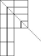
Figure 1: The (2,2,1,1) Young diagram

Before proving this theorem, we now consider an example $\lambda=\{2,2,1,1\}$ as shown in Fig. 1. The corresponding Schur state is

$$|\lambda\rangle=(-)\psi_{-3/2}\psi_{-7/2}^{*}\psi_{-1/2}\psi_{-1/2}^{*}|vac\rangle\,.$$

From the formalism of $H_{d}$, the energy eigenvalue is contributed by the following terms

$$\frac{2}{3}\left(\frac{3}{2}-1\right)\psi_{-3/2}\psi_{3/2}^{*}\,,\,\left((\frac{7}{2}-\frac{1}{2})(\frac{7}{2}+\frac{1}{6})\right)\psi_{-7/2}^{*}\psi_{7/2}$$

$$\frac{2}{3}\left\{\left(7+\frac{3}{2}\right)\psi_{-3/2}\psi_{-7/2}^{*}\psi_{7/2}\psi_{3/2}^{*}+\left(1+\frac{1}{2}\right)\psi_{-1/2}\psi_{-1/2}^{*}\psi_{1/2}\psi_{-1/2}^{*}\right.$$

$$\hskip 14.22636pt+\left(7+\frac{1}{2}\right)\psi_{-1/2}\psi_{-7/2}^{*}\psi_{7/2}\psi_{1/2}^{*}+\left(1+\frac{3}{2}\right)\psi_{-3/2}\psi_{-1/2}^{*}\psi_{1/2}\psi_{3/2}^{*}$$

$$\left.\hskip 14.22636pt+\left(1-\frac{3}{2}\right)\psi_{-3/2}\psi_{-1/2}\psi_{-1/2}^{*}\psi_{3/2}^{*}-\left(7-\frac{1}{2}\right)\psi_{-1/2}^{*}\psi_{-7/2}^{*}\psi_{7/2}\psi_{1/2}\right\}\,.$$

Combine all of them, we have the eigenvalue of $H_{d}$

$$E_{\lambda}^{d}=\frac{1}{3}+11+\frac{2}{3}(10+10-7)=20=16+4\,.$$

Proof of Theorem 2

For a generic Schur state, the proof of Theorem 2 is following. A generic Schur state is denoted by

$$|\lambda\rangle=(-)^{\sum_{i}^{d(\lambda)}\left(m_{i}-\frac{1}{2}\right)}\prod_{i}^{d(\lambda)}\psi_{-n_{i}}\psi_{-m_{i}}^{*}|vac\rangle\,.$$ (38)

Acting on it, the first two terms of $H_{d}$ contribute

$$\sum_{i}^{d(\lambda)}\frac{1}{3}(n_{i}-\frac{1}{2})+\left(m_{i}-\frac{1}{2}\right)\left(m_{i}+\frac{1}{6}\right)\,.$$ (39)

The third term contains

$$\left(\begin{array}[]{c}2d(\lambda)\\ 2\end{array}\right)=d(\lambda)(2d(\lambda)-1)$$

terms. We can have three independent picking strategies. Among them there are $d(\lambda)^{2}$ terms picked from a pair of $\psi$ and $\psi^{*}$ which we call $\psi\psi^{*}$-strategy. Other terms are from two fermionic modes picked from either the set of all $\psi$’s or $\psi^{*}$’s (the $\psi\psi$-strategy and $\psi^{*}\psi^{*}$-strategy).

We first consider the $\psi\psi^{*}$ -strategy. The contribution is

$$E_{\psi\psi^{*}}=\frac{2}{3}\sum_{i,j=1}^{d(\lambda)}(2m_{i}+n_{j})\,.$$ (40)

The $\psi\psi$ strategy has a signature contribution (-1). Its contribution to the total energy is

$$E_{\psi\psi}=\frac{2}{3}\sum_{i>j}^{d(\lambda)}(2n_{i}-n_{j})\,.$$ (41)

Similarly, the $\psi^{*}\psi^{*}$ -strategy gives rise to

$$E_{\psi^{*}\psi^{*}}=\frac{2}{3}\sum_{i<j}^{d(\lambda)}(-2m_{i}+m_{j})\,.$$ (42)

The summation conditions $i>j$ or $i<j$ reflects the condition $k+l>0$. Thus we have translated the Theorem 2 into the form that

$$\sum_{i}^{\ell(\lambda)}(\lambda_{i}^{t})^{2}=\sum_{i}^{d(\lambda)}\frac{1}{3}(n_{i}-\frac{1}{2})+\left(m_{i}-\frac{1}{2}\right)\left(m_{i}+\frac{1}{6}\right)$$ (43)

$$+\frac{2}{3}\left(\sum_{i,j=1}^{d(\lambda)}(2m_{i}+n_{j})+\sum_{i>j}^{d(\lambda)}(2n_{i}-n_{j})+\sum_{i<j}^{d(\lambda)}(-2m_{i}+m_{j})\right)\,.$$

We use mathematical induction to prove it here. A direct proof can be found in Appendix.

Suppose the relation holds for a Young diagram $\lambda$, with $|\lambda|=n$. We will prove it holds for adding one more box to $\lambda$ under or right to the certain position $(i,j)$. These two different cases are following.

Case I: $\lambda_{j}^{t}\geq j$ $\lambda^{t}_{j-1}>i$ and the box is attached just under the $(i,j)$ box, so that

$$m_{j}\rightarrow m_{j}+1\,.$$

The change of R.H.S of (43) will be

$$\Delta_{RHS} = \left(2m_{j}+\frac{2}{3}\right)+\frac{2}{3}\left(2d(\lambda)+j-1-2(d(\lambda)-j)\right)$$

$$= 2m_{j}+2j=2\lambda_{j}^{t}+1=\Delta_{LHS}\,.$$

Case II: $\lambda_{i}\geq i$ $\lambda_{i-1}>j$, the box is attached to the right of the box $(i,j)$, so that

$$n_{i}\rightarrow n_{i}+1\,.$$

The change of R.H.S of (43) will be

$$\Delta_{RHS} = \frac{1}{3}+\frac{2}{3}(3i-2)=2i-1\,.$$ (45)

Notice that the $j+1$-th column has $\lambda_{j+1}^{t}=i-1$, so the change of L.H.S of (43) is

$$\Delta_{L.H.S}=i^{2}-(i-1)^{2}=2i-1=\Delta_{R.H.S}\,.$$

Now we conclude that the identity (43) holds for any Young diagram and the Theorem 2 is proved. Q.E.D.

3.5.2 $H_{t}$ squeezes the state

As argued previously, the $H_{t}$ always squeezes the original Young diagram $\lambda$ for a given Schur state to some “thinner” $\lambda^{\prime}$’s. To be precise after its action

$$\lambda^{\prime}<\lambda\quad\hbox{meaning}\quad\sum_{i=1}^{j}\lambda_{i}^{\prime}<\sum_{i=1}^{j}\lambda_{i},\,\text{for }\,j=1,2,\cdots\,.$$ (46)

To see this triangular property in a more transparent form, we first reduce the summation area from $r+s<0,k+l>0$ to $k+l>0,k+s<0,k>r$ and $k<r$. The $k<r$ case can be obtained from re-labeling the index ($r\leftrightarrow k$) and exchanging $\psi_{r}$ and $\psi_{k}$

$$\frac{1}{1-b^{2}}H_{t} = \sum_{\begin{subarray}{c}k+l>0,r+s+k+l=0\\ s,k,l\in\mathbb{Z}+\frac{1}{2}\end{subarray}}\left(\frac{2}{3}(2k-r)\right):\psi_{r}\psi_{s}^{*}\psi_{k}\psi_{l}^{*}:$$ (47)

$$= \sum_{\begin{subarray}{c}k+l>0,k+s<0\\ k>r,r+s+k+l=0\end{subarray}}\left(\frac{2}{3}(2k-r-2r+k)\right):\psi_{r}\psi_{s}^{*}\psi_{k}\psi_{l}^{*}:$$ (48)

$$= \sum_{\begin{subarray}{c}k+l>0,k+s<0\\ k>r,r+s+k+l=0\end{subarray}}2(k-r):\psi_{r}\psi_{s}^{*}\psi_{k}\psi_{l}^{*}:\,.$$ (49)

$H_{t}$ is simplified and the summation area is decomposed into five cases

$$\frac{1}{1-b^{2}}H_{t} = 2\sum_{\begin{subarray}{c}k+l>0,k+s<0\\ k>r,k+l+r+s=0\end{subarray}}(k-r):\psi_{r}\psi_{s}^{*}\psi_{k}\psi_{l}^{*}:$$

$$= 2\sum_{n=1,k>r>0}^{n=s-1/2}(k-r)\psi_{-k-n}^{*}\psi_{-r+n}^{*}\psi_{r}\psi_{k}$$

$$+2\sum_{n=1,k>r>0}^{n=[(k-r-1)/2]}(r-k+2n)\psi_{-k+n}\psi_{-r-n}\psi_{r}^{*}\psi_{k}^{*}$$

$$+2\sum_{n=1,k,r>0}^{n=r-1/2}(k+r-n)\psi_{-r+n}\psi_{-k-n}^{*}\psi_{k}\psi_{r}^{*}$$

$$+2\sum_{k>r>0,s>0}(r-k)\psi_{-r-s-k}^{*}\psi_{r}\psi_{k}\psi_{s}^{*}$$

$$+2\sum_{k>r>0,s>0}(k-r)\psi_{-k}\psi_{-s}^{*}\psi_{-r}\psi_{r+s+k}^{*}\,.$$

Acting on a Schur state corresponding to a Young diagram $H_{t}$ gives rise to the following five processes.

Case I:The first line of the second equality in (3.5.2) annihilates two columns of the corresponding Young diagram of length $r$ and $k$ (k>r) and creates two new columns of length $k+n$ and $r-n$, which makes long column longer and short column shorter simultaneously. So it squeezes the Young diagram.

Case II: The second line annihilates two rows of length $r$ and $k$ (k>r) and generates two new rows of length $k-n$ and $r+n$, which makes long row shorter and short row longer, but not longer than the new shorter row, also, it squeezes the Young diagram.

Case III: The third line annihilates one row of length $k$ and one column $r$ and generates a shorter row (length $r-n$) and a longer column (length $k+n$).

Case IV: The fourth line annihilates two column of length $r$ and $k$ (k>r) and one row of length $s$ and generates a single column of length $r+k+s$ .

Case V: The fifth line annihilates a long row of length $r+k+s$ into three short columns of lengths $r$, $k$, $s$ respectively .

From the above analysis, we conclude that the $H_{t}$, when acting on a Schur state, will generate series of squeezed states. We call this property the fermionic triangularization.

3.6 Integrability

The triangular property means the eigenstate can be understood as $|P_{\lambda}(\psi\psi^{*})\rangle$, with

$$P_{\lambda}=s_{\lambda}+\sum_{\mu<\lambda}c_{\lambda,\mu}s_{\mu}\,.$$

This ansatz is due to the eigenstate of bosonic $H$ is a function of bosonic oscillators $a_{-n}$’s. When $a_{-n}$ acts on a coherent basis, the eigenstate will be a power sum symmetric function

$$\tilde{a}_{-n}\exp\left(\sum_{i,n}b\frac{a_{n}}{-n}z_{i}^{n}\right)|0\rangle=\exp\left(\sum_{i,n}b\frac{a_{n}}{-n}z_{i}^{n}\right)\sum_{i}z_{i}^{n}|0\rangle$$

$$\Rightarrow\tilde{a}_{-n}\simeq\sum_{i}z_{i}^{n}=p_{n}(z_{i})\,.$$ (52)

It in turn determines the eigenstate itself as a symmetric function. The eigenvalue of $H$ is

$$H|P_{\lambda}(\psi\psi^{*})\rangle=E_{\lambda}^{\beta}|P_{\lambda}(\psi\psi^{*})\rangle\,.$$ (53)

Let us consider the leading Schur function $s_{\lambda}$. Because $H_{t}$ changes basis, the eigenvalue should come from the action of $H_{0}^{\beta}$ on

$$|s_{\lambda}\rangle=s_{\lambda}(\psi\psi^{*})|vac\rangle\,.$$

The equation (53), has an explicit solution (up to a constant similarity transformation) that

$$|P_{\lambda}\rangle\propto R(E)|s_{\lambda}\rangle\,,$$

where

$$R(E)=\frac{1}{1-\frac{1-b^{2}}{E_{\lambda}^{\beta}-H_{0}^{\beta}}H_{t}}\,.$$ (54)

This solution can be derived as follows. We first rewrite $H$ as

$$H=E-(E-H_{0}^{\beta})\left(1-\frac{1-b^{2}}{E-H_{0}^{\beta}}H_{t}\right)\,$$ (55)

then

$$H|P_{\lambda}\rangle = \left(E_{\lambda}^{\beta}-(E_{\lambda}^{\beta}-H_{0}^{\beta})\left(1-\frac{1-b^{2}}{E_{\lambda}^{\beta}-H_{0}^{\beta}}H_{t}\right)\right)R(E)|s_{\lambda}\rangle$$

$$= E_{\lambda}^{\beta}R(E)|s_{\lambda}\rangle-(E_{\lambda}^{\beta}-H_{0}^{\beta})|s_{\lambda}\rangle=E_{\lambda}^{\beta}|P_{\lambda}\rangle\,.$$

Notice that till now we have used the deformed bosonic oscillators $\tilde{a}$. It is not convenient when we consider the standard symmetric function formulae. We need to introduce a similarity transformation that transforms $\tilde{a}$’s back to $a$’s.

$$D=\exp\bigl{(}-\log(b)(\tilde{q}\tilde{a}_{0}+\sum_{n>0}\tilde{a}_{-n}\tilde{a}_{n}/n)\bigr{)}\,,$$ (57)

or equivalently, we have a fermionic formalism

$$D_{\pm}=b^{\pm\frac{1}{2}\sum_{r>0}(\psi_{-r}\psi_{r}^{*}+\psi_{-r}^{*}\psi_{r})}\,,$$ (58)

where $\pm$ means acting on bra(left) or ket(right) state respectively.

4 Laughlin state and its Hamiltonian

The Laughlin state is defined as

$$\Psi_{L}(\{z_{i}\})=\prod_{i<j}(z_{i}-z_{j})^{b^{2}}\exp\left(-\sum_{i}\frac{|z_{i}^{2}|}{4\ell}\right)\,,$$ (59)

where $b^{-2}=\nu\in\mathbb{Z}$ is the filling fraction. In the formula

$$\ell=\sqrt{\frac{\hbar}{eB}}$$

is the basic magnetic length scale. Usually it is normalized to be 1. $e$ stands for the electron charge and $B$ is the external magnetic field strength. The Gaussian factor

$$\exp\left(-\sum_{i}\frac{|z_{i}^{2}|}{4\ell}\right)\,,$$

will be ignored later on since it will bring in excessive clutters.

The Laughlin wavefunction can be understood as follows. Consider there are $N$ quasi-particles containing in the interior of a disk of area $A_{N}=2N\pi b^{2}$. The ground state of this system is a correlation function of these $N$ free quasi-particles in a background magnetic field, which in general makes the total charge to be zero, that is, a neutral correlation function. We define the vertex operator for a quasi-particle

$$V_{b}(z)=e^{b\phi(z)}\,.\,$$

The density $\rho_{0}$ of the $\phi$ field on the disk, for a ground state, should be uniform anywhere. Otherwise a density wave will be excited. It is simply

$$\rho_{0} = \frac{N}{2\pi Nb^{2}}=\frac{1}{2\pi b^{2}}\,.$$

Thus the background charge is

$$S=e^{-b\int d^{2}w\rho_{0}\phi(w)}\,.$$

Without this factor, the correlation function will vanish. Now the correlation function is written as

$$\langle 0\prod_{i=1}^{N}V_{b}(z_{i})S|0\rangle = \Bigg{\langle}\prod_{i=1}^{N}e^{b\phi(z)}\exp\bigg{(}-b\int d^{2}w\rho_{0}\phi(w)\bigg{)}\Bigg{\rangle}$$ (60)

$$= \prod_{i<j}^{N}(z_{i}-z_{j})^{b^{2}}\equiv\tilde{\Psi}_{L}(\{z_{i}\})$$

Here we have defined the so-called "reduced wave function" $\tilde{\Psi}_{L}(\{z_{i}\})$ without the Gaussian factor. We now can consider the polynomial excitations of this ground state and moreover the behind integrability of this system.

4.1 From ground state to the Hamiltonian

As we have done in the case of Calogero-Sutherland model, we now propose a Hamiltonian exactly has this Laughlin state as its ground state, that is,

$$H_{L} = \sum_{i}(\partial_{i}+\partial_{i}(\ln\tilde{\Psi}\{z_{i}\}))(\partial_{i}-\partial_{i}(\ln\tilde{\Psi}\{z_{i}\})).$$ (61)

Here $\partial_{i}=\partial/\partial x_{i}\equiv z_{i}\partial_{z_{i}}$, or equivalently, $z_{i}=e^{x_{i}}$. By separating out the ground state contribution as follows, we have

$$\tilde{{H}} = \tilde{(\Psi}\{z_{i}\})^{-1}H_{L}\tilde{\Psi}\{z_{i}\}$$

$$= \sum_{i}\left(z_{i}\partial_{z_{i}}+2z_{i}\partial_{z_{i}}(\ln\tilde{\Psi}\{z_{i}\})z_{i}\partial_{z_{i}}\right)$$

$$= \sum_{i}(z_{i}\partial_{z_{i}})^{2}-2b^{2}\sum_{i<j}\frac{z_{i}^{2}\partial_{z_{i}}}{z_{i}-z_{j}}$$

$$= \sum_{i}(z_{i}\partial_{z_{i}})^{2}-b^{2}\sum_{i<j}\frac{z_{i}^{2}\partial_{z_{i}}-z_{j}^{2}\partial_{z_{j}}}{z_{i}-z_{j}}\,.$$

When acting on the normal ordered vertex operators, we have

$$z_{i}\partial_{z_{i}}\prod_{j}^{N}\exp\left(b\sum_{n,j}\frac{a_{-n}}{n}z_{j}^{n}\right)|0\rangle = b\sum_{n}a_{-n}z_{i}^{n}\prod_{j}^{N}\exp\left(b\sum_{n,j}\frac{a_{-n}}{n}z_{j}^{n}\right)|0\rangle\,,$$

$$(z_{i}\partial_{z_{i}})^{2}\prod_{j}^{N}\exp\left(b\sum_{n,j}\frac{a_{-n}}{n}z_{j}^{n}\right)|0\rangle = b^{2}\sum_{n,m}a_{-n}a_{-m}z_{i}^{n+m}\prod_{j}^{N}\exp\left(b\sum_{n,j}\frac{a_{-n}}{n}z_{j}^{n}\right)|0\rangle$$

$$+ b\sum_{n}na_{-n}z_{i}^{n}\prod_{j}^{N}\exp\left(b\sum_{n,j}\frac{a_{-n}}{n}z_{j}^{n}\right)|0\rangle\,,$$

$$a_{k}\prod_{j}^{N}\exp\left(b\sum_{n,j}\frac{a_{-n}}{n}z_{j}^{n}\right)|0\rangle = \sum_{i}bz_{i}^{n}\prod_{j}^{N}\exp\left(b\sum_{n,j}\frac{a_{-n}}{n}z_{j}^{n}\right)|0\rangle\,,$$ (63)

$$\frac{z_{i}^{2}\partial_{z_{i}}-z_{j}^{2}\partial_{z_{j}}}{z_{i}-z_{j}}\prod_{j}^{N}\exp\left(b\sum_{n,j}\frac{a_{-n}}{n}z_{j}^{n}\right)|0\rangle$$

$$=\frac{b\sum_{n}a_{-n}\left(z_{i}^{n+1}-z_{j}^{n+1}\right)}{z_{i}-z_{j}} \prod_{j}^{N}\exp\left(b\sum_{n,j}\frac{a_{-n}}{n}z_{j}^{n}\right)|0\rangle$$

$$=b\sum_{n}a_{-n}(z_{i}^{n}+z_{i}^{n-1}z_{j}+ \cdots +z_{i}z_{j}^{n-1}+z_{j}^{n})\prod_{j}^{N}\exp\left(b\sum_{n,j}\frac{a_{-n}}{n}z_{j}^{n}\right)|0\rangle\,,$$ (64)

and substituting (63) into (4.1), we have the free part of (4.1) as

$$\tilde{{H}_{0}}=\sum_{n>0}na_{-n}a_{n}+b\sum_{n,m>0}a_{-n}a_{-m}a_{n+m}$$

We need to be careful with the interaction term (64). The summation on $i,\,j$ is not arbitrary. To turn this term into bosonic operator formalism, we have to do a trick as follow. Firstly, we change the summation from $i<j$ to $i\neq j$. It gives rise to a simple $\frac{1}{2}$ factor. Secondly, we add $i=j$ terms into the summation and then finally subtract these terms. Follow these steps, we have

$$b^{3}\sum_{i<j}\,\sum_{n>0}a_{-n}(z_{i}^{n}+z_{i}^{n-1}z_{j}+ \cdots +z_{i}z_{j}^{n-1}+z_{j}^{n})=\frac{b}{2}\sum_{n,m>0}a_{-n-m}a_{n}a_{m}$$

$$-\frac{1}{2}b^{2}\sum_{n>0}na_{-n}a_{n} + b^{2}(N-1)\sum_{n>0}a_{-n}a_{n\,,}$$ (65)

The last term of (65) is an irrelevant total energy of free quasi-particles. When acting on a level $n$ state, it gives rise to an eigen-energy

$$E_{ir}|n\rangle=b^{2}(N-1)n|n\rangle\,$$

as expected which describes a system of $N-1$ copies of non-interacting bosonic oscillators with the frequency $b^{2}$. Therefore we ignore its contribution and now we obtain the operator formalism of $H_{L}$

$$H_{L}=\sum_{n}\left(1-\frac{b^{2}}{2}\right)na_{-n}a_{n}+\sum_{n,m}b\left(a_{-n}a_{-m}a_{n+m}+\frac{1}{2}a_{-n-m}a_{n}a_{m}\right)\,.$$ (66)

4.2 Fermionization of $H_{L}$

Define the deformed bosonic modes as

$$2b^{-1}\tilde{a}_{n} = a_{n}\,,\quad\frac{1}{2}b\tilde{a}_{-n}=a_{-n\,,}$$ (67)

so that the triple-$a$ terms in (66) now becomes

$$\sum_{n,m>0}\left(\frac{1}{2}b^{2}\tilde{a}_{-n}\tilde{a}_{-m}\tilde{a}_{n+m}+\tilde{a}_{-n-m}\tilde{a}_{n}\tilde{a}_{m}\right)$$

$$= \sum_{n,m>0}\left(\tilde{a}_{-n}\tilde{a}_{-m}\tilde{a}_{n+m}+\tilde{a}_{-n-m}\tilde{a}_{n}\tilde{a}_{m}\right)-(1-\frac{b^{2}}{2})\tilde{a}_{-n}\tilde{a}_{-m}\tilde{a}_{n+m}\,.$$

It is straightforward to write down the fermionic formalism as the case of the Calogero-Sutherland model in previous section. Hence we get

$$H_{L}=H_{0}+(1-\frac{b^{2}}{2})H_{d}+(1-\frac{b^{2}}{2})H_{t}\equiv H_{l}+(1-\frac{b^{2}}{2})H_{t}\,.$$ (68)

The eigen-energy for this Hamiltonian is

$$E_{\lambda}^{Lau}=\sum_{i=1}^{\lambda_{1}^{t}}(\lambda_{i})^{2}-\frac{b^{2}}{2}\sum_{i=1}^{\lambda_{1}}(\lambda_{i}^{t})^{2}\,.$$ (69)

The corresponding excitation state is

$$|P_{\lambda}^{Lau}\rangle=D^{Lau}\frac{1}{1-\frac{1-b^{2}/2}{E_{\lambda}^{Lau}-H_{l}}H_{t}}s_{\lambda}(\psi\psi^{*})|vac\rangle\,,$$

where $D^{Lau}$ is the similarity transformation related to (67).

$$D^{Lau}=\exp\bigl{(}-\log(b/2)(\tilde{q}\tilde{a}_{0}+\sum_{n>0}\tilde{a}_{-n}\tilde{a}_{n}/n)\bigr{)}\,,$$ (70)

and the fermionic expression:

$$D_{\pm}^{Lau}=\left(\frac{b}{2}\right)^{\pm\sum_{r>0}(\psi_{-r}\psi_{r}^{*}+\psi_{-r}^{*}\psi_{r})}\,.$$ (71)

Notice that the polynomial is not a new polynomial, it is a Jack polynomial with the parameter $\beta=\frac{b^{2}}{2}\,.$

Since the integrability of the Laughlin theory is exactly the same as that of CS model we ignore its analysis here.

5 Halperin State and Two-layer System

Now we can consider the two-layer system. The corresponding ground state wavefunction is the Halperin state, which reads

$$\tilde{\Psi}_{H}\left({z_{i}},{w_{j}}\right)=\prod_{i<j}^{N}(z_{i}-z_{j})^{p}\prod_{m<n}^{M}(w_{m}-w_{n})^{q}\prod_{i,m}^{N,M}(z_{i}-w_{m})^{r}\,.$$ (72)

The complexity of this wave-function lies in that it involves an interaction between two layers. Let us first define the bosonic fields

$$\phi^{1}(z) = q_{0}^{1}+a_{0}^{1}\ln z+\sum_{n\neq 0}\frac{a_{-n}^{1}}{n}z^{n}\,,$$

$$\phi^{2}(w) = q_{0}^{2}+a_{0}^{2}\ln w+\sum_{n\neq 0}\frac{a_{-n}^{2}}{n}w^{n}\,,$$

with commutation relation

$$[a_{n}^{I}\,,\,a_{m}^{J}]=n\delta^{IJ}\delta_{n+m,0}\,,\,n,m\in\mathbb{Z},\,I,J\in{1,2}\,.$$

The related coordinate system is defined as

$$Z_{I} = z_{I},\,\mbox{if}\,\ I\leq N\,,$$

$$Z_{I} = w_{I-N}\,,\,if\ \,N<I\leq N+M\,,$$

$$\partial_{I} = Z_{I}\partial_{Z_{I}}\,,$$

we can now write down the Hamiltonian of this system as

$$H^{Hal} = \sum_{I}(\partial_{I}-2\partial_{I}(\ln\tilde{\Psi}_{H}(Z_{I}))\partial_{I}$$

$$= \sum_{i=1}^{N}\left(z_{i}\partial_{z_{i}}-2z_{i}\partial_{z_{i}}\left(\ln\prod_{i<j}(z_{i}-z_{j})^{p}\right)\right.$$

$$+\left.2z_{i}\partial_{z_{i}}\left(\ln\prod_{i,m}(z_{i}-w_{m})^{r}\right)\right)z_{i}\partial_{z_{i}}$$

$$+ \sum_{m=1}^{M}\left(w_{m}\partial_{w_{m}}-2w_{m}\partial_{w_{m}}\left(\ln\prod_{m<n}(w_{m}-w_{n})^{q}\right)\right.$$

$$+\left.2w_{m}\partial_{w_{m}}\left(\ln\prod_{i,m}(z_{i}-w_{m})^{r}\right)\right)w_{m}\partial_{w_{m}}$$

$$= H_{L}(p)+H_{L}(q)+2r\sum_{m,i}\frac{z_{i}^{2}\partial_{z_{i}}}{z_{i}-w_{m}}-2r\sum_{m,i}\frac{w_{m}^{2}\partial_{w_{m}}}{z_{i}-w_{m}}\,,$$

$$= H_{L}(p)+H_{L}(q)+2r\sum_{n\geq 0,m,i}\left(\frac{w_{m}}{z_{i}}\right)^{n}z_{i}\partial_{z_{i}}-2r\sum_{n>0,m,i}\left(\frac{w_{m}}{z_{i}}\right)^{n}w_{m}\partial_{w_{m}}\,\,,$$

where $H_{L}(p)$ is the Laughlin Hamiltonian defined before in which $b^{2}\rightarrow p\,.$ The vertex operators in this system are

$$V_{\sqrt{p}}^{1}(z)=e^{\sqrt{p}\phi^{1}(z)}\,,\>V_{\sqrt{q}}^{2}(w)=e^{\sqrt{q}\phi^{2}(w)}\,.$$

The differential operators relate to operators and power-sum polynomials are defined as follows

$$z_{i}\partial_{z_{i}}\prod_{i=1}^{N}V_{\sqrt{p}}^{1,-}(z_{i}) = \sum_{n>0}\sqrt{p}a_{-n}^{1}z_{i}^{n}\prod_{i=1}^{N}V_{\sqrt{p}}^{1,-}(z_{i})\,,$$

$$w_{m}\partial_{w_{m}}\prod_{j=1}^{M}V_{\sqrt{q}}^{2,-}(w_{j}) = \sum_{n>0}\sqrt{q}a_{-n}^{2}w_{j}^{n}\prod_{n=1}^{M}V_{\sqrt{q}}^{2,-}(w_{j})\,,$$

$$a_{n}^{1}\prod_{i=1}^{N}V_{\sqrt{p}}^{1,-}(z_{i})|0\rangle = \sqrt{p}\sum_{i}z_{i}^{n}\prod_{i=1}^{N}V_{\sqrt{p}}^{1,-}(z_{i})|0\rangle$$

$$a_{n}^{2}\prod_{j=1}^{N}V_{\sqrt{p}}^{2,-}(w_{j})|0\rangle = \sqrt{q}\sum_{i}w_{j}^{n}\prod_{i=1}^{N}V_{\sqrt{p}}^{1,-}(w_{j})|0\rangle$$

Therefore we have

$$2r\sum_{n\geq 0,m,i}\left(\frac{w_{m}}{z_{i}}\right)^{n}z_{i}\partial_{z_{i}} \rightarrow 2r\frac{1}{\sqrt{q}}\sum_{\begin{array}[t]{c}n\geq 0\\ m>0\end{array}}a_{-n}^{1}a_{n-m}^{1}a_{m}^{2}\,,$$

$$2r\sum_{n>0,m,i}\left(\frac{w_{m}}{z_{i}}\right)^{n}w_{m}\partial_{w_{m}} \rightarrow 2r\frac{1}{\sqrt{p}}\sum_{\begin{array}[t]{c}n>0\\ m>0\end{array}}a_{-m}^{1}a_{-n}^{2}a_{n+m}^{2}\,.$$

It is now easy to write down the bosonic operator formalism, we have

$$H^{Hal} = H_{L}(p,a^{1})+H_{L}(q,a^{2})+H_{int}\,,$$

$$H_{int} = 2r\left(\frac{1}{\sqrt{q}}\sum_{\begin{array}[t]{c}n\geq 0\\ m>0\end{array}}a_{-n}^{1}a_{n-m}^{1}a_{m}^{2}-\frac{1}{\sqrt{p}}\sum_{\begin{array}[t]{c}n>0\\ m>0\end{array}}a_{-m}^{1}a_{-n}^{2}a_{n+m}^{2}\right)$$

$$= r\left(\frac{1}{\sqrt{q}}\sum_{m>0}L_{-m}^{1}a_{m}^{2}+\sum_{n,m>0}(\frac{1}{\sqrt{q}}a_{-n}^{1}-\frac{2}{\sqrt{p}}a_{-n}^{2})a_{-m}^{1}a_{n+m}^{2}\right)\,.$$

Notice that the $H_{int}$ is a fascinating interaction. It is always a triangular term such that it subtracts boxes in Young diagram $\mu$ on layer-2 and adds the same number of boxes into Young diagram $\lambda$ on layer-1. The Hilbert space of this Hamiltonian is expanded by coupled bi-Jack functions, that is,

$$|\Omega_{\lambda,\mu}^{0}\rangle=|P_{\lambda}^{1}(p/2)\rangle\otimes|P_{\mu}^{2}(q/2)\rangle\,.$$

It is not an eigenstate of the Halperin Hamiltonian, but only a highest weight state of the eigenstate, which can be obtained as following formula

$$|\Omega_{\lambda,\mu}^{r}\rangle=\frac{1}{1-\frac{1}{E_{\lambda,\mu}-H_{L}(p)-H_{L}(q)}H_{int}}|\Omega_{\lambda,\mu}^{0}\rangle\,,$$

where the eigen-energy is written as

$$E_{\lambda,\mu}=\sum_{i}^{\lambda_{1}^{t}}(\lambda_{i})^{2}+\sum_{j}^{\mu_{1}^{t}}(\mu_{j})^{2}-\frac{p}{2}\sum_{k}^{\lambda_{1}}(\lambda_{k}^{t})^{2}-\frac{q}{2}\sum_{l}^{\mu_{1}}(\mu_{k}^{t})^{2}\,.$$

The fermionization of the Hamiltonian as in (72) is not hard. Let us first consider the first term in $H_{int}$ . It is

$$H_{int}^{1} = \frac{2r}{\sqrt{q}}\sum_{\begin{array}[t]{c}n\geq 0\\ m>0\end{array}}a_{-n}^{1}a_{n-m}^{1}a_{m}^{2}$$

$$= \frac{2r}{\sqrt{q}}\left(\sum_{\begin{array}[t]{c}r,s,k,l,u\in\mathbb{Z}+\frac{1}{2}\\ r+s+k+l=-m<0\end{array}}:\psi_{r}^{1}\psi_{s}^{1*}\psi_{k}^{1}\psi_{l}^{1*}\psi_{-u}^{2}\psi_{m+u}^{2*}:\right.$$

$$\hskip 10.00002pt\hskip 10.00002pt+\left.\sum_{u\in\mathbb{Z}+\frac{1}{2},m>0}:\psi_{-u}^{2}\psi_{m+u}^{2*}:(\text{Contractions})\right)\,,$$

where the contractions is calculated as

Contractions $$= \sum_{\begin{array}[t]{c}\begin{array}[t]{c}n,r>0\end{array}\end{array}}:(\psi_{-r}^{1}\psi_{-n+r}^{1*}-\psi_{-r-n}^{1*}\psi_{r}^{1})(\psi_{-s}^{1}\psi_{n-m+s}^{1*}-\psi_{n-m-s}^{1*}\psi_{s}^{1}):\,,$$

$$= \sum_{r>0}(\psi_{-r}^{1}\psi_{r-m}^{1*}+\psi_{-m-s}^{1*}\psi_{s}^{1})\,.$$

Therefore

$$H_{int}^{1} = \frac{2r}{\sqrt{q}}\left(\sum_{\begin{array}[t]{c}r,s,k,l,u\in\mathbb{Z}+\frac{1}{2}\\ r+s+k+l=-m<0\end{array}}:\psi_{r}^{1}\psi_{s}^{1*}\psi_{k}^{1}\psi_{l}^{1*}\psi_{-u}^{2}\psi_{m+u}^{2*}:\right.$$

$$\hskip 10.00002pt\hskip 10.00002pt+\left.\sum_{\begin{array}[t]{c}u>0\\ r,m>0\end{array}}(\psi_{-u}^{2}\psi_{m+u}^{2*}-\psi_{m-u}^{2*}\psi_{u}^{2})(\psi_{-r}^{1}\psi_{r-m}^{1*}+\psi_{-m-r}^{1*}\psi_{r}^{1})\right)\,.$$

Similarly, we have

$$H_{int}^{2} = -\frac{2r}{\sqrt{p}}\sum_{\begin{array}[t]{c}n,m>0\end{array}}a_{-m}^{1}a_{-n}^{2}a_{n+m}^{2}$$

$$= -\frac{2r}{\sqrt{p}}\left(\sum_{\begin{array}[t]{c}r,s,k,l,u\in\mathbb{Z}+\frac{1}{2}\\ r+s+k+l=m>0\end{array}}:\psi_{r}^{2}\psi_{s}^{2*}\psi_{k}^{2}\psi_{l}^{2*}\psi_{-u}^{1}\psi_{-m+u}^{1*}:\right.$$

$$\hskip 10.00002pt\hskip 10.00002pt+\left.\sum_{u\in\mathbb{Z}+\frac{1}{2},m>0}:\psi_{-u}^{1}\psi_{-m+u}^{1*}:(\text{Contractions})\right)$$

$$=-\frac{2r}{\sqrt{p}}\left(\sum_{\begin{array}[t]{c}r,s,k,l,u\in\mathbb{Z}+\frac{1}{2}\\ r+s+k+l=m>0\end{array}}:\psi_{r}^{2}\psi_{s}^{2*}\psi_{k}^{2}\psi_{l}^{2*}\psi_{-u}^{1}\psi_{-m+u}^{1*}:\right.$$

$$\hskip 10.00002pt\hskip 10.00002pt+\left.\sum_{\begin{array}[t]{c}u,m>0\\ r>0\end{array}}(\psi_{-u}^{1}\psi_{-m+u}^{1*}-\psi_{-m-u}^{1*}\psi_{u}^{1})(\psi_{-r}^{2}\psi_{r+m}^{2*}+\psi_{m-r}^{2*}\psi_{r}^{2})\right)\,.$$

Though this fermionic formalism is not effective in calculating the eigenstate, it plays an important role in deriving the behind tau-function and its Hirota integrability of this system. Actually, the fermionic formalism completely defines the fermionic orbit of a generator of $GL(\infty)$ which in turn determine the tau-function of this theory. We are working in detail in this direction.

5.1 Similarity transformation

As explained before, we need to do a similarity transformation to recover the deformed operator formalism of eigenstates to a standard operator formalism. It is easy to write down this similarity transformation, that is

$$D^{Hal}=D^{Lau}(b^{2}\rightarrow p,\,a\rightarrow a^{1})D^{Lau}(b^{2}\rightarrow q,\,a\rightarrow a^{2})\,.$$

6 Conclusions and Future Works

In conclusion, we introduce a systematic way to extract the integrability of several models. For CS model, we express the Hamiltonian in bosonic as well as fermionic representations. The eigenstate and eigenvalue are obtained explicitly. The construction of Jack state, in the fermionic representation, is highly involved in the fermionic triangularization of fermionic Hamiltonian of the CS model. For Laughlin and Halperin states, which can be seen as solitonic wavefunction, we construct the corresponding Hamiltonians in the same manner as CS model. We obtain their bosonic and fermionic representations. The explicit solutions, e.g. excitations and eigenvalues, are exactly solved. The integrability of Laughlin state, is the same as that of CS model, while for Halperin state, the integrability is determined also by the triangularization nature of the Hamiltonian.

There are several problems worthy of exploring in the future. Firstly, though the integrability in this article are inherited from free fermions, it is not clear to the authors that how to construct the integrable hierarchies. In soliton theory, the integrable hierarchy can be determined by the Lax operators. The Lax method is not the expected one for solving the problem since there are in general integration operators (the pseudo-differential operators) additional to usual differential operators. A possible solution may be the inverse scattering method, which will relate the integrable hierarchy to the inverse scattering equation[7]. This hierarchy tells us how integral of motions can be constructed by a recursive relation. A higher level integral of motion determines a refiner excitation structure of the model[18]. Secondly, for FQHEs, people believe special Jack polynomial may be related to certain FQHE wavefunction. It still remains mysterious to us what kind of constraint leads to a truncation of the fusion rule of Jack polynomials. Thirdly, we expect a direct generalization of our analysis to Haldane-Shastry model[15, 26, 27], or the spin CS model, we are working on that.

Appendix

We will denote a partition by its parts $(\lambda_{1},\lambda_{2},\cdots,\lambda_{\lambda^{t}_{1}})$ and the Frobenius notation $(\alpha_{1},\cdots,\alpha_{d}|\beta_{1},\cdots,\beta_{d})$ as well where $d$ is the diagonal length of $\lambda$. With this notation $n_{i}$ and $m_{i}$ in theorem 4 are related with $\alpha_{i}$ and $\beta_{i}$ in such a way that $n_{i}=\alpha_{i}+1/2$ and $m_{i}=\beta_{i}+1/2$. Theorem 4 is then written as

$$\sum_{i=1}^{\lambda_{1}}(\lambda^{t}_{i})^{2} = \sum_{i=1}^{d}\left[\frac{\alpha_{i}}{3}+\beta_{i}^{2}+\frac{2\beta_{i}}{3}\right]$$

$$\quad+\frac{2}{3}d\left[\sum_{i=1}^{d}(\alpha_{i}+2\beta_{i}+\frac{3}{2})+\sum_{i=1}^{d}2\alpha_{i}(i-1)\right.$$

$$\left.-\sum_{i=1}^{d}(d-i)\alpha_{i}+\sum_{i=1}^{d}\beta_{i}(i-1)-2\sum_{i=1}^{d}\beta_{i}(d-i)\right]$$

$$= \sum_{i=1}^{d}(\beta_{i}^{2}+2i\beta_{i}+2i\alpha_{i}-\alpha_{i})+d^{2}.$$

To prove this theorem we need two preliminary steps.

Step 1:

$$2[n(\lambda^{t})-n(\lambda)]=\sum_{i=1}^{d}\alpha_{i}(\alpha_{i}+1)-\beta_{i}(\beta_{i}+1).$$ (86)

It is obvious to prove the first step by using two very useful identities among several multi-number sets, namely

$$\{\beta_{i},(i\leq d)\}=\{0,1,\cdots,\lambda_{1}^{t}-1\}-\{i-\lambda_{i}-1,(d+1\leq i\leq\lambda_{1}^{t})\},$$

and similarly

$$\{\alpha_{i},(i\leq d)\}=\{0,1,\cdots,\lambda_{1}-1\}-\{i-\lambda^{t}_{i}-1,(d+1\leq i\leq\lambda_{1})\}.$$

These two identities are also very useful in proving step 2. Now let us compute

$$2[n(\lambda^{t})-n(\lambda)] = \sum_{i=1}^{\lambda_{1}^{t}}\lambda_{i}(\lambda_{i}-2i+1)$$

$$= \sum_{i=1}^{\lambda_{1}^{t}}(\lambda_{i}-i)^{2}+|\lambda|-\sum_{i=1}^{\lambda_{1}^{t}}i^{2}$$

$$= \sum_{i=1}^{d}\alpha_{i}^{2}+\sum_{i=d+1}^{\lambda_{1}^{t}}(-\lambda_{i}+i-1+1)^{2}+|\lambda|-\sum_{i=1}^{\lambda_{1}^{t}}i^{2}.$$

We apply one of the two identities. Therefore one term becomes

$$\sum_{i=d+1}^{\lambda_{1}^{t}}(-\lambda_{i}+i-1+1)^{2}=\sum_{i=0}^{\lambda^{t}_{1}-1}(i+1)^{2}-\sum_{i=1}^{d}(\beta_{i}+1)^{2}$$

and since

$$|\lambda|=\sum_{i=1}^{d}(\alpha_{i}+\beta_{i}+1),$$

combining all terms together we obtain the result in (86).

Step 2:

$$2[n(\lambda^{t})+n(\lambda)]=\sum_{i=1}^{d}(\alpha_{i}^{2}+\beta_{i}^{2}+4i\alpha_{i}+4i\beta_{i}-3\alpha_{i}-3\beta_{i})+2d(d-1).$$ (87)

To prove (87), we recall a formula in Macdonald’s book [20]

$$\sum_{x\in\lambda}h(x)=\sum_{(i,j)\in\lambda}(\lambda_{i}-i+\lambda^{t}_{j}-j+1)=n(\lambda^{t})+n(\lambda)+|\lambda|.$$

Hence

$$2[n(\lambda^{t})+n(\lambda)]=2\sum_{(i,j)\in\lambda}(\lambda_{i}-i+\lambda^{t}_{j}-j).$$

Now let us compute

$$\sum_{(i,j)\in\lambda}\lambda_{i}-i+\lambda_{j}^{t}-j = \sum_{i=1}^{\lambda^{t}_{1}}\sum_{j=1}^{\lambda_{i}}\lambda_{i}-i+\lambda_{j}^{t}-j$$

$$= \left[\sum_{i=1}^{d}\sum_{j=1}^{d}+\sum_{i=1}^{d}\sum_{j=d+1}^{\lambda_{i}}+\sum_{j=1}^{d}\sum_{i=d+1}^{\lambda^{t}_{j}}\right](\lambda_{i}-i+\lambda_{j}^{t}-j).$$

The regions of the summation are shown in Fig. 2.

Figure 2: The three regions of a Young diagram are separated by solid lines, thick lines, and dashed lines.

The square region surrounded by solid lines is simply

$$\sum_{i=1}^{d}\sum_{j=1}^{d}(\lambda_{i}-i+\lambda_{j}^{t}-j)=d\sum_{i=1}^{d}(\alpha_{i}+\beta_{i}).$$

Now let us compute the sum for the region surrounded by the thick lines.

$$\sum_{i=1}^{d}\sum_{j=d+1}^{\lambda_{i}}(\lambda_{i}-i)=\sum_{i=1}^{d}(\lambda_{i}-i)(\lambda_{i}-d)=\sum_{i=1}^{d}(\lambda_{i}^{2}-i\lambda_{i}-d\lambda_{i}+id).$$

We obtain

$$\sum_{i=1}^{d}\sum_{j=d+1}^{\lambda_{i}}(\lambda_{j}^{t}-j+1-1)=-\sum_{i=1}^{d}\left[\sum_{j=0}^{\lambda_{i}-i}j-(\sum_{j=i}^{d}\alpha_{j})\right]-\sum_{i=1}^{d}(\lambda_{i}-d)$$

where we have used

$$\{j-\lambda_{j}^{t}-1,(d+1\leq j\leq\lambda_{i})\}=\{0,1,2,\cdots,\lambda_{i}-i\}-\{\alpha_{j},(i\leq j\leq d)\}.$$

Therefore

$$\sum_{i=1}^{d}\sum_{j=d+1}^{\lambda_{i}}(\lambda_{j}^{t}-j+1-1) = -\sum_{i=1}^{d}\frac{(\lambda_{i}-i)(\lambda_{i}-i+1)}{2}+\sum_{i=1}^{d}i\alpha_{i}-\sum_{i=1}^{d}(\lambda_{i}-d)$$

$$= \sum_{i=1}^{d}\left[-\frac{\lambda_{i}^{2}}{2}+i\lambda_{i}-\frac{i(i-1)}{2}-\frac{\lambda_{i}}{2}+i\alpha_{i}-(\lambda_{i}-i+i-d)\right].$$

Combining them we get

$$\sum_{i=1}^{d}\sum_{j=d+1}^{\lambda_{i}}(\lambda_{i}-i+\lambda_{j}^{t}-j) = \sum_{i=1}^{d}\left[\frac{(\lambda_{i}-i)^{2}}{2}+i(\lambda_{i}-i)+i\alpha_{i}-d(\lambda_{i}-i)-\frac{3}{2}(\lambda_{i}-i)-i+d\right]$$

$$= \sum_{i=1}^{d}\left[\frac{\alpha_{i}^{2}}{2}+2i\alpha_{i}-d\alpha_{i}-\frac{3\alpha_{i}}{2}+d-i\right].$$

Similarly we can compute the region surrounded by the dashed lines and the result is just replacing $\alpha$ with $\beta$ in above formula. Hence we have

$$\sum_{(i,j)\in\lambda}\lambda_{i}-i+\lambda^{t}_{j}-j=\sum_{i=1}^{d}\left[\frac{\alpha_{i}^{2}}{2}+\frac{\beta_{i}^{2}}{2}+2i\alpha_{i}+2i\beta_{i}-\frac{3\alpha_{i}}{2}-\frac{3\beta_{i}}{2}+2(d-i)\right]$$

Therefore twice of it will give rise to (87).

Now let us compute

$$4n(\lambda)=2[n(\lambda^{t})+n(\lambda)]-2[n(\lambda^{t})-n(\lambda)]=\sum_{i=1}^{d}(2\beta_{i}^{2}+4i\alpha_{i}+4i\beta_{i}-4\alpha_{i}-2\beta_{i})+2d(d-1).$$

Since

$$4n(\lambda)=2\sum_{i=1}^{\lambda_{1}}\lambda^{t}_{i}(\lambda^{t}_{i}-1)=2\sum_{i=1}^{\lambda_{1}}(\lambda^{t}_{i})^{2}-2\sum_{i=1}^{d}\alpha_{i}-2\sum_{i=1}^{d}\beta_{i}-2d,$$

We obtain

$$\sum_{i=1}^{\lambda_{1}}(\lambda^{t}_{i})^{2}=\sum_{i=1}^{d}(\beta_{i}^{2}+2i\alpha_{i}-\alpha_{i}+2i\beta_{i})+d^{2}.$$

References

References

• [1] H.  Azuma and S.  Iso. Explicit relation of the quantum hall effect and the calogero-sutherland model. Physics Letters B, 331(1):107–113, 1994.
• [2] M. C.  Bergere. Composite particles and the eigenstates of calogero–sutherland and ruijsenaars–schneider. Journal of Mathematical Physics, 41(11):7234–7251, 2000.
• [3] E. J.  Bergholtz, T. H.  Hansson, M.  Hermanns, A.  Karlhede, and S.  Viefers. Quantum hall hierarchy wave functions: From conformal correlators to tao-thouless states. Physical Review B, 77(16):165325, 2008.
• [4] B. A.  Bernevig and F. D. M.  Haldane. Generalized clustering conditions of jack polynomials at negative jack parameter $\alpha$. Physical Review B, 77(18):184502, 2008.
• [5] B. A.  Bernevig and F. D. M.  Haldane. Model fractional quantum hall states and jack polynomials. Physical review letters, 100(24):246802, 2008.
• [6] B. A.  Bernevig and F. D. M.  Haldane. Properties of non-abelian fractional quantum hall states at filling $\nu$= k/r. Physical review letters, 101(24):246806, 2008.
• [7] A.  Das. Integrable models, volume 30. World Scientific, 1989.
• [8] B.  Estienne, N.  Regnault, and R.  Santachiara. Clustering properties, jack polynomials and unitary conformal field theories. Nuclear physics B, 824(3):539–562, 2010.
• [9] B.  Estienne, B. A.  Bernevig, and R.  Santachiara. Electron-quasihole duality and second-order differential equation for read-rezayi and jack wave functions. Physical Review B, 82(20):205307, 2010.
• [10] B.  Estienne, V.  Pasquier, R.  Santachiara, and D.  Serban. Conformal blocks in virasoro and w theories: duality and the calogero–sutherland model. Nuclear Physics B, 860(3):377–420, 2012.
• [11] B.  Estienne and R.  Santachiara. Relating jack wavefunctions to$\backslash$ textrm $\{$WA$\}$ _ $\{$k-1$\}$ theories. Journal of Physics A: Mathematical and Theoretical, 42(44):445209, 2009.
• [12] B.  Feigin, M.  Jimbo, T.  Miwa, and Eugene Mukhin. A differential ideal of symmetric polynomials spanned by jack polynomials at r$\beta$=-(r= 1)/(k+ 1). International Mathematics Research Notices, 2002(23):1223–1237, 2002.
• [13] V. Gurarie, M. Flohr, and C. Nayak. The haldane-rezayi quantum hall state and conformal field theory. Nuclear Physics B, 498(3):513–538, 1997.
• [14] Z. N. C.  Ha. Exact dynamical correlation functions of calogero-sutherland model and one-dimensional fractional statistics. Physical review letters, 73(12):1574, 1994.
• [15] F. D. M.  Haldane. Exact jastrow-gutzwiller resonating-valence-bond ground state of the spin-(1/2 antiferromagnetic heisenberg chain with 1/r 2 exchange. Physical review letters, 60(7):635, 1988.
• [16] B. I.  Halperin. Statistics of quasiparticles and the hierarchy of fractional quantized hall states. Physical Review Letters, 52(18):1583, 1984.
• [17] S.  Iso and S. J.  Rey. Collective field theory of the fractional quantum hall edge state and the calogero-sutherland model. Physics Letters B, 352(1):111–116, 1995.
• [18] M.  Jimbo and T.  Miwa. Solitons and infinite dimensional lie algebras. Publications of the Research Institute for Mathematical Sciences, 19(3):943–1001, 1983.
• [19] K. H.  Lee, Z. X.  Hu, and X.  Wan. Construction of edge states in fractional quantum hall systems by jack polynomials. Physical Review B, 89(16):165124, 2014.
• [20] I.  G.  Macdonald. Symmetric functions and Hall polynomials. New York, 1995.
• [21] G.  Moore and N.  Read. Nonabelions in the fractional quantum hall effect. Nuclear Physics B, 360(2):362–396, 1991.
• [22] G.  Murthy and R. Shankar. Hamiltonian description of composite fermions: Calculation of gaps. Physical Review B, 59(19):12260, 1999.
• [23] G.  Murthy and R. Shankar. Hamiltonian theories of the fractional quantum hall effect. Reviews of Modern Physics, 75(4):1101, 2003.
• [24] N.  Read and E. Rezayi. Beyond paired quantum hall states: parafermions and incompressible states in the first excited landau level. Physical Review B, 59(12):8084, 1999.
• [25] R. Shankar and G.  Murthy. Towards a field theory of fractional quantum hall states. Physical review letters, 79(22):4437, 1997.
• [26] B. S.  Shastry. Exact solution of an s= 1/2 heisenberg antiferromagnetic chain with long-ranged interactions. Physical review letters, 60(7):639, 1988.
• [27] J. C. Talstra and F. D. M.  Haldane. Integrals of motion of the haldane-shastry model. Journal of Physics A: Mathematical and General, 28(8):2369, 1995.
• [28] X. G.  Wen and Y. S.  Wu. Chiral operator product algebra hidden in certain fractional quantum hall wave functions. Nuclear Physics B, 419(3):455–479, 1994.
• [29] J. F.  Wu and M.  Yu. Calogero-Sutherland model in interacting fermion picture and explicit construction of Jack states. e-Print: 1110.6720, 2011.
• [30] S. C. Zhang, T. H.  Hansson, and S. Kivelson. Effective-field-theory model for the fractional quantum hall effect. Physical review letters, 62(1):82, 1989.
• [31] S. C.  Zhang. The chern–simons–landau–ginzburg theory of the fractional quantum hall effect. International Journal of Modern Physics B, 6(01):25–58, 1992.