Efficient Resolution of Anisotropic Structures

Abstract

We highlight some recent new developments concerning the sparse representation of possibly high-dimensional functions exhibiting strong anisotropic features and low regularity in isotropic Sobolev or Besov scales. Specifically, we focus on the solution of transport equations which exhibit propagation of singularities where, additionally, high-dimensionality enters when the convection field, and hence the solutions, depend on parameters varying over some compact set. Important constituents of our approach are directionally adaptive discretization concepts motivated by compactly supported shearlet systems, and well-conditioned stable variational formulations that support trial spaces with anisotropic refinements with arbitrary directionalities. We prove that they provide tight error-residual relations which are used to contrive rigorously founded adaptive refinement schemes which converge in $L_{2}$. Moreover, in the context of parameter dependent problems we discuss two approaches serving different purposes and working under different regularity assumptions. For “frequent query problems”, making essential use of the novel well-conditioned variational formulations, a new Reduced Basis Method is outlined which exhibits a certain rate-optimal performance for indefinite, unsymmetric or singularly perturbed problems. For the radiative transfer problem with scattering a sparse tensor method is presented which mitigates or even overcomes the curse of dimensionality under suitable (so far still isotropic) regularity assumptions. Numerical examples for both methods illustrate the theoretical findings.

AMS Subject Classification: Primary: 65N30,65J15, 65N12, 65N15

1 Introduction

The more complex a data site or mathematical model is the more adapted a corresponding mathematical representation needs to be in order to capture its information content at acceptable cost in terms of storage and computational complexity. In principle, this is true for mathematical objects described explicitly by large sets of possibly noisy or corrupted data but also for those given only implicitly as the solution of an operator equation. The latter scenario is perhaps even more challenging because direct observations are not possible. By “adapted representation” we mean a representation of the unknown function that exploits possibly global features of this function so as to require, for a prescribed target accuracy, only relatively few parameters to determine a corresponding approximation. Such global features could take a variety of forms such as (i) a high degree of regularity except at isolated singularities located on lower dimensional manifolds, or (ii) a particular sparsity possibly with respect to a dictionary which may even depend on the problem at hand. In fact, corresponding scenarios are not strictly disjoint. In either case reconstruction or approximation methods are necessarily nonlinear. For instance, as for (i), 1D best $N$-term wavelet approximations offer a powerful method based on selecting only possible few coefficients in an exact representation with respect to a given universal background dictionary, e.g. a wavelet basis. When dealing with more than one spatial variable the situation quickly becomes more complicated and for spatial dimensions much larger than three, classical numerical tools designed for the low dimensional regime become practically useless. This is commonly referred to as curse of dimensionality. Unfortunately, there seems to be no universal strategy of dealing with the curse of dimensionality, i.e., that works in all possible cases.

One global structural feature which is encountered in many multivariate scenarios is anisotropy: images, as fuctions of two variables, exhibit edges and discontinuities along curves. Higher dimensional biological images have sharp interfaces separating more homgeneous regions. Likewise highly anisotropic phenomena such as shear- or boundary layers are encountered in solutions to transport dominated initial-boundary value problems.

One major focus of this project has been to efficiently recover and economically encode anisotropic structures represented by explicitly given data or determined as solutions of operator equations which are prone to give rise to such structures. Regarding this latter case, which we will focus on in this article, parametric transport problems (as well as close relatives) have served as guiding model problems for the following reasons: (i) their solutions could exhibit shear or boundary layers and hence discontinuities across lower dimensional manifolds calling for suitable anisotropic discretizations; (ii) how to contrive suitable variational formulations, which in particular accommodate such anisotropic discretizations is much less clear than in the elliptic case; (iii) parametric versions give rise to high-dimensional problems.

Concerning (i), directional representation systems like curvelets and shearlets outperform classical isotropic wavelet bases when approximating so called “cartoon images”, see dahmen_huang_kutyniok_lim_schwab:Do01 and dahmen_huang_kutyniok_lim_schwab:CaDo02 ; dahmen_huang_kutyniok_lim_schwab:KuLeLi12 ; dahmen_huang_kutyniok_lim_schwab:KuLi11 ; dahmen_huang_kutyniok_lim_schwab:Li10 . For recent applications to imaging data, in particular, inpainting as well as in combination with geometric separation concepts the reader is referred to dahmen_huang_kutyniok_lim_schwab:DoKu13 ; dahmen_huang_kutyniok_lim_schwab:KiKuZh13 . In the present context of solving operator equations we outline in Section 2 trial spaces which accommodate directional adaptivity.They are motivated by recent constructions of compactly supported piecewise polynomial shearlet systems (see e.g. dahmen_huang_kutyniok_lim_schwab:KiKuLi12 ) because they are close to classical multiresolution structures and similar in nature to classical discretization systems. Since cartoons exhibit structural similarities with the solution to transport problems we state best $N$-term error bounds for cartoon functions that will later serve as benchmarks for an adaptive solver. For related anisotropic simplicial discretizations and their analysis see e.g. dahmen_huang_kutyniok_lim_schwab:ChSuXu07 ; dahmen_huang_kutyniok_lim_schwab:CoDyHeMi12 ; dahmen_huang_kutyniok_lim_schwab:CoMi12 .

As for (ii), our approach differs from previous works on anisotropic discretizations derived from “curvature information” on the current approximation and hence not based on a rigorous error control (see e.g. dahmen_huang_kutyniok_lim_schwab:Do98 and the references therein), in that we derive first in Section 3 well conditioned variational formulations for general unsymmetric or indefinite and singularly perturbed problems, see dahmen_huang_kutyniok_lim_schwab:CoDaWe12 ; dahmen_huang_kutyniok_lim_schwab:DaHuScWe12 for details on convection-diffusion and transport problems. The underlying basic principles are of independent interest by themselves and seem to have appeared first in dahmen_huang_kutyniok_lim_schwab:BaMo84 . They are also closely related to ongoing developments running under the flag of Discontinuous Petrov Galerkin (DPG) Methods, see e.g. dahmen_huang_kutyniok_lim_schwab:DeGo10 ; dahmen_huang_kutyniok_lim_schwab:DeGo11 . The approach is motivated by two crucial corner stones. On the one hand, one can essentially choose the norm for the (infinite dimensional) trial space $X$ by which one would like to measure accuracy while adapting the norm for the (infinite dimensional) test space $Y$ so as to ensure that (ideally) the operator induced by this variational formulation is even an isometry from $X$ to $Y^{\prime}$ (the normed dual of $Y$). Numerical feasibility of (nearly optimal) Petrov Galerkin discretizations based on such formulations, even beyond a DPG framework, hinges on an appropriate saddle point formulation which turns out to be actually crucial in connection with model reduction dahmen_huang_kutyniok_lim_schwab:DePeWo13 . On the one hand, this allows one to accommodate, for instance, $L_{2}$-frames. On the other hand, the resulting tight error-residual relation is the basis of computable a-posteriori error estimators dahmen_huang_kutyniok_lim_schwab:CoDaWe12 ; dahmen_huang_kutyniok_lim_schwab:DaHuScWe12 and, ultimately, to rigorously founded adaptive anisotropic refinement strategies.

These variational formulations apply in much more generality but in order to address issue (iii) we exemplify them for the simple linear transport equation (stationary or instationary) whose parametric version leads to high-dimensional problems and forms a core constituent of kinetic models such as radiative transport. There the transport direction - the parameter - varies over a unit sphere so that solutions are functions of the spatial variables (and, possibly, of time) and of the transport direction.

We briefly highlight two ways of treating such parametric problems under slightly different objectives. Both strategies aim at approximating the solution $u(x,\vec{s})$, $x\in\Omega\subset\mathbb{R}^{d}$, $\vec{s}\in S^{d-1}$, in the form

$$u(x,\vec{s})\approx\sum_{j=1}^{n}c_{j}(\vec{s})u_{j}(x).$$ (1)

In Section 4 the $u_{j}$ are constructed offline in a greedy manner from snapshots of the solution manifold, thus forming a solution dependent dictionary. According to the paradigm of the Reduced Basis Method (RBM) the parameter dependent coefficients $c_{j}(\vec{s})$ are not given explicitly but can be efficiently computed in an online fashion, e.g. in the context of design or (online) optimization. This approach works the better the smoother the dependence of the solution on the parameters is so that the Kolmogorov $n$-widths decay rapidly with increasing $n$. Making essential use of the well conditioned variational formulations from Section 3, it can be shown that the resulting RBM has stability constants as close to one as one wishes yielding for the first time an RBM for transport and convection-diffusion problems with this property exhibiting the same rates as the Kolmogorov widths dahmen_huang_kutyniok_lim_schwab:DePeWo13 .

In Section 5 of this report, and in dahmen_huang_kutyniok_lim_schwab:Gr13 , we present algorithms which construct explicitly separable approximations of the form (1) for the parametric transport problem of radiative transfer. We also mention that separable approximations such as (1) arise in a host of other applications; for example, in parametric representations of PDEs with random field input data with the aid of sparse tensor product interpolation methods; we refer to dahmen_huang_kutyniok_lim_schwab:CoDeSc10 ; dahmen_huang_kutyniok_lim_schwab:ChCoDeSc13 and to the references therein. Adaptive near-minimal rank tensor solvers for problems in high dimensional phase space are established and analyzed in dahmen_huang_kutyniok_lim_schwab:BD .

2 Anisotropic Approximations

Let $D=(0,1)^{2}$ and let ${\rm curv}(\partial\Omega)$ denote the curvature of $\partial\Omega\cap D$. The class of cartoon-like functions on $D=(0,1)^{2}$,

$$\mathcal{C}(\zeta,L,M,D) := \{f_{1}\chi_{\Omega}+f_{2}\chi_{D\setminus\Omega}:\,\,\Omega\subset D,\,|\partial\Omega\cap D|\leq L,\partial\Omega\cap D\in C^{2},$$ (2)

$$\vspace{-70pt}{\rm curv}(\partial\Omega)\leq\zeta,\|f_{i}^{(l)}\|_{L_{\infty}(D)}\leq M,\,l\leq 2,\,\,i=1,2\},$$

(where the parameters $\zeta,L$ are not mutually independent) has become a well accepted benchmark for sparse approximation in imaging dahmen_huang_kutyniok_lim_schwab:Do01 . Compactly supported shearlet systems for $L^{2}(\mathbb{R}^{2})$ have been introduced in dahmen_huang_kutyniok_lim_schwab:KiKuLi12 ; dahmen_huang_kutyniok_lim_schwab:KuLi11 to provide (near-) optimal sparse approximations for such classes. We observe that such cartoons also exhibit similar features as solutions to transport problems.

Unfortunately, even compactly supported shearlets do not comply well with quadrature and boundary adaptation tasks faced in variational methods for PDEs. We are therefore interested in generating locally refinable anisotropic partitions for which corresponding piecewise polynomial approximations realize the favorable near-optimal approximation rates for cartoon functions achieved by shearlet systems. Unfortunately, as shown in (dahmen_huang_kutyniok_lim_schwab:Mi11, , Chapter 9.3), simple triangular bisections connecting the midpoint of an edge to the opposite vertex is not sufficient for warranting such rates, see dahmen_huang_kutyniok_lim_schwab:CoDyHeMi12 ; dahmen_huang_kutyniok_lim_schwab:ChSuXu07 for related work. In fact, a key feature would be to realize a “parabolic scaling law” similar to the shearlet setting. By this we mean a sufficient rapid directional resolution by anisotropic cells whose width scales like the square of the diameter. To achieve this we consider partitions comprised of triangles and quadrilaterals pointed out to us in dahmen_huang_kutyniok_lim_schwab:priv-com . We sketch the main ideas and refer to dahmen_huang_kutyniok_lim_schwab:DaKuLiScWe13 for details.

Starting from some initial partition consisting of triangles and quadrilaterals, refined partitions are obtained by splitting a given cell $Q$ of a current partition according to one of the following rules:

1. Connect a vertex with the midpoint of an edge not containing the vertex.

2. Connect two vertices.

3. Connect the midpoints of two edges which, when $Q$ is a quadrilateral, do not share any vertex.

The types of bisections are indicated in Figure 1:

Figure 1: Illustration of the partion rules.

(1), (2) are examples of (i), (3) illustrates (ii), and (4), (5) are examples for (iii). One easily checks that these refinement rules produce only triangles and quadrilaterals. Moreover, a quadrilateral can be bisected in $8$ possible ways whereas a triangle can be split in $6$ possible ways. Assigning to each split type a number in $I_{Q}=\{1,\dots,8\}$ when $Q$ is a quadrilateral and a number in $I_{Q}=\{9,\dots,14\}$ when $Q$ is a triangle, we denote by

$$R_{\iota_{Q}}(Q)=\{Q_{1},Q_{2}\}\quad\mbox{for some \,\,}\iota_{Q}\in I_{Q},$$ (3)

the refinement operator which replaces the cell $Q$ by its two children $Q_{1},Q_{2}$ generated, according to the choice $\iota_{Q}$, by the above split rules (i)–(iii).

For any partition $\mathcal{G}$ of $D$, let $\mathbb{P}_{1}(\mathcal{G})=\{v\in L_{2}(D):v|Q\in\mathbb{P}_{1},Q\in\mathcal{G}\}$ be the space of piecewise affine functions on $\mathcal{G}$ and denote by $\mathfrak{G}$ the set of all finite partitions that can be created by successive applications of $R_{\iota_{Q}}$ to define

$$\Sigma_{N}:=\bigcup\,\{\mathbb{P}_{1}(\mathcal{G}):\mathcal{G}\in\mathfrak{G},\,\#(\mathcal{G})\leq N\}.$$

The next result from dahmen_huang_kutyniok_lim_schwab:DaKuLiScWe13 shows that approximations by elements of $\Sigma_{N}$ realize (and even slightly improve on) the known rates obtained for shearlet systems for the class of cartoon-like functions dahmen_huang_kutyniok_lim_schwab:KuLi11 ).

Theorem 2.1 (dahmen_huang_kutyniok_lim_schwab:DaKuLiScWe13 )

Let $f\in\mathcal{C}(\zeta,L,M,D)$ with $D=(0,1)^{2}$ and assume that the discontinuity curve $\Gamma=\partial\Omega\cap D$ is the graph of a $C^{2}$-function. Then there exists a positive constant $a$ such that

$$\inf_{\varphi\in\Sigma_{N}}\|f-\varphi\|_{L_{2}(D)}\leq{C(\zeta,L)M}\,(\log N)N^{-1},$$

where $C(\zeta,L)$ is an absolute constant depending only on $\zeta,L$.

The proof of Theorem is based on constructing a specific sequence $\mathcal{C}_{j}$ of admissible partitions from $\mathfrak{G}$ where the refinement decisions represented by $R_{\iota_{Q}}$ use full knowledge of the approximated function $f$. A similar sequence of partitions is employed in Section 3.4 where $\iota_{Q}\in I_{Q}$, however, results from an a posteriori criterion described below. We close this section by a few remarks on the structure of the $\mathcal{C}_{j}$. Given $\mathcal{C}_{j-1}$, we first generate

$$\tilde{\mathcal{C}}_{j}=\{Q^{{}^{\prime}}\in\tilde{R}(Q):Q\in\mathcal{C}_{j-1}\},$$ (4)

where $\tilde{R}$ is either $R_{\iota_{Q}}$ or the identity. To avoid unnecessary refinements we define then $\mathcal{C}_{j}$ by replacing any pair of triangles $Q,Q^{{}^{\prime}}\in\tilde{\mathcal{C}}_{j}$, whose union forms a parallelogram $P$ by $P$ itself. This reduces the number of triangles in favor of parallelograms.

3 Well-Conditioned Stable Variational Formulations

In this section we highlight some new conceptual developments from dahmen_huang_kutyniok_lim_schwab:CoDaWe12 ; dahmen_huang_kutyniok_lim_schwab:DaHuScWe12 ; dahmen_huang_kutyniok_lim_schwab:DePeWo13 which, are, in particular, relevant for the high dimensional parametric problems addressed later below.

3.1 The General Principles

Anisotropic structures are already exhibited by solutions of elliptic boundary value problems on polyhedral domains in 3D. However, related singularities are known a priori and can be dealt with by anisotropic preset mesh refinements. Anisotropic structures of solutions to transport dominated problems can be less predictable so that a quest for adaptive anisotropic discretization principles gains more weight. Recall that every known rigorously founded adaptation strategy hinges in one way or the other on being able to relate a current error of an approximate solution to the corresponding residual in a suitable norm. While classical variational formulations of elliptic problems grant exactly such an error-residual relation, this is unclear for transport dominated problems. The first fundamental issue is therefore to find also for such problems suitable variational formulations yielding a well conditioned error-residual relation.

Abstract Petrov-Galerkin Formulation

Suppose that for a pair of Hilbert spaces $X,Y$ (with scalar products $(\cdot,\cdot)_{X},(\cdot,\cdot)_{Y}$ and norms $\|\cdot\|_{X},\|\cdot\|_{Y}$), and a given bilinear form $b(\cdot,\cdot):X\times Y$, the problem

$$b(u,v)=f(v),\quad v\in Y,$$ (5)

has for any $f\in Y^{\prime}$ (the normed dual of $Y$) a unique solution $u\in X$. It is well-known that this is equivalent to the existence of constants $0<c_{b}\leq C_{b}<\infty$ such that

$$\sup_{w\in X}\sup_{v\in Y}\frac{b(w,v)}{\|w\|_{X}\|v\|_{Y}}\leq C_{b},\quad\inf_{w\in X}\sup_{v\in Y}\frac{b(v,w)}{\|w\|_{X}\|v\|_{Y}}\geq c_{b},$$ (6)

and the existence of a $w\in X$ such that $b(w,v)\neq 0$ for all $v\in Y$. This means that the operator $B:X\to Y^{\prime}$, defined by $(Bu)(v):=b(u,v)$, $u\in X,v\in Y$, is an isomorphism with condition number $\kappa_{X,Y}(B):=\|B\|_{\mathcal{L}(X,Y^{\prime})}\|B^{-1}\|_{\mathcal{L}(Y^{\prime},X)}\leq C_{b}/c_{b}$. For instance, when (5) represents a convection dominated convection-diffusion problem with the classical choice $X=Y=H^{1}_{0}(\Omega)$, the quotient $C_{b}/c_{b}$ becomes very large. Since

$$\|B\|_{\mathcal{L}(X,Y^{\prime})}^{-1}\|Bv-f\|_{Y^{\prime}}\leq\|u-v\|_{X}\leq\|B^{-1}\|_{\mathcal{L}(Y^{\prime},X)}\|Bv-f\|_{Y^{\prime}},$$ (7)

the error $\|u-v\|_{X}$ can then not be tightly estimated by the residual $\|Bv-f\|_{Y^{\prime}}$.

Renormation

On an abstract level the following principle has surfaced in a number of different contexts such as least squares methods (see e.g. dahmen_huang_kutyniok_lim_schwab:BoGu09 ) and the so-called, more recently emerged Discontinuous Petrov Galerkin (DPG) methods, see e.g. dahmen_huang_kutyniok_lim_schwab:BaMo84 ; dahmen_huang_kutyniok_lim_schwab:DaHuScWe12 ; dahmen_huang_kutyniok_lim_schwab:DeGo10 ; dahmen_huang_kutyniok_lim_schwab:DeGo11 and the references therein. The idea is to fix a norm, $\|\cdot\|_{Y}$, say, and modify the norm for $X$ so that the corresponding operator even becomes an isometry. More precisely, define

$$\|u\|_{\hat{X}}:=\sup_{v\in Y}\frac{b(u,v)}{\|v\|_{Y}}=\|Bu\|_{Y^{\prime}}=\|R_{Y}^{-1}Bu\|_{Y},$$ (8)

where $R_{Y}:Y\to Y^{\prime}$ is the Riesz map defined by $(v,z)_{Y}=(R_{Y}v)(z)$. The following fact is readily verified, see e.g. dahmen_huang_kutyniok_lim_schwab:DaHuScWe12 ; dahmen_huang_kutyniok_lim_schwab:We13 .

Remark 1

One has $\kappa_{\hat{X},Y}(B)=1$, i.e., (6) holds with $c_{b}=C_{b}=1$ when $\|\cdot\|_{X}$ is replaced by $\|\cdot\|_{\hat{X}}$.

Alternatively, fixing $X$ and redefining $\|\cdot\|_{Y}$ by $\|v\|_{\hat{Y}}:=\|B^{*}v\|_{X^{\prime}}$, one has $\kappa_{X,\hat{Y}}(B)=1$, see dahmen_huang_kutyniok_lim_schwab:DaHuScWe12 . Both possibilities lead to the error residual relations

$$\|u-w\|_{X}=\|f-Bw\|_{\hat{Y}^{\prime}},\quad\|u-w\|_{\hat{X}}=\|f-Bw\|_{Y^{\prime}},\quad u,w\in X.$$ (9)

3.2 Transport Equations

Several variants of these principles are applied and analyzed in detail in dahmen_huang_kutyniok_lim_schwab:CoDaWe12 for convection-diffusion equations. We concentrate in what follows on the limit case for vanishing viscosity, namely pure transport equations. For simplicity we consider the domain $D=(0,1)^{d}$, $d=1,2,3$, with $\Gamma:=\partial D$, denoting as usual by $\vec{n}=\vec{n}(x)$ the unit outward normal at $x\in\Gamma$ (excluding the four corners, of course). Moreover, we consider velocity fields $\vec{b}(x)$, $x\in D$, which for simplicity will always be assumed to be differentiable, i.e., $\vec{b}(x)\in C^{1}(\overline{D})^{d}$. Likewise $c(x)\in C^{0}(\overline{D})$ will serve as the reaction term in the first order transport equation

$$\vec{b}\cdot\nabla u+cu=\;\mbox{$f_{\circ}$ in $D$}\,,\quad u=\;\mbox{$g$ on $\Gamma_{-}$}\,,$$ (10)

where $\Gamma_{\pm}:=\{x\in\partial D:\;\pm\vec{b}(x)\cdot\vec{n}(x)>0\}$ denotes the inflow, outflow boundary, respectively. Furthermore, to simplify the exposition we shall always assume that $2c-\nabla\cdot\vec{b}\geq c_{0}>0$ in $D$ holds.

A priori there does not seem to be any “natural” variational formulation. Nevertheless, the above principle can be invoked as follows. Following e.g. dahmen_huang_kutyniok_lim_schwab:DaHuScWe12 , one can show that the associated bilinear form with derivatives on the test functions

$$b(w,v):=\displaystyle\int_{D}\,w(-\vec{b}\cdot{\nabla}v+v(c-{\nabla}\cdot\vec{b}))\;dx,$$ (11)

is trivially bounded on $L_{2}(D)\times W_{0}(-\vec{b},D)$, where

$$W_{0}(\mp\vec{b},D):={\rm clos}_{\|\cdot\|_{W(\vec{b},D)}}\{v\in C^{1}(D)\cap C(\overline{D}),\,v\mid_{\Gamma_{\pm}}\equiv 0\}$$ (12)

and

$$\|v\|_{W(\vec{b},D)}:=\left(\|v\|_{L_{2}(D)}^{2}+\int_{D}|\vec{b}\cdot\nabla v|^{2}\,dx\right)^{1/2}.$$ (13)

Moreover, the trace $\gamma_{-}(v)$ on the inflow boundary exists and is contained in $L_{2}(\Gamma_{-},{|\vec{b}\cdot\vec{n}|})$ for $v\in W_{0}(\vec{b},D)$, endowed with the norm $\|g\|^{2}_{L_{2}(\Gamma_{\pm},{|\vec{b}\cdot\vec{n}|})}=\int_{\Gamma_{\pm}}|g|^{2}|{\vec{b}\cdot\vec{n}|}ds$ so that

$$f(v):=(f_{\circ},v)+\int_{\Gamma_{-}}g\gamma_{-}(v)|\vec{b}\cdot\vec{n}|ds$$ (14)

belongs to $(W_{0}(\vec{b},D))^{\prime}$ and the variational problem

$$b(u,v)=f(v),\quad v\in W_{0}(-\vec{b},D)$$ (15)

possesses a unique solution in $L_{2}(D)$ which, when regular enough, coincides with the classical solution of (10), see (dahmen_huang_kutyniok_lim_schwab:DaHuScWe12, , Theorem 2.2).

Moreover, since $X=L_{2}(D)=X^{\prime}$, the quantity $\|v\|_{Y}:=\|B^{*}v\|_{L_{2}(D)}$ is an equivalent norm on $W_{0}(-\vec{b},D)$, see dahmen_huang_kutyniok_lim_schwab:DaHuScWe12 , and Remark 1 applies, i.e.,

$$\|B\|_{\mathcal{L}(L_{2}(D),(W_{0}(\vec{b},D))^{\prime})}=\|B^{*}\|_{\mathcal{L}(W_{0}(\vec{b},D),L_{2}(D))}=1,$$ (16)

see (dahmen_huang_kutyniok_lim_schwab:DaHuScWe12, , Proposition 4.1). One could also reverse the roles of test and trial space (with the inflow boundary conditions being then essential ones) but the present formulation imposes least regularity on the solution which will be essential in the next section. Note that whenever a PDE is written as a first order system, $X$ can always be arranged as an $L_{2}$-space.

Our particular interest concerns the parametric case, i.e., the constant convection field $\vec{s}$ in

$$\begin{array}[]{rcl}\vec{s}\cdot\nabla u(x,\vec{s})+\kappa(x)u(x,\vec{s})&=&f_{\circ}(x),\quad x\in D\subset\mathbb{R}^{d},\,\,d=2,3,\\ u(x,\vec{s})&=&g(x,\vec{s}),\,x\in\Gamma_{-}(\vec{s}),\end{array}$$ (17)

may vary over a set of directions $\mathcal{S}$ so that now the solution $u$ also depends on the transport direction $\vec{s}$. In (17) and the following we assume that ${\rm ess}\inf_{x\in D}\kappa(x)\geq 0$. Thus, for instance, when $\mathcal{S}=S^{2}$, the unit $2-$sphere, $u$ is considered as a function of five variables, namely $d=3$ spatial variables and parameters from a two-dimensional set $\mathcal{S}$. This is the simplest example of a kinetic equation forming a core constituent in radiative transfer models. The in- and outflow boundaries now depend on $\vec{s}$:

$$\Gamma_{\pm}(\vec{s}):=\{x\in\partial D:\mp\vec{s}\cdot{\bf n}(x)<0\},\qquad\vec{s}\in\mathcal{S}\;.$$ (18)

Along similar lines one can determine $u$ as a function of $x$ and $\vec{s}$ in $X=L_{2}(D\times\mathcal{S})$ as the solution of a variational problem with test space $Y:={\rm clos}_{\|\cdot\|_{W(D\times\mathcal{S})}}\{v\in C(\mathcal{S},C^{1}(D)):v|_{\Gamma_{\pm}}\equiv 0\}$ with $\|v\|_{W(D\times\mathcal{S})}^{2}:=\|v\|_{L_{2}(D\times\mathcal{S})}^{2}+\int_{\mathcal{S}\times D}|\vec{s}\cdot\nabla v|^{2}dxd\vec{s}$. Again this formulation requires minimum regularity. Since later we shall discuss yet another formulation, imposing stronger regularity conditions, we refer to dahmen_huang_kutyniok_lim_schwab:DaHuScWe12 for details.

3.3 $\delta$-Proximality and Mixed Formulations

It is initially not clear how to exploit (9) numerically since the perfect inf-sup stability on the infinite dimensional level is not automatically inherited by finite dimensional subspaces $X_{h}\subset X,Y_{h}\subset Y$ of equal dimension. However, given $X_{h}\subset\hat{X}$, one can identify the “ideal” test space $Y(X_{h})=R_{Y}^{-1}B(X_{h})$ which may be termed ideal because

$$\sup_{w\in X_{h}}\sup_{v\in Y(X_{h})}\frac{b(w,v)}{\|w\|_{X}\|v\|_{Y}}=\inf_{w\in X_{h}}\sup_{v\in Y(X_{h})}\frac{b(v,w)}{\|w\|_{X}\|v\|_{Y}}=1,$$ (19)

see dahmen_huang_kutyniok_lim_schwab:DaHuScWe12 . In particular, this means that the solution $u_{h}\in X_{h}$ of the corresponding Petrov-Galerkin scheme

$$b(u_{h},v)=f(v),\quad v\in Y(X_{h}),$$ (20)

realizes the best $\hat{X}$-approximation to the solution $u$ of (5), i.e.,

$$\|u-u_{h}\|_{\hat{X}}=\inf_{w\in X_{h}}\|u-w\|_{\hat{X}}.$$ (21)

Of course, unless $Y$ is an $L_{2}$ space, the ideal test space $Y(X_{h})$ is, in general, not computable exactly. To retain stability it is natural to look for a numerically computable test space $Y_{h}$ that is sufficiently close to $Y(X_{h})$.

One can pursue several different strategies to obtain numerically feasible test spaces $Y_{h}$. When (5) is a discontinous Galerkin formulation one can choose $Y$ as a product space over the given partition, again with norms induced by the graph norm for the adjoint $B^{*}$ so that the approximate inversion of the Riesz map $R_{Y}$ can be localized dahmen_huang_kutyniok_lim_schwab:DeGo10 ; dahmen_huang_kutyniok_lim_schwab:DeGo11 . An alternative, suggested in dahmen_huang_kutyniok_lim_schwab:CoDaWe12 ; dahmen_huang_kutyniok_lim_schwab:DaHuScWe12 , is based on noting that by (8) the ideal Petrov Galerkin solution $u_{h}$ from (20) is a minimum residual solution in $Y^{\prime}$, i.e., $u_{h}={\rm argmin}_{w\in X_{h}}\|f-Bw\|_{Y^{\prime}}$ whose normal equations read $(f-Bu_{h},Bw)_{Y^{\prime}}=0$, $w\in X_{h}$. Since the inner product $(\cdot,\cdot)_{Y^{\prime}}$ is numerically hard to access, one can write $(f-Bu_{h},Bw)_{Y^{\prime}}=\langle R_{Y}^{-1}(f-Bu_{h}),Bw\rangle$, where the dual pairing $\langle\cdot,\cdot\rangle$ is now induced by the standard $L_{2}$-inner product. Introducing as an auxiliary variable the “lifted residual”

$$y=R_{Y}^{-1}(f-Bu_{h}),$$ (22)

or equivalently $(R_{Y}y)(v)=\langle R_{Y}y,v\rangle=(y,v)_{Y}=\langle f-Bu_{h},v\rangle$, $v\in Y$, one can show that (20) is equivalent to the saddle point problem

$$\begin{array}[]{lccl}\langle R_{Y}y,v\rangle+b(u_{h},v)&=&\langle f,v\rangle,&v\in Y,\\ b(w,y)&=&0,&w\in X_{h},\end{array}$$ (23)

which involves only standard $L_{2}$-inner products, see dahmen_huang_kutyniok_lim_schwab:DaHuScWe12 ; dahmen_huang_kutyniok_lim_schwab:DePeWo13 .

Remark 2

When working with $X,\hat{Y}$ instead of $\hat{X},Y$, one has $R_{Y}=BR_{X}^{-1}B^{*}$ and hence, when $X=L_{2}(D)$ as in (11), one has $R_{Y}=BB^{*}$ (see also dahmen_huang_kutyniok_lim_schwab:CaMaMcRu01 ).

Since the test space $Y$ is still infinite dimensional, a numerical realization would require finding a (possibly small) subspace $V\subset Y$ such that the analogous saddle point problem with $Y$ replaced by $V$ is still inf-sup stable. The relevant condition on $V$ can be described by the notion of $\delta$-proximality introduced in dahmen_huang_kutyniok_lim_schwab:DaHuScWe12 , see also dahmen_huang_kutyniok_lim_schwab:CoDaWe12 . We recall the formulation from dahmen_huang_kutyniok_lim_schwab:DePeWo13 : $V\subset Y$ is $\delta$-proximal for $X_{h}\subset\hat{X}$ if, for some $\delta\in(0,1)$, with $P_{Y,V}$ denoting the $Y$-orthogonal projection from $Y$ to $V$,

$$\|(I-P_{Y,V})R_{Y}^{-1}Bw\|_{Y}\leq\delta\|R_{Y}^{-1}Bw\|_{Y},\quad w\in X_{h}\;.$$ (24)

Theorem 3.1

dahmen_huang_kutyniok_lim_schwab:CoDaWe12 ; dahmen_huang_kutyniok_lim_schwab:DaHuScWe12 ; dahmen_huang_kutyniok_lim_schwab:DePeWo13 Assume that for given $X_{h}\times V\subset X\times Y$ the test space $V$ is $\delta$-proximal for $X_{h}$, i.e. (24) is satisfied. Then, the solution $(u_{X_{h},V},y_{X_{h},V})\in X_{h}\times V$ of the saddle point problem

$$\begin{array}[]{lccl}\langle R_{Y}y_{X_{h},V},v\rangle+b(u_{X_{h},V},v)&=&\langle f,v\rangle,&v\in V,\\[2.84526pt] b(w,y_{X_{h},V})&=&0,&w\in X_{h},\end{array}$$ (25)

satisfies

$$\|u-u_{X_{h},V}\|_{\hat{X}}\leq\frac{1}{1-\delta}\inf_{w\in X_{h}}\|u-w\|_{\hat{X}}.$$ (26)

and

$$\|u-u_{X_{h},V}\|_{\hat{X}}+\|y-y_{X_{h},V}\|_{Y}\leq\frac{2}{1-\delta}\inf_{w\in X_{h}}\|u-w\|_{\hat{X}}.$$ (27)

Moreover, one has

$$\inf_{w\in X_{h}}\sup_{v\in V}\frac{b(w,v)}{\|v\|_{Y}\|q\|_{\hat{X}}}\geq{\sqrt{1-\delta^{2}}}.$$ (28)

Finally, (25) is equivalent to the Petrov-Galerkin scheme

$$b(u_{X_{h},V},v)=f(v),\quad v\in Y_{h}:=P_{Y,V}(R_{Y}^{-1}B(X_{h}))=P_{Y,V}(Y(X_{h})).$$ (29)

The central message is that the Petrov-Galerkin scheme (29) can be realized without computing a basis for the test space $Y_{h}$, which for each basis function could require solving a problem of the size ${\rm dim}\,V$, by solving instead the saddle point problem (25). Moreover, the stability of both problems is goverend by the $\delta$-proximality of $V$. As a by-product, in view of (22), the solution component $y_{X_{h},V}$ approximates the exact lifted residual $R_{Y}^{-1}(f-Bu_{X_{h},V})$ and, as pointed out below, can be used for an a posteriori error control.

The problem (25), in turn, can be solved with the aid of an Uzawa iteration whose efficiency relies again on $\delta$-proximality. For $k=0,\dots$, solve

$$\langle R_{Y}y^{k},v\rangle = \langle f-Bu^{k},v\rangle,\quad v\in V,$$

$$(u^{k+1},w)_{\hat{X}} = (u^{k},w)_{\hat{X}}+\langle B^{*}y^{k},w\rangle,\quad w\in X_{h}.$$ (30)

Thus, each iteration requires solving a symmetric positive definite Galerkin problem in $V$ for the approximate lifted residual.

Theorem 3.2

Assume that (24) is satisfied. Then the iterates generated by the scheme (3.3) converge to $u_{X_{h},V}$ and

$$\|u_{X_{h},V}-u^{k+1}\|_{\hat{X}}\leq\delta\|u_{X_{h},V}-u^{k}\|_{\hat{X}},\quad k=0,1,2,\ldots.$$ (31)

3.4 Adaptive Petrov-Galerkin Solvers on Anisotropic Approximation Spaces

The benefit of the above saddle point formulation is not only that it saves us the explicit calculation of the test basis functions but that it provides also an error estimator based on the lifted residual $y_{h}=y_{h}(u_{X_{h},V},f)$ defined by the first row of (25).

Abstract $\delta$-Proximinal Iteration

In fact, it is shown in dahmen_huang_kutyniok_lim_schwab:DaHuScWe12 that when $V_{h}\subset Y$ is even $\delta$-proximal for $X_{h}+B^{-1}F_{h}$, with some finite dimensional subspace $F_{h}\subset Y^{\prime}$, one has

$$(1-\delta)\|f_{h}-Bw\|_{Y^{\prime}}\leq\|y_{h}(w,f_{h})\|_{Y}\leq\|f_{h}-Bw\|_{Y^{\prime}},\quad w\in X_{h},$$ (32)

where $f_{h}\in F_{h}$ is an approximation of $f\in Y^{\prime}$. The space $F_{h}$ controls which components of $f$ are accounted for in the error estimator. The term $f-f_{h}$ is a data oscillation error as encountered in adaptive finite element methods. It follows that the current error of the Petrov-Galerkin approximation $u_{X_{h},V}$ is controlled from below and above by the quantity $\|y_{h}\|_{Y}$. This can be used to formulate the adaptive Algorithm 1 that can be proven to give rise to a fixed error reduction per step. Its precise formulation can be found in (dahmen_huang_kutyniok_lim_schwab:DaHuScWe12, , § 4.2). It is shown in (dahmen_huang_kutyniok_lim_schwab:DaHuScWe12, , Proposition 4.7) that Algorithm 1 below terminates after finitely many steps and outputs an approximate solution $\bar{u}$ satisfying $\|u-\bar{u}\|_{\hat{X}}\leq\epsilon$.

Algorithm 1 adaptive algorithm

1:Set target accuracy $\epsilon$, initial guess $\bar{u}=0$, initial error bound $e=\|f\|_{Y^{\prime}}$, parameters $\rho,\eta,\alpha_{1},\alpha_{2}\in(0,1)$, initial trial and $\delta$-proximal test spaces $X_{h},V_{h}$;

2:while $e>\epsilon$ do solve (25) within accuracy $\alpha_{1}\rho$ (e.g. by an Uzawa iteration with initial guess $\bar{u}$) to obtain an approximate solution pair $(\hat{y},\hat{u})\in V_{h}\times X_{h}$;

3:     enlarge $X_{h}$ to $X_{h,+}$ in such a way that

$$\inf_{g\in X_{h,+}}\|B^{*}\hat{y}-g\|_{\hat{X}^{\prime}}\leq\eta\|B^{*}{\hat{y}}\|_{\hat{X}^{\prime}}\quad\mbox{and set}\quad r:={\rm argmin}_{g\in X_{h,+}}\|B^{*}{\hat{y}}-g\|_{\hat{X}^{\prime}};$$ (33)

4:     compute $X_{h^{\prime}}\supset X_{h},F_{h^{\prime}}\supset F_{h}$, $f_{h}\in BX_{h^{\prime}}+F_{h^{\prime}}$ such that $\|f-f_{h}\|_{Y^{\prime}}\leq\alpha_{2}\rho e$;

5:     set $X_{h}+X_{h,+}+X_{h^{\prime}}\to X_{h}$, $\rho e\to e$, and choose a $\delta$-proximal subspace $V_{h}$ for $X_{h}$;

6:set $\hat{u}+r_{X}\to\bar{u}$.

7:end while

Application to Transport Equations

We adhere to the setting described in Section 3.2, i.e., $X=\hat{X}=L_{2}(D)$, $\hat{Y}=Y=W_{0}(-\vec{b},D)$, and $R_{Y}=BB^{*}$.

The trial spaces that we now denote by $X_{j}$ to emphasize the nested construction below, are spanned by discontinuous piecewise linear functions on a mesh composed of cells from collections $\mathcal{C}_{j}$, i.e.,

$$X_{{j}}=\mathbb{P}_{1}(\mathcal{C}_{{j}}),\quad j\geq 0,$$ (34)

where the collections $\mathcal{C}_{{j}}$ are derived from collections $\tilde{\mathcal{C}}_{{j}}$ of the type (4) as described in Section 2.

Given $X_{{j}}$ of the form (34), the test spaces $V_{{j}}$ are defined by

$$V_{{j}}:=\mathbb{P}_{2}({\mathcal{G}}_{{j}})\cap C(D)\quad\mbox{with}\quad{\mathcal{G}}_{{j}}:=\{R^{iso}(Q):Q\in\mathcal{C}_{{j}}\},\;$$ (35)

where $R^{iso}(Q)=\{Q\cap P_{i}:i=1,\dots,4\}$ is defined as follows. Let $P$ be a parallelogram containing $Q$ and sharing at least three vertices with $Q$. (There exist at most two such parallelograms and we choose one of them). Then the parallelograms $P_{i}$ result from a dyadic refinement of $P$. As pointed out later, the test spaces $V_{{j}}$ constructed in this way, appear to be sufficiently large to ensure $\delta$-proximality for $X_{{j}}$ for $\delta$ significantly smaller than one uniformly with respect to $j$.

Since the test spaces $V_{j}$ are determined by the trial spaces $X_{j}$, the crucial step is to generate $X_{j+1}$ by enlarging $X_{j}$ based on an a posteriori criterion that “senses” directional information. This, in turn, is tantamount to a possibly anisotropic adaptive refinement of $\mathcal{C}_{j}$ leading to the updated spaces for the next iteration sweep of the form (3.3). The idea is to use a greedy strategy based on the largest “fluctuation coefficients”. To describe this, we denote for each $\iota_{Q}\in I_{Q}$ by $\Psi_{R_{\iota_{Q}}(Q)}$ an orthonormal wavelet type basis for the difference space $\mathbb{P}_{1}(R_{\iota_{Q}}(Q))\ominus\mathbb{P}_{1}(Q)$. We then set

$$\Psi_{j}=\{\psi_{\gamma}\in\Psi_{R(Q)}:Q\in\mathcal{C}_{j-1}\},$$ (36)

where $\Psi_{R(Q)}=\bigcup_{\iota_{Q}\in I_{Q}}\Psi_{R_{\iota_{Q}}(Q)}$. Initializing ${\mathcal{C}_{0}}$ as a uniform partition (on a low level), we define for some fixed $\theta\in(0,1)$

$$T_{j}=\theta\cdot\max_{\psi_{\gamma}\in\Psi_{j}}|\langle B^{*}r^{K}_{j},\psi_{\gamma}\rangle|$$

for $j>0$, where $\Psi_{j}$ is the two level basis defined in (36) and $r^{K}_{j}=y^{K}$ is the lifted residual from the first row of the Uzawa iteration. Then, for each $Q\in\mathcal{C}_{j-1}$, we define its refinement $\tilde{R}(Q)$ (see the remarks following (4)) by

$$\tilde{R}(Q):=\left\{\begin{array}[]{rl}\{Q\},&\quad\mbox{if}\quad\max_{\psi_{\gamma}\in\Psi_{R(Q)}}|\langle B^{*}r^{K}_{j},\psi_{\gamma}\rangle|\leq T_{j},\\ R_{\hat{\iota}_{Q}}(Q),&\quad\mbox{otherwise},\end{array}\right.\,\,$$

where $\hat{\iota}_{Q}$ is chosen to maximize $\max_{\psi_{\gamma}\in\Psi_{R_{\iota_{Q}}(Q)}}|\langle B^{*}r^{K}_{j},\psi_{\gamma}\rangle|$ among all $\iota_{Q}\in I_{Q}$. One can then check whether this enrichment yields a sufficiently accurate $L_{2}$-approximation of $B^{*}r^{K}_{j}$ (step 3 of Algorithm 1). In this case, we adopt $\mathcal{C}_{j}$. Otherwise, the procedure is repeated for a smaller threshold $\theta$.

3.5 Numerical Results

We provide some numerical experiments to illustrate the performance of the previously introduced anisotropic adaptive scheme for first order linear transport equations and refer to dahmen_huang_kutyniok_lim_schwab:DaKuLiScWe13 for further tests. We monitor $\delta$-proximality by computing

$$\frac{\inf_{\phi\in V_{j}}\|u_{j}-u_{j}^{K}-B^{*}\phi\|_{L_{2}([0,1]^{2})}}{\|u_{j}-u_{j}^{K}\|_{L_{2}([0,1]^{2})}},$$ (37)

where $u_{j}={\rm argmin}_{v_{j}\in X_{j}}\|u-v_{j}\|_{L_{2}(D)}$. This is only a lower bound of the $\delta$-proximality constant $\delta$ for one particular choice of $w$ in (24) which coincides with the choice of $w$ in the proof in dahmen_huang_kutyniok_lim_schwab:DaHuScWe12 . In the following experiment, the number $K$ of Uzawa iterations is for simplicity set to $K=10$. One could as well employ an early termination of the inner iteration based on a posteriori control of the lifted residuals $r^{k}_{j}$.

We consider the transport equation (10) with zero boundary condition $g=0$, convection field $\vec{b}=(x_{2},1)^{T}$, and right hand side $f=\chi_{\{x_{1}>x_{2}^{2}/2\}}+1/2\cdot\chi_{\{x_{1}\leq x_{2}^{2}/2\}}$ so that the solution exhibits a discontinuity along the curvilinear shear layer given by $x_{1}=\frac{1}{2}x_{2}^{2}$.

In this numerical example we actually explore ways of reducing the relatively large number of possible splits corresponding to the operators $R_{\iota_{Q}}$, $\iota_{Q}\in I_{Q}$, while still realizing the parabolic scaling law. In fact, we confined the cells to intersections of parallelograms $P$ and their intersections with the domain $D$, much in the spirit of shearlet systems, employing anisotropic refinements as illustrated in Figure 2 as well as the isotropic refinement $R^{iso}$. Permitting occasional overlaps of parallelograms, one can even avoid any interior triangles, apparently without degrading the accuracy of the adaptive approximation. The general refinement scheme described in Section 2 covers the presently proposed one as a special case, except, of course, for the possible overlap of cells.

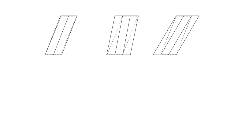
Figure 2: Possible directional adjustments are illustrated for a parallelogram $P$ (dashed line). (a): rule (iii) of Section 2 yields two parallelograms with the same “direction”. (b), (c): applying rule (i) twice, changes the anisotropic direction slightly. The three refined parallelograms depicted in (b), (c) illustrate the results of a possible merging of adjacent triangles.

Figure 3(a), (b) show the adaptive grids associated with the trial space $X_{5}$ and the test space $V_{5}$. The refinement in the neighborhood of the discontinuity curve reflects a highly anisotropic structure. Figure 3(c) illustrates the approximation given by 306 basis elements. We emphasize that the solution is very smooth in the vicinity of the discontinuity curve and oscillations across the jump are almost completely absent and in fact much less pronounced than observed for isotropic discretizations. Figure 3(d) indicates the optimal rate realized by our scheme, see Theorem 2.1.

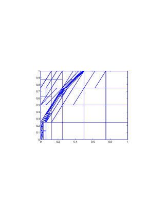
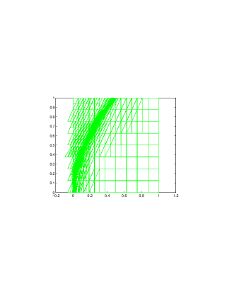
Figure 3: (a) Adaptive grid for the trial space $X_{5}$. (b) Adaptive grid for the test space $V_{5}$. (c) Approximate solution (306 basis elements). (d) $L^{2}(D)$ errors (vertical axis) for $N$ degrees of freedom (horizontal axis) achieved by the adaptive scheme (blue) in comparison with the optimal rate $N^{-1}$ (red), predicted by Theorem 2.1. This is to be compared with the rate $N^{-1/2}$ realized by adaptive isotropic refinements dahmen_huang_kutyniok_lim_schwab:DaHuScWe12 .

The estimated values of the proximality parameter $\delta$, displayed in Table 1, indicate the numerical stability of the scheme.

$n$	Estimated $\delta$	$\|u_{j}^{K}-u\|_{L_{2}([0,1]^{2})}$
48	0.298138	0.036472
99	0.442948	0.021484
138	0.352767	0.013948
177	0.322156	0.010937
237	0.316545	0.008348
306	0.307965	0.006152

Table 1: Numerical estimates (37) for the proximality constant $\delta$ and for the $L_{2}$ approximation error.

In the remainder of the paper we discuss parametric equations whose solutions are functions of spatial variables and additional parameters. Particular attention will here be paid to the radiative transfer problems, where the dimension of the physical domain is $2$ or $3$.

4 Reduced Basis Methods

4.1 Basic Concepts and Rate Optimality

Model reduction is often necessary when solutions to parametric families of PDEs are frequently queried for different parameter values e.g. in an online design or optimization process. The linear transport equation (17) is a simple example of such a parameter dependent PDE. Since a) propagation of singularities is present and b) the parameters determine the propagation direction $\vec{s}$ it turns out to already pose serious difficulties for standard model reduction techniques.

We emphasize that, rather than considering a single variational formulation for functions of spatial variables and parameters, as will be done later in Section 5, we take up the parametric nature of the problem by considering a parametric family of variational formulations. That is, for each fixed $\vec{s}$ the problem is an ordinary linear transport problem for which we can employ the corresponding variational formulation from Section 3.2, where now the respective spaces may depend on the parameters. In this section we summarize some of the results from dahmen_huang_kutyniok_lim_schwab:DePeWo13 which are based in an essential way on the concepts discussed in the previous section.

In general, consider a familiy

$$b_{\mu}(u,v)=f(v),\quad u\in X_{\mu},\,v\in Y_{\mu},\,\,\mu\in\mathcal{P},\,\,b_{\mu}(u,v)=\sum_{k=1}^{M}\Theta_{k}(\mu)b_{k}(u,v)$$ (38)

of well-posed problems, where $\mathcal{P}\subset\mathbb{R}^{P}$ is a compact set of parameters $\mu$, and the parameter dependence is assumed to be affine with smooth functions $\Theta_{k}$. The solutions $u(\cdot;\mu)=u(\mu)$ then become functions of the spatial variables and of the parameters $\mu\in\mathcal{P}$.

As before we can view (38) as a parametric family of operator equations $B_{\mu}u=f$, where $B_{\mu}:X_{\mu}\to Y_{\mu}^{\prime}$ is again given by $(B_{\mu}u)(v)=b_{\mu}(u,v)$. Each particular solution $u(\mu)$ is a point on the solution manifold

$$\mathcal{M}:=\{B_{\mu}^{-1}f:\mu\in\mathcal{P}\}.$$ (39)

Rather than viewing $u(\mu)$ as a point in a very high-dimensional (in fact infinite dimensional) space, and calling a standard solver for each evaluation in a frequent query problem, the Reduced Basis Method (RBM) tries to exploit the fact that each $u(\mu)$ belongs to a much smaller dimensional manifold $\mathcal{M}$. Assuming that all the spaces $X_{\mu}$ are equivalent to a reference Hilbert space $X$ with norm $\|\cdot\|_{X}$, the key objective of the RBM is to construct a possibly small dimensional linear space $X_{n}\subset X$ such that for a given target accuracy $\epsilon>0$

$$\sup_{\mu\in\mathcal{P}}\inf_{w\in X_{n}}\|u(\mu)-w\|_{X}:={\rm maxdist}_{X}(\mathcal{M},X_{n})\leq\epsilon.$$ (40)

Once $X_{n}$ has been found, bounded linear functionals of the exact solution $u(\mu)$ can be approximated within accuracy $\epsilon$ by the functional applied to an approximation from $X_{n}$ which, when $n$ is small, can hopefully be determined at very low cost. The computational work in an RBM is therefore divided into an offline and an online stage. Finding $X_{n}$ is the core offline task which is allowed to be computationally (very) expensive. More generally, solving problems in the “large” space $X$ is part of the offline stage. Of course, solving a problem in $X$ is already idealized. In practice $X$ is replaced by a possibly very large trial space, typically a finite element space, which is referred to as the truth space and should be chosen large enough to guarantee the desired target accuracy, ideally certified by a posteriori bounds.

The computation of a (near-)best approximation $u_{n}(\mu)\in X_{n}$ is then to be online feasible. More precisely, one seeks to obtain a representation

$$u_{n}(\mu)=\sum_{j=1}^{n}c_{j}(\mu)\phi_{j},$$ (41)

where the $\phi_{j}$ form a basis for $X_{n}$ and where for each query $\mu\in\mathcal{P}$ the expansion coefficients $c_{j}(\mu)$ can be computed by solving only problems of the size $n$, see e.g. dahmen_huang_kutyniok_lim_schwab:SeVeHuDeNgPa06 for principles of practical realizations. Of course, such a concept pays off when the dimension $n=n(\epsilon)$, needed to realize (40), grows very slowly when $\epsilon$ decreases. This means that the elements of $\mathcal{M}$ have sparse representations with respect to certain problem dependent dictionaries.

The by now most prominent strategy for constructing “good” spaces $X_{n}$ can be sketched as follows. Evaluating for a given $X_{n}$ the quantity ${\rm maxdist}_{X}(\mathcal{M},X_{n})$ is infeasible because this would require to determine for each $\mu\in\mathcal{P}$ (or for each $\mu$ in a large training set $\mathcal{P}_{h}\subset\mathcal{P}$ which for simplicity we also denote by $\mathcal{P}$) the solution $u(\mu)$ which even for the offline stage is way too expensive. Therefore, one chooses a surrogate $R_{n}(\mu)$ such that

$$\inf_{w\in X_{n}}\|u(\mu)-w\|_{X}\leq R_{n}(\mu,X_{n}),\quad\mu\in\mathcal{P},$$ (42)

where the evaluation of $R_{n}(\mu,X_{n})$ is fast and an optimization of $R_{n}(\mu,X_{n})$ can therefore be performed in the offline stage. This leads to the greedy algorithm in Algorithm 2.

Algorithm 2 greedy algorithm

1:function GA

2:     Set $X_{0}:=\{0\}$, $n=0$,

3:     while ${\rm argmax}_{\mu\in\mathcal{P}}R(\mu,X_{n})\geq\epsilon$ do

4:         

$$\begin{array}[]{ll}\mu_{n+1}&:={\rm argmax}_{\mu\in\mathcal{P}}R(\mu,X_{n}),\\ u_{n+1}&:=u(\mu_{n+1}),\\ X_{n+1}&:={\rm span}\,\big{\{}X_{n},\{u(\mu_{n+1})\}\big{\}}={\rm span}\,\{u_{1},\dots,u_{n+1}\}\end{array}$$ (43)

5:     end while

6:end function

A natural question is to ask how the spaces $X_{n}$ constructed in such a greedy fashion compare with “best spaces” in the sense of the Kolmogorov $n$-widths

$$d_{n}(\mathcal{M})_{X}:=\inf_{{\rm dim}\,W_{n}=n}\sup_{w\in cM}\inf_{z\in W_{n}}\|w-z\|_{X}\;.$$ (44)

The $n$-widths are expected to decay the faster the more regular the dependence of $u(\mu)$ is on $\mu$. In this case an RBM has a chance to perform well.

Clearly, one always has $d_{n}(\mathcal{M})_{X}\leq{\rm maxdist}_{X}(\mathcal{M},X_{n})$. Unfortunately, the best constant $C_{n}$ for which ${\rm maxdist}_{X}(\mathcal{M},X_{n})\leq C_{n}d_{n}(\mathcal{M})_{X}$ is $C_{n}=2^{n}$, see dahmen_huang_kutyniok_lim_schwab:BiCoDaDePeWo11 ; dahmen_huang_kutyniok_lim_schwab:BuMaPa12 . Nevertheless, when comparing rates rather than individual values, one arrives at more positive results dahmen_huang_kutyniok_lim_schwab:BiCoDaDePeWo11 ; dahmen_huang_kutyniok_lim_schwab:DePeWo13-2 . The following consequence of these results asserts optimal performance of the greedy algorithm provided that the surrogate sandwiches the error of best approximation dahmen_huang_kutyniok_lim_schwab:DePeWo13 .

Theorem 4.1

Assume that there exists a constant $0<c_{R}\leq 1$ such that for all $n$ holds

$$c_{R}R_{n}(\mu,X_{n})\leq\inf_{w\in X_{n}}\|u(\mu)-w\|_{X}\leq R_{n}(\mu,X_{n}),\quad\mu\in\mathcal{P}.$$ (45)

Then, the spaces $X_{n}$ produced by Algorithm 2 satisfy

$$d_{n}(\mathcal{M})_{x}\leq Cn^{-\alpha}\quad\Longrightarrow\quad{\rm maxdist}_{X}(\mathcal{M},X_{n})\leq\bar{C}n^{-\alpha},$$ (46)

where $\bar{C}$ depends only on $C,\alpha$, and $\kappa(R_{n}):=1/c_{R}$, the condition of the surrogate.

We call the RBM rate-optimal whenever (46) holds for any $\alpha>0$. Hence, finding rate-optimal RBMs amounts to finding feasible well-conditioned surrogates.

4.2 A Double Greedy Method

Feasible surrogates that do not require the explicit computation of truth solutions for each $\mu\in\mathcal{P}$ need to be based in one way or the other on residuals. When (38) is a family of uniformly $X$-elliptic problems so that $B_{\mu}$ are uniformly bounded isomorphisms from $X$ onto $X^{\prime}$, residuals indeed lead to feasible surrogates whose condition depends on the ratio of the continuity and coercivity constant. This follows from the mapping property of $B_{\mu}$, stability of the Galerkin method, and the best approximation property of the Galerkin projection, see dahmen_huang_kutyniok_lim_schwab:DePeWo13 .

When the problems (38) are indefinite or unsymmetric and singularly perturbed these mechanisms no longer work in this way, which explains why the conventional RBMs do not perform well for transport dominated problems in that they are far from rate-optimal.

As shown in dahmen_huang_kutyniok_lim_schwab:DePeWo13 , a remedy is offered by the above renormation principle providing well-conditioned variational formulations for (38). In principle, these allow one to relate errors (in a norm of choice) to residuals in a suitably adapted dual norm which are therefore candidates for surrogates. The problem is that, given a trial space $X_{n}$, in particular a space generated in the context of an RBM, it is not clear how to obtain a sufficiently good test space such that the corresponding Petrov-Galerkin projection is comparable to the best approximation. The new scheme developed in dahmen_huang_kutyniok_lim_schwab:DePeWo13 is of the following form:

• Initialization: take $X_{1}:={\rm span}\,\{u(\mu_{1})\}$, $\mu_{1}$ randomly chosen, $Y_{1}:=\{0\}$;

• given a pair of spaces $X_{n},\tilde{V}_{n}$, the routine Update-inf-sup-$\delta$ enriches $\tilde{V}_{n}$ to a larger space $V_{n}$ which is $\delta$-proximal for $X_{n}$;

• extend $X_{n}$ to $X_{n+1}$ by a greedy step according to Algorithm 2, set $\tilde{V}_{n+1}=V_{n}$, and go to (II) as long as a given target tolerance for an a posteriori threshold is not met.

The rountine Update-inf-sup-$\delta$ works roughly as follows (see also dahmen_huang_kutyniok_lim_schwab:GeVe12 in the case of the Stokes system). First, we search for a parameter $\bar{\mu}\in\mathcal{P}$ and a function $\bar{w}\in X_{n}$ for which the inf-sup condition is worst, i.e.

$$\sup_{v\in\tilde{V}_{n}}\frac{b_{\bar{\mu}}(\bar{{w}},v)}{\|v\|_{Y_{\bar{\mu}}}\|\bar{{w}}\|_{\hat{X}_{\bar{\mu}}}}=\inf_{\mu\in\mathcal{P}}\left(\inf_{w\in X_{n}}\sup_{v\in\tilde{V}_{n}}\frac{b_{\mu}(w,v)}{\|v\|_{Y_{\mu}}\|{w}\|_{\hat{X}_{\mu}}}\right).$$ (47)

If this worst case inf-sup constant does not exceed yet a desired uniform lower bound, $\tilde{V}_{n}$ does not contain an effective supremizer, i.e., a function realizing the supremum in (47), for $\bar{\mu},\bar{w}$, yet. However, since the truth space satisfies a uniform inf-sup condition, due to the same variational formulation, there exists a good supremizer in the truth space which, is given by the Galerkin problem

$$\bar{v}=R_{Y_{\bar{\mu}}}^{-1}B_{\bar{\mu}}\bar{w}={\rm argmax}_{v\in Y_{\bar{\mu}}}\frac{b_{\bar{\mu}}(\bar{w},v)}{\|v\|_{Y_{\bar{\mu}}}\|\bar{w}\|_{\hat{X}_{\bar{\mu}}}},$$

providing the enrichment $\tilde{V}_{n}\to{\rm span}\{\tilde{V}_{n},R_{Y_{\mu}}^{-1}B_{\mu}\bar{w}\}$.

The interior greedy stabilization loop (II) ensures that the input pair $X_{n},Y_{n}$ in step (III) is inf-sup stable with an inf-sup constant as close to one as one wishes, depending on the choice of $\delta<1$. By Theorem 3.1, each solution $u_{n}(\mu)$ of the discretized system for $(X_{h},V)=(X_{n},V_{n})$ satisfies the near-best approximation property (26), (27). Hence $\|f-B_{\mu}u_{n}(\mu)\|_{Y_{\mu}^{\prime}}$ is a well conditioned surrogate (with condition close to one). Therefore, the assumptions of Theorem 4.1 hold so that the outer greedy step (III) yields a rate-optimal update. In summary, under the precise assumptions detailed in dahmen_huang_kutyniok_lim_schwab:DePeWo13 , the above double greedy scheme is rate-optimal.

Before turning to numerical examples, a few comments on the interior greedy loop Update-inf-sup-$\delta$ are in order.

(a) Finding $\bar{\mu}$ in (47) requires for each $\mu$-query to perform a singular value decomposition in the low dimensional reduced spaces so that this is offline feasible, see (dahmen_huang_kutyniok_lim_schwab:DePeWo13, , Remark 4.2).

(b) When the test spaces $Y_{\mu}$ all agree with a reference Hilbert space $Y$ as sets and with with equivalent norms it is easy to see that the interior stabilization loop terminates after at most $M$ steps where $M$ is the number of parametric components in (38), see (dahmen_huang_kutyniok_lim_schwab:DePeWo13, , Remark 4.9) and dahmen_huang_kutyniok_lim_schwab:GeVe12 ; dahmen_huang_kutyniok_lim_schwab:RoVe07 . If, on the other hand, the spaces $Y_{\mu}$ differ even as sets, as in the case of transport equations when the transport direction is the parameter, this is not clear beforehand. By showing that the inf-sup condition is equivalent to a $\delta$-proximality condition one can show under mild assumptions though that the greedy interior loop still terminates after a number of steps which is independent of the truth dimension, (dahmen_huang_kutyniok_lim_schwab:DePeWo13, , Remark 4.11).

(c) In this latter case the efficient evaluation of $\|f-B_{\mu}u(\mu)\|_{Y_{\mu}^{\prime}}$ requires additional efforts, referred to as iterative tightening, see (dahmen_huang_kutyniok_lim_schwab:DePeWo13, , Section 5.1).

(d) The renormation strategy saves an expensive computation of stability constants as in conventional RBMs since, by construction, through the choice of $\delta$, the stability constants can be driven as close to one as one wishes.

The scheme has been applied in dahmen_huang_kutyniok_lim_schwab:DePeWo13 to convection-diffusion and pure transport problems where the convection directions are parameter dependent. Hence the variational formulations are of the form (38). We briefly report some results for the transport problem, since this is an extreme case in the following sense. The test spaces $Y_{\mu}$ do not agree as sets when one would like the $X_{\mu}$ to be equivalent for different parameters. Hence, one faces the obstructions mentioned in (b), (c) above. Moreover, for discontinuous right hand side and discontinuous boundary conditions the dependence of the solutions on the parameters has low regularity so that the $n$-widths do not decay as rapidly as in the convection-diffusion case. Nevertheless, the rate-optimality still shows a relatively fast convergence for the reduced spaces $X_{n}$ shown below.

The first example concerns (17) (with $\mu=\vec{s}$ ranging over a quarter circle, $D=(0,1)^{2}$) for $f_{\circ}\equiv 1$, $g\equiv 0$. In the second example, we take $f_{\circ}(x_{1},x_{2})=0.5$ for $x_{1}<x_{2}$, $f_{\circ}(x_{1},x_{2})=1$ for $x_{1}\geq x_{2}$.

dimension			maximal	maximal error between		surr /
trial	test	$\delta$	surr	rb truth	rb $L_{2}$	err
4	11	3.95e-01	8.44e-03	2.45e-02	2.45e-02	3.45e-01
10	33	4.32e-01	3.37e-03	5.74e-03	5.74e-03	5.87e-01
16	57	4.32e-01	1.50e-03	2.56e-03	2.56e-03	5.84e-01
20	74	4.16e-01	1.21e-03	2.10e-03	2.10e-03	5.77e-01
24	91	4.05e-01	7.27e-04	1.58e-03	1.58e-03	4.61e-01

Table 2: Numerical results for Example 1, maximal $L_{2}$ truth error 0.000109832.

dimension			maximal	maximal error between		surr /
trial	test	$\delta$	surr	rb truth	rb $L_{2}$	err
first reduced basis creation
20	81	3.73e-01	2.71e-02	5.46e-02	5.62e-02	4.82e-01
second reduced basis creation
10	87	3.51e-01	6.45e-02	7.40e-02	7.53e-02	8.57e-01

Table 3: Numerical results for Example 2 after a single cycle of iterative tightening. Maximal $L_{2}$ truth error 0.0154814

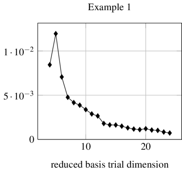
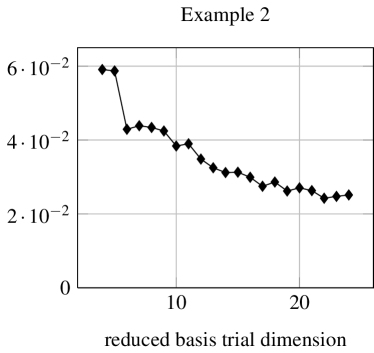
Figure 4: Surrogates of the reduced basis approximation for Examples 1 and 2.

5 Sparse Tensor Approximation for Radiative Transfer

We now extend the parametric transport problem (17) to the radiative transport problem (RTP) (see, eg., dahmen_huang_kutyniok_lim_schwab:Mo03 ) which consists in finding the radiative intensity $u:D\times\mathcal{S}\rightarrow\mathbb{R}$, defined on the Cartesian product of a bounded physical domain $D\subset\mathbb{R}^{d}$, where $d=2,3$, and the unit $d_{\mathbb{S}}$-sphere as the parameter domain: $\mathcal{P}=\mathcal{S}$ with $d_{\mathbb{S}}=1,2$. Given an absorption coefficient $\kappa\geq 0$, a scattering coefficient $\sigma\geq 0$, and a scattering kernel or scattering phase function $\Phi>0$, which is normalized to $\int_{\mathcal{S}}\Phi(\vec{s},\vec{s}^{\prime}){\rm d}{\vec{s}^{\prime}}=1$ for each direction $\vec{s}$, one defines the transport operator $\mathrm{T}u:=(\vec{s}\cdot{\boldmath\nabla}_{x}+\kappa)u$, and the scattering operator $\mathrm{Q}u:=\sigma\mathrm{Q_{1}}\!u=\sigma(u-\int_{\mathcal{S}}\Phi(\vec{s},\vec{s}^{\prime})u(\vec{x},\vec{s}^{\prime}){\rm d}{\vec{s}^{\prime}})$. The radiative intensity is then given by

$$(\mathrm{T}+\mathrm{Q})u=f,\;\;u|_{\partial\Omega_{-}}=g,$$ (48)

where $f:=\kappa I_{b}$, $\partial\Omega_{-}:=\{(\vec{x},\vec{s})\in\partial D\times\mathcal{S}:\vec{s}\cdot\vec{n}(\vec{x})<0\}$, and $g$ denote the source term, the inflow-boundary, and the inflow-boundary values, respectively. As before, $\Gamma_{-}(\vec{s}):=\{\vec{x}\in\partial D:\vec{s}\cdot\vec{n}(\vec{x})<0\}$ stands for the physical inflow-boundary.

The partial differential equation (48) is known as stationary monochromatic radiative transfer equation (RTE) with scattering, and can be viewed as (nonlocal) extension of the parametric transport problem (17), where the major difference to (17) is the scattering operator $Q$. Sources with support contained in $D$ are modeled by the blackbody intensity $I_{b}\geq 0$, radiation from sources outside of the domain or from its enclosings is prescribed by the boundary data $g\geq 0$. The vector $\vec{n}(\vec{x})$ denotes the outer unit normal on the boundary $\partial D$ of the physical domain.

Deterministic numerical methods for the RTP which are commonly used in engineering comprise the discrete ordinates ($S_{N}$-) method and the spherical harmonics ($P_{N}$-) method.

In the discrete ordinate method (DOM), the angular domain is collocated by a finite number of fixed propagation directions in the angular parameter space; in this respect, the DOM resembles the greedy collocation in the parameter domain: each of the directions Eq. (48) results in a spatial PDE which is solved (possibly in parallel) by standard finite differences, finite elements, or finite volume methods.

In the spherical harmonics method (SHM), a spectral expansion with spatially variable coefficients is inserted as ansatz into the variational principle Eq. (48). By orthogonality relations, a coupled system of PDEs (whose type can change from hyperbolic to elliptic in the so-called diffuse radiation approximation) for the spatial coefficients is obtained, which is again solved by finite differences or finite elements.

The common deterministic methods $S_{N}$- and $P_{N}$-approximation exhibit the so-called “curse of dimensionality”: the error with respect to the total numbers of degrees of freedom (DoF) $M_{D}$ and $M_{\mathcal{S}}$ on the physical domain $D$ and the parameter domain $\mathcal{S}$ scales with the dimension $d$ and $d_{\mathbb{S}}$ as $O(M_{D}^{-s/d}+M_{\mathcal{S}}^{-t/d_{\mathbb{S}}})$ with positive constants $s$ and $t$.

The so called sparse grid approximation method alleviates this curse of dimensionality for elliptic PDEs on cartesian product domains, see dahmen_huang_kutyniok_lim_schwab:BuGr04 and the references therein. dahmen_huang_kutyniok_lim_schwab:WiHiSc08 has developed a sparse tensor method to overcome the curse of dimensionality for radiative transfer with a wavelet (isotropic) discretization of the angular domain. Under certain regularity assumptions on the absorption coefficient $\kappa$ and the blackbody intensity $I_{b}$, their method achieves the typical benefits of sparse tensorization: a log-linear complexity in the number of degrees of freedom of a component domain with an essentially (up to a logarithmic factor) undeteriorated rate of convergence. However, scattering had not been addressed in that work.

In order to include scattering and to show that the concepts of sparse tensorization can also be applied to common solution methods, sparse tensor versions of the spherical harmonics approximation were developed extending the “direct sparse” approach by dahmen_huang_kutyniok_lim_schwab:WiHiSc08 . The presently developed version also accounts for scattering dahmen_huang_kutyniok_lim_schwab:GrSc11a . For this sparse spherical harmonics method, we proved that the benefits of sparse tensorization can indeed be harnessed.

As a second method a sparse tensor product version of the DOM based on the sparse grid combination technique was realized and analyzed in dahmen_huang_kutyniok_lim_schwab:Gr13 ; dahmen_huang_kutyniok_lim_schwab:GrSc11b . Solutions to discretizations of varying discretization levels, for a number of collocated transport problems, and with scattering discretized by combined Galerkin plus quadrature approximation in the transport collocation directions are combined in this method to form a sparse tensor solution that we proved in dahmen_huang_kutyniok_lim_schwab:Gr13 ; dahmen_huang_kutyniok_lim_schwab:GrSc11b breaks the curse of dimensionality as described above. These benefits hold as long as the exact solution of the RTE is sufficiently regular. An overview follows.

5.1 Sparse discrete ordinates method (Sparse DOM)

We adopt a formulation where the inflow boundary conditions are enforced in a weak sense. To this end, we define the boundary form (see, eg., dahmen_huang_kutyniok_lim_schwab:Gr13 )

$$\partial b(u,v):={(v,\vec{s}\cdot\vec{n}u)}_{L^{2}(\partial\Omega_{-})}=\int_{\mathcal{S}}\int_{\Gamma_{-}(\vec{s})}\vec{s}\cdot\vec{n}uv{\rm d}{\vec{x}}{\rm d}{\vec{s}}\;.$$ (49)

For $v:D\times\mathcal{S}\rightarrow\mathbb{R}$, the norms

$$\|v\|_{-}^{2}:=-\partial b(v,v),\quad{\|v\|_{1}}^{2}:=\|v\|^{2}+\|\vec{s}\cdot{\boldmath\nabla}_{x}v\|^{2}+\|\mathrm{Q_{1}}\!v\|^{2}+\|v\|_{-}^{2}$$

define the Hilbert space $\mathcal{V}_{1}:=\{v\in L^{2}(D\times\mathcal{S}):\|v\|_{1}<\infty\}$  . The SUPG-stabilized Galerkin variational formulation reads: find $u\in\mathcal{V}_{1}$ such that

$$({\mathrm{R}v},{(\mathrm{T}+\mathrm{Q})u})_{L^{2}({D\times\mathcal{S}})}-2\partial b(u,v)=({\mathrm{R}v},{f})_{L^{2}(D\times\mathcal{S})}-2\partial b(g,v)\quad\forall v\in\mathcal{V}_{1}$$ (50)

with SUPG stabilization $\mathrm{R}v:=v+\delta\vec{s}\cdot{\boldmath\nabla}_{x}v$, where $\delta\approx 2^{-L}$.

For the discretization of (50), we replace $\mathcal{V}_{1}$ by $V^{L,N}=V_{D}^{L}\otimes V_{\mathcal{S}}^{N}$. In the physical domain, standard $P_{1}$-FEM with a one-scale basis on a uniform mesh of width $h_{\max}\lesssim 2^{-L}$ is used, in the angular domain, piecewise constants on a quasiuniform mesh of width $h_{\max}\lesssim N^{-1}$. Fully discrete problems are obtain with a one-point quadrature in the angular domain. The resulting Galerkin formulation (50) can be shown to result in the same linear system of equations as the standard collocation discretization (dahmen_huang_kutyniok_lim_schwab:Gr13, , Sec. 5.2). The solution is constructed with the sparse grid combination technique (cp. dahmen_huang_kutyniok_lim_schwab:BuGr04 :

$$\hat{u}_{L,N}=\sum_{\ell_{D}=0}^{L}\left(u_{\ell_{D},\ell_{\mathcal{S}}^{\max}(\ell_{D})}-u_{\ell_{D},\ell_{\mathcal{S}}^{\max}(\ell_{D}+1)}\right),$$

where $u_{\ell_{D},\ell_{\mathcal{S}}}\in V^{\ell_{D},\ell_{\mathcal{S}}}$ denotes the solution to a full tensor subproblem of physical resolution level $\ell_{D}$ and angular resolution level $\ell_{\mathcal{S}}$. The maximum angular index $\ell_{\mathcal{S}}^{\max}=2^{\lfloor\log_{2}(N+1)\rfloor/L(L-l_{D})}$ ensures that the angular resolution decreases when the physical resolution increases and vice versa.

While the full tensor solution $u_{L,N}$ requires $O(2^{dL}N^{d_{\mathbb{S}}})$ degrees of freedom, the sparse solution involves asymptotically at most $O((L+\log N)(2^{dL}+N^{d_{\mathbb{S}}}))$ degrees of freedom (dahmen_huang_kutyniok_lim_schwab:Gr13, , Lemma 5.6). At the same time,

$$\|u-u_{L,N}\|_{1}\lesssim 2^{-L}\|u\|_{H^{2,0}(D\times\mathcal{S})}+N^{-1}\|u\|_{H^{1,1}(D\times\mathcal{S})},$$

while for solutions in $H^{2,1}(D\times\mathcal{S})\subset(H^{2,0}(D\times\mathcal{S})\cap H^{1,1}(D\times\mathcal{S}))$

$$\|u-\hat{u}_{L,N}\|_{1}\lesssim L\max\{2^{-L},N^{-1}\}\|u\|_{H^{2,1}(D\times\mathcal{S})}\;.$$

5.2 Numerical experiment

To evaluate the solution numerically we monitor the incident radiation $G(\vec{x})=\int_{\mathcal{S}}u(\vec{x},\vec{s})\mbox{d}\vec{s}$ and its relative error $err(G_{L,N})_{X}=\|G-G_{L,N}\|_{X}/\|G\|_{X}$, $X=L^{2}(D),H^{1}(D)$.

The setting for the experiment is $D=[0,1]^{d}$, $\mathcal{S}=\mathcal{S}^{d}_{\mathbb{S}}$. We solve the RTP (48) with isotropic scattering $\Phi(\vec{s},\vec{s}^{\prime})=1/|\mathcal{S}|$ and with zero inflow boundary conditions $g=0$. A blackbody radiation $I_{b}(\vec{x},\vec{s})$ corresponding to the exact solution

$$u(\vec{x},\vec{s})=\frac{3}{16\pi}(1+(\vec{s}\cdot\vec{s}^{\prime})^{2})\prod_{i=1}^{3}(-4x_{i}(x_{i}-1)),$$

with fixed $\vec{s}^{\prime}=(1/\sqrt{3},1/\sqrt{3},1/\sqrt{3})^{\top}$ is inserted in the right hand side functional in (50). The absorption coefficient is set to $\kappa=1$, the scattering coefficient to $\sigma=0.5$.

This $3+2$-dimensional problem was solved with a parallel C++ solver designed for the sparse tensor solution of large-scale radiative transfer problems.

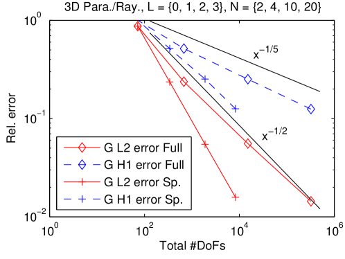
Figure 5: Convergence in incident radiation with full and sparse DOM. Resolution for reference solution was $L_{\mbox{ref}}=4$. Reference slopes provided as visual aids only.

Fig. 5 shows the superior efficiency of the sparse approach with respect to number of degrees of freedom vs. achieved error. The convergence rates indicate that the curse of dimensionality is mitigated by the sparse DOM. Further gains are expected once the present, nonadaptive sparse DOM is replaced by the greedy versions outlined in Section 3.1.

References

- (1) Bachmayer, M., Dahmen, W.: Adaptive near-optimal rank tensor approximation for high-dimensional operator equations. http://arxiv.org/submit/851475, 2013, to appear in Journal of Foundations of Computational Mathematics.
- (2) Barrett, J.W., Morton, K.W.: Approximate symmetrization and Petrov-Galerkin methods for diffusion-convection problems. Comput. Method. Appl. M. 45, 97–12 (1984)
- (3) Binev, P., Cohen, A., Dahmen, W., DeVore, R., Petrova, G., Wojtaszczyk, P.: Convergence Rates for Greedy Algorithms in Reduced Basis Methods. SIAM J. Math. Anal. 43, 1457–1472 (2011)
- (4) Bochev, P.B., Gunzburger, M.D.: Least-Squares Finite Element Methods. Applied Mathematical Sciences, Springer-Verlag (2009)
- (5) Buffa, A., Maday, Y., Patera, A.T., Prud’homme, C., Turinici, G.: A Priori convergence of the greedy algorithm for the parameterized reduced basis. ESAIM-Math. Model. Num. 46, 595–603 (2012)
- (6) Bungartz, H.-J., Griebel, M.: Sparse grids. In: A. Iserles, editor, Acta numerica, vol. 13, pp. 147–269. Cambridge University Press (2004)
- (7) Cai, Z., Manteuffel, T., McCormick, S., Ruge, J.: First-order system : scalar elliptic partial differential equtions. SIAM J. Numer. Anal. 39, 1418–1445 (2001)
- (8) Candès, E.J., Donoho, D.L.: New tight frames of curvelets and optimal representations of objects with piecewise- singularities. Comm. Pure Appl. Math. 57, 219–266 (2002)
- (9) Chen, L., Sun, P., Xu, J.: Optimal anisotropic simplicial meshes for minimizing interpolation errors in norm. Math. Comput. 76, 179–204 (2007)
- (10) Chkifa, A., Cohen, A., DeVore, R., Schwab, C.: Adaptive algorithms for sparse polynomial approximation of parametric and stochastic elliptic PDEs. M2AN Math. Mod. and Num. Anal. 47, 253–280 (2013)
- (11) Cohen, A., DeVore, R., Schwab, C.: Convergence rates of best -term Galerkin approximations for a class of elliptic sPDEs. Found. Comput. Math. 10, 615–646 (2010)
- (12) Cohen, A., Dyn, N., Hecht, F., Mirebeau, J.-M.: Adaptive multiresolution analysis based on anisotropic triangulations. Math. Comput. 81, 789–810 (2012)
- (13) Cohen, A., Dahmen, W., Welper, G.: Adaptivity and Variational Stabilization for Convection-Diffusion Equations. ESAIM-Math. Model. Num. 46, 1247–1273 (2012)
- (14) Cohen, A., Mirebeau, J.-M.: Greedy bisection generates optimally adapted triangulations. Math. Comput. 81, 811–837 (2012)
- (15) Cohen, A., Mirebeau, J.-M.: private communication, 2013
- (16) Dahmen, W., Huang, C., Schwab, C., Welper, G.: Adaptive Petrov-Galerkin methods for first order transport equations. SIAM J. Numer. Anal. 50, 2420–2445 (2012)
- (17) Dahmen, W., Kutyniok, G., Lim, W.-Q, Schwab, C., Welper, G.: Adaptive anisotropic discretizations for transport equations. in preparation.
- (18) Dahmen, W., Plesken, C., Welper, G.: Double greedy algorithms: reduced basis methods for transport dominated problems. ESAIM: M2AN, doi 10.1051/m2an/2013103, http://arxiv.org/abs/1302.5072
- (19) Demkowicz, L.F., Gopalakrishnan, J.: A class of discontinuous Petrov-Galerkin Methods I: The transport equation. Comput. Meth. Appl. Mech. Engrg. 199, 1558–1572 (2010)
- (20) Demkowicz, L., Gopalakrishnan, J.: A class of discontinuous Petrov-Galerkin methods. Part II: Optimal test functions. Numer. Meth. Part. D. E. 27, 70–105 (2011).
- (21) DeVore, R., Petrova, G., Wojtaszczyk, P.: Greedy algorithms for reduced bases in Banach spaces. Constr. Approx. 37, 455–466 (2013)
- (22) Dolejsi, V.: Anisotropic mesh adaptation for finite volume and finite element methods on triangular meshes. Comput. Vis. Sci. 1, 165–178 (1998)
- (23) Donoho, D.L.: Sparse components of images and optimal atomic decompositions. Constr. Approx. 17, 353–382 (2001)
- (24) Donoho, D.L., Kutyniok, G.: Microlocal Analysis of the Geometric Separation Problem. Comm. Pure Appl. Math. 66, 1–47 (2013)
- (25) Gerner, A., Veroy-Grepl, K.: Certified reduced basis methods for parametrized saddle point problems. SIAM J. Sci. Comput. 35, 2812–2836 (2012)
- (26) Grella, K., Schwab, C.: Sparse tensor spherical harmonics approximation in radiative transfer. J. Comput. Phys. 230, 8452–8473 (2011)
- (27) Grella, K., Schwab, C.: Sparse Discrete Ordinates Method in Radiative Transfer. Comp. Meth. Appl. Math. 11, 305–326 (2011)
- (28) Grella, K.: Sparse tensor approximation for radiative transport. PhD thesis 21388, ETH Zurich (2013)
- (29) King, E.J., Kutyniok, G., Zhuang, X.: Analysis of Inpainting via Clustered Sparsity and Microlocal Analysis. J. Math. Imaging Vis. 48, 205-234 (2014)
- (30) Kutyniok, G., Labate, D.: Resolution of the wavefront set using continuous shearlets. Trans. Amer. Math. Soc. 361, 2719–2754 (2009)
- (31) Kittipoom, P., Kutyniok, G., Lim, W.-Q: Construction of Compactly Supported Shearlet Frames. Constr. Approx. 35, 21–72 (2012)
- (32) Kutyniok, G., Labate, D.: Shearlets: Multiscale Analysis for Multivariate Data. Birkhäuser Boston (2012)
- (33) Kutyniok, G., Lemvig, J., Lim, W.-Q: Optimally Sparse Approximations of 3D Functions by Compactly Supported Shearlet Frames. SIAM J. Math. Anal. 44, 2962–3017 (2012)
- (34) Kutyniok, G., Lim, W.-Q: Compactly Supported Shearlets are Optimally Sparse. J. Approx. Theory 163, 1564–1589 (2011)
- (35) Lim, W.-Q: The discrete shearlet transform: A new directional transform and compactly supported shearlet frames. IEEE Trans. Image Proc. 19,1166–1180 (2010)
- (36) Mirebeau, J.-M. Adaptive and anisotropic finite element approximation: Theory and algorithms, PhD thesis, Université Pierre et Marie Curie - Paris VI (2011) http://tel.archives-ouvertes.fr/tel-00544243
- (37) Modest, M.F.: Radiative Heat Transfer. Elsevier, 2nd edition, Amsterdam (2003)
- (38) Rozza, G., Veroy, K.: On the stability of reduced basis techniques for Stokes equations in parametrized domains. Comput. Method. Appl. M. 196, 1244–1260 (2007)
- (39) Sen, S., Veroy, K., Huynh, D.B.P., Deparis, S., Nguyn, N.C., Patera, A.T.: “Natural norm” a-posteriori error estimators for reduced basis approximations. J. Comput. Phys. 217, 37–62 (2006)
- (40) Widmer, G., Hiptmair, R., Schwab, C.: Sparse adaptive finite elements for radiative transfer. J. Comput. Phys. 227, 6071–6105 (2008).
- (41) Welper, G.: Infinite dimensional stabilization of convection-dominated problems. PhD thesis, RWTH Aachen (2013) http://darwin.bth.rwth-aachen.de/opus3/volltexte/2013/4535/