Spectral and morphological analysis of the remnant of Supernova 1987A
with ALMA & ATCA

Abstract

We present a comprehensive spectral and morphological analysis of the remnant of Supernova (SN) 1987A with the Australia Telescope Compact Array (ATCA) and the Atacama Large Millimeter/submillimeter Array (ALMA). The non-thermal and thermal components of the radio emission are investigated in images from 94 to 672 GHz ($\lambda$ 3.2 mm to 450 $\mu$m), with the assistance of a high-resolution 44 GHz synchrotron template from the ATCA, and a dust template from ALMA observations at 672 GHz. An analysis of the emission distribution over the equatorial ring in images from 44 to 345 GHz highlights a gradual decrease of the east-to-west asymmetry ratio with frequency. We attribute this to the shorter synchrotron lifetime at high frequencies. Across the transition from radio to far infrared, both the synchrotron/dust-subtracted images and the spectral energy distribution (SED) suggest additional emission beside the main synchrotron component ($S_{\nu}\propto\nu^{-0.73}$) and the thermal component originating from dust grains at $T\sim 22$ K. This excess could be due to free-free flux or emission from grains of colder dust. However, a second flat-spectrum synchrotron component appears to better fit the SED, implying that the emission could be attributed to a pulsar wind nebula (PWN). The residual emission is mainly localised west of the SN site, as the spectral analysis yields $-0.4\lesssim\alpha\lesssim-0.1$ across the western regions, with $\alpha\sim 0$ around the central region. If there is a PWN in the remnant interior, these data suggest that the pulsar may be offset westward from the SN position.

1. Introduction

The evolution of the remnant of Supernova (SN) 1987A in the Large Magellanic Cloud has been closely monitored since the collapse of its progenitor star, Sanduleak (Sk) $-69^{\circ}202$, on 1987 February 23. Models of Sk $-69^{\circ}202$ indicated that it had an initial mass of $\sim$20 $M_{\sun}$ (hil87). The mass range of the progenitor is consistent with the formation of a neutron star (thi85), and thus with the neutrino events reported by the KamiokaNDE (hir87) and IMB (bio87; hai88) detectors. Models by cro00 suggest a transition from red supergiant (RSG) into blue supergiant (BSG) to explain the hourglass nebula structure, which envelopes the SN with three nearly-stationary rings (che95; blo93; mar95; mor07). The two outer rings, imaged with the Hubble Space Telescope (HST; jak91; pla95), are located on either side of the central ring in the equatorial plane (equatorial ring, ER), and likely formed at the same time as the ER (cro00; tzi11). The synchrotron emission, generated by the shock propagating into the clumpy circumstellar medium (CSM) close to the equatorial plane, was detected in the mid-90s (tur90; sta92), and has become brighter over time (man02; zan10). Radio observations have stretched from flux monitoring at 843 MHz with the Molonglo Observatory Synthesis Telescope (sta93; bal01) to images of sub-arcsec resolution with the Australia Telescope Compact Array (ATCA) (gae97; man05; ng08; pot09; zan13). ATCA observations at 94 GHz (lak12) have been followed by observations from 100 GHz up to 680 GHz with the Atacama Large Millimeter/submillimeter Array (ALMA; kam13; ind14).

The ongoing shock expansion has been monitored at 9 GHz since 1992 (gae97; gae07). Shock velocities of $\sim$4000 km s^-1 have been measured between day 4000 and 7000 (ng08), while signs of a slower expansion have been tentatively detected after day $\sim$7000, as the shock has likely propagated past the high-density CSM in the ER (ng13). Similar evidence of slower shock expansion since day $\sim$6000 has been found in X-ray data (par05; par06; rac09) as well as in infrared (IR) data (bou06).

Since the early super-resolved images at 9 GHz (gae97), a limb-brightened shell morphology has been characteristic of the remnant. The radio emission, over the years, has become more similar to an elliptical ring rather than the original truncated-shell torus (ng13). The radio remnant has shown a consistent east-west asymmetry peaking on the eastern lobe, which has been associated with higher expansion velocities of the eastbound shocks (zan13). The asymmetry degree appears to have changed with the shock expansion, as images at 9 GHz exhibit a decreasing trend in the east-west asymmetry since day $\sim$7000 (ng13). High-resolution observations at 1.4–1.6 GHz (ng11) via Very Long Baseline Interferometry (VLBI) with the Australian Large Baseline Array (LBA), have highlighted the presence of small-scale structures in the brightest regions in both lobes.

The relation between the radio emission and the synchrotron spectral indices, $\alpha$ ($S_{\nu}\propto\nu^{\alpha}$), has been investigated via both flux monitoring (man02; zan10) and imaging observations (pot09; lak12; zan13) with the ATCA. The progressive flattening of the radio spectrum derived from 843 MHz to 8.6 GHz at least since day 5000, coupled with the $e$-folding rate of the radio emission, has pointed to an increasing production of non-thermal electrons and cosmic rays (CR) by the shock front (zan10). On the other hand, the association of steeper spectral indices with the brightest eastern sites implies a higher injection efficiency on the eastern side of the SNR (zan13). Flatter spectral indices in the center of the remnant have been tentatively identified from low-resolution two-frequency spectral maps (pot09; lak12), while at 18–44 GHz the central and center-north regions have $-0.5\lesssim\alpha\lesssim-0.3$ (zan13). With ALMA, the spectral energy distribution (SED) of the remnant has been mapped where the non-thermal and thermal components of the emission overlap, identifying cold dust in the SNR interior (ind14), which accommodates $0.4-0.7\,M_{\sun}$ of the dust mass discovered with the Herschel Space Observatory (Herschel; mat11) in the ejecta.

This paper combines the results presented by ind14 with a comprehensive morphological and spectral analysis of SNR 1987A based on both ATCA and ALMA data. In § 2, we present the ALMA Cycle 0 super-resolved images before and after subtraction, in the Fourier plane, of the synchrotron and dust components (§ 3). In § 4, we assess the remnant asymmetry from 44 to 345 GHz. In § 5, we update the SED derived by ind14, while, in § 6, we investigate the spectral index variations in the SNR across the transition from radio to far infrared (FIR). In § 7, we discuss possible particle flux injection by a pulsar situated in the inner regions of the remnant.

Table 1ALMA Observing Parameters

Parameter	102 GHz	213 GHz	345 GHz	672 GHz
	(Band 3, B3)	(Band 6, B6)	(Band 7, B7)	(Band 9, B9)
Date (2012)	Apr 5, 6	Jul 15 & Aug 10	Jul 14 & Aug 24	Aug 25 & Nov 5
Day since explosion	9174	9287	9294	9351
Frequency bands (GHz)	100.093–101.949	213.506–213.597	336.979–340.917	661.992–665.992
	102.051–103.907		349.010–352.963	678.008–682.008
Center frequency (GHz)	101.918	213.146	345.364	672.165
Channel width (MHz)	4.883	4.883	31.250	15.625
Max baselines ($u,v$) (k$\lambda$)	150, 120	180, 260	400, 400	700, 700
No. of antennas	14–18	14–23	28	19–25
Total observing time (hr)	0.83	1.03	0.62	3.40

Table 2Image Parameters

Image	$S_{\nu}$	SR Beam	DL Beam	PA	Rms noise	Dynamic range
(GHz)	(mJy)	(′′)	(′′)	(∘)	(mJy/beam)
94	$24.2\pm 3.9$	$0.7$	$\cdots$	$\cdots$	$0.085$	$137$
102	$23.1\pm 3.1$	$0.8$	$1.74\times 1.25$	$5.7$	$0.033$	$285$
213	$19.7\pm 1.6$	$0.6$	$1.16\times 0.74$	$-68.5$	$0.034$	$75$
345	$16.7\pm 1.5$	$0.3$	$0.65\times 0.48$	$-40.2$	$0.023$	$121$
672	$52.8\pm 14.2$	$0.3$	$0.34\times 0.28$	$68.5$	$1.219$	$28$
94$-I_{\rm B9}$	$23.2\pm 3.9$	$0.7$	$0.78\times 0.63$	$15.4$	$0.094$	$81$
102$-I_{\rm B9}$	$19.4\pm 3.2$	$0.8$	$1.66\times 1.19$	$6.3$	$0.034$	$143$
213$-I_{\rm B9}$	$16.9\pm 1.9$	$0.6$	$1.16\times 0.74$	$-68.5$	$0.029$	$64$
345$-I_{\rm B9}$	$11.5\pm 1.9$	$0.3$	$0.65\times 0.48$	$-44.0$	$0.031$	$43$
672$-I_{\rm B9}$	$-1.0\pm 14.3$	$0.3$	$0.34\times 0.28$	$68.5$	$1.193$	$2$
94$-I_{44}$	$0.9\pm 3.9$	$0.7$	$0.78\times 0.63$	$15.4$	$0.095$	$60$
102$-I_{44}$	$3.5\pm 3.1$	$0.8$	$1.48\times 0.96$	$10.1$	$0.027$	$81$
213$-I_{44}$	$2.9\pm 1.7$	$0.6$	$1.16\times 0.74$	$-68.5$	$0.024$	$26$
345$-I_{44}$	$5.8\pm 1.6$	$0.3$	$0.65\times 0.48$	$-44.0$	$0.014$	$90$
672$-I_{44}$	$47.4\pm 14.8$	$0.3$	$0.57\times 0.55$	$78.6$	$0.816$	$24$

.

2. Observations and Analysis

The ATCA and ALMA observations used in this study were performed in 2011 and 2012. ATCA observations at 44 and 94 GHz are detailed in zan13 and lak12, respectively. ALMA observations were made in 2012 (Cycle 0) from April to November, over four frequency bands: Band 3 (B3, 84–116 GHz, $\lambda$ 3 mm), Band 6 (B6, 211–275 GHz, $\lambda$ 1.3 mm), Band 7 (B7, 275–373 GHz, $\lambda$ 850 $\mu$m) and Band 9 (B9, 602–720 GHz, $\lambda$ 450 $\mu$m). Each band was split over dual 2-GHz-wide sidebands, with minimum baselines of 17 m (B9) to maximum baselines of 400 m (B3). All observations used quasars J0538-440 and J0637-752 as bandpass and phase calibrators, respectively. Callisto was observed as an absolute flux calibrator in B3 and B6, while Ceres was used in B7 and B9 (see also kam13). It is noted that, while ALMA is designed to yield data with flux density calibration uncertainty as low as $\sim$1%, in Cycle 0 this uncertainty is estimated at $\sim$5% at all frequencies. Relevant observational parameters are listed in Table 1 (see also Table 1 in ind14).

Each dataset was calibrated with the casa package, then exported in miriad for imaging. After clean-ing (hog74), both phase and amplitude self-calibration were applied in B3 over a 2-minute solution interval, while only phase calibration was applied in B6 and B7. No self-calibration was performed in B9. As in zan13, we note that since the self-calibration technique removes position information, each image was compared with that prior to self-calibration and, in case of positional changes, the self-calibrated images were shifted. Further adjustments were made in the comparison with the ATCA observations at 44 GHz, based on prominent features on the eastern lobe and location of the remnant center. As from zan13, the 44 GHz image was aligned with VLBI observations of the SNR (Zanardo et al. in preparation). Adding in quadrature these positional uncertainties and the accuracy of the LBA VLBI frame, the errors in the final image position are estimated at $\sim$60 mas.

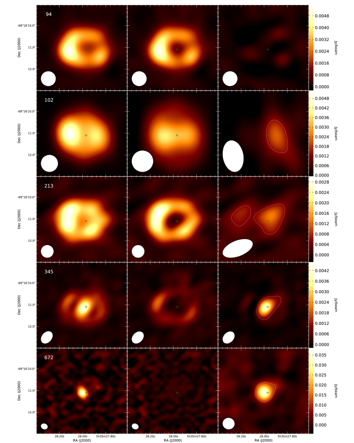
Figure 1.— Top to bottom – Left column: Stokes $I$ continuum images of SNR 1987A at 94 (lak12), 102, 213, 345 and 672 GHz. Images from 102 to 672 GHz are made from ALMA observations (Cycle 0) performed from 2012 April 5 to November 5 (see Table 1). center column: Images obtained by subtracting the model flux density at 672 GHz (Band 9) scaled to fit the central emission. Right column: Images obtained by subtracting a scaled model flux density at 44 GHz (zan13), with $3\,\sigma$ flux density contours highlighted (white). The angular resolution is shown in the bottom left corner. The green cross indicates the VLBI position of SN 1987A as determined by rey95 [RA $05^{\rm h}\;35^{\rm m}\;27\hbox{$.\!\!^{\rm s}$}968$, Dec $-69^{\circ}\;16^{\prime}\;11\hbox{$.\!\!^{\prime\prime}$}09$ (J2000)].

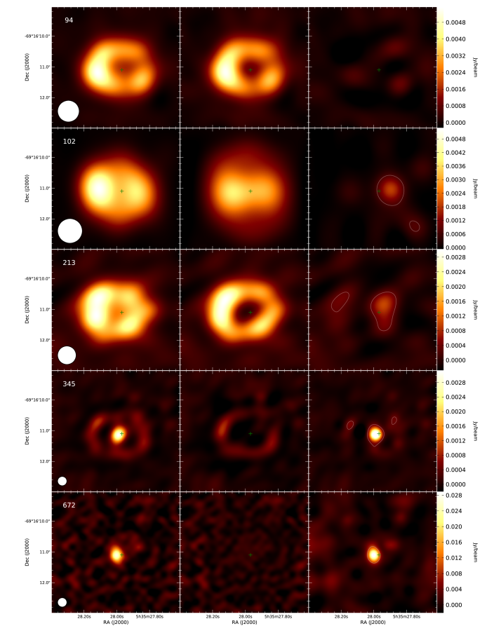
Figure 2.— The panel layout is identical to that in Figure 1, but all Stokes $I$ continuum subtracted images are super-resolved. The circular beam used for the super-resolved ALMA images is $0\hbox{$.\!\!^{\prime\prime}$}8$ at 102 GHz (Band 3), $0\hbox{$.\!\!^{\prime\prime}$}6$ at 213 GHz (Band 6), $0\hbox{$.\!\!^{\prime\prime}$}3$ at 345 (Band 7) and 672 GHz (Band 9), and is plotted in the lower left corner. The 94 GHz images are restored with a $0\hbox{$.\!\!^{\prime\prime}$}7$ circular beam. For images on the right column, $3\,\sigma$ flux density contours are highlighted (white). The green cross indicates the VLBI position of SN 1987A as determined by rey95.

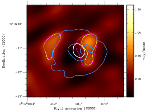
Figure 3.— Stokes $I$ continuum image of SNR 1987A at 213 GHz as obtained after the dual subtraction of the model flux densities at 44 and 672 GHz (see § 2). The image is super-resolved with a 0$.\!\!^{\prime\prime}$6 circular beam, and the yellow contour highlights the $3\,\sigma$ flux density levels. The off-source rms noise is 0.14 mJy beam^-1 (S/N $\sim 6\,\sigma$). For comparison, the 213 GHz image obtained after the single subtraction of the model flux density at 44 GHz and similarly super-resolved with a 0$.\!\!^{\prime\prime}$6 circular beam (see Figure 2), is outlined via the $3\,\sigma$ flux density levels (magenta contours). The model images, i.e. the Stokes $I$ images at 44 GHz (zan13) and at 672 GHz, are outlined by blue and white contours, respectively, at the $5\,\sigma$ flux density levels. Both model images are resolved with a 0$.\!\!^{\prime\prime}$3 circular beam.

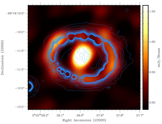
Figure 4.— Overlay of the HST image of SNR 1987A (light blue contours; (lar11)) on the 345 GHz image produced from ALMA observations performed in 2012 June and August (brown–yellow color scale and red contours). As from Figure 2, the ALMA image is super-resolved with a $0\hbox{$.\!\!^{\prime\prime}$}3$ circular beam.

Deconvolution was carried out via the maximum entropy method (MEM) (gul78) in B3, B6 and B7. A weighting parameter of robust = 0.5 (bri95) was used in all bands. The resultant diffraction-limited images, which have central frequency at 102 GHz in B3, 213 GHz in B6, 345 GHz in B7 and 672 GHz in B9, were then super-resolved with a circular beam of $0\hbox{$.\!\!^{\prime\prime}$}8$ in B3, $0\hbox{$.\!\!^{\prime\prime}$}6$ in B6, and $0\hbox{$.\!\!^{\prime\prime}$}3$ in B7 and B9. The diffraction limited and super-resolved images are shown in the first column of Figures 1 and 2, below the ATCA image at 94 GHz (lak12). Integrated Stokes $I$ flux densities, dynamic range and related rms are given in Table  2.

To decouple the non-thermal emission from that originating from dust, the synchrotron component, as resolved with ATCA at 44 GHz (zan13), and the dust component, as imaged with ALMA at 672 GHz (B9) (ind14), were separately subtracted from the datasets at 94, 102, 213, 345 and 672 GHz. All subtractions were performed in the Fourier plane, via miriad task uvmodel, where the model flux density at 44 GHz was scaled to fit the SNR emission over the ER ($I_{44}$), while the B9 model flux density was scaled to fit the emission localised in the central region of the remnant ($I_{\rm B9}$). Scaling of the 44 GHz model was tuned by minimizing the flux density difference on the brighter eastern lobe, without over-subtracting in other regions of the remnant. To separate the emission in the SNR center, the central flux was firstly estimated by fitting a gaussian model via miriad task uvfit. The image model at 672 GHz was then scaled to match the flux of the gaussian model. The scaling factor was further tuned to minimize over-subtraction.

Super-Nyquist sampling was applied in all images, using a pixel size of 8 mas to avoid artefacts when sources are not at pixel centers. Deconvolution via MEM was carried out on the residual images obtained from the subtraction of $I_{\rm B9}$, while standard CLEANing was applied to the residuals obtained from the $I_{44}$ subtraction. All diffraction-limited subtracted images are shown in the central and right columns of Figure 1, while Figure 2 shows the residuals after super-resolution with the circular beam used for the original images. All image parameters are given in Table  2.

The flux densities were determined by integrating within polygons enclosing the SNR emission. Uncertainties in the flux densities include uncertainties in the image fitting/scaling process combined with the uncertainty in the flux density calibration. We note that the residual images from the subtraction of both models at 44 and 672 GHz were not considered, since the error attached to the double subtraction exceeds the total integrated flux density. Only at 213 GHz the error–flux margin is minor, as the diffraction-limited image obtained after the dual subtraction has integrated flux density of $2.1\pm 1.9$ mJy (Figure 3).

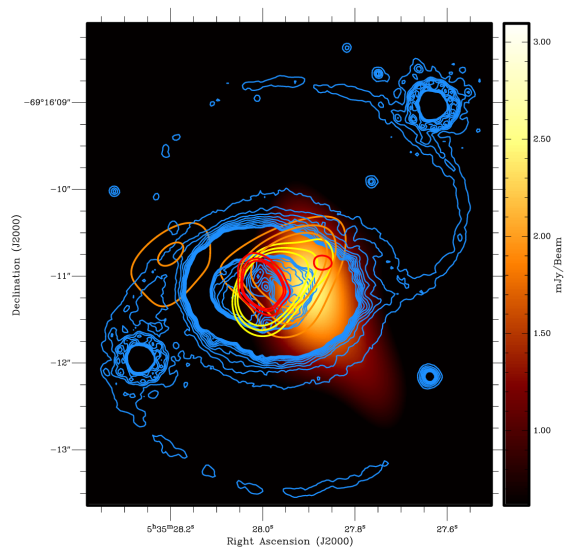
Figure 5.— Comparison of the diffraction-limited images of SNR 1987A at 102, 213 and 345 GHz, as obtained after subtraction of the scaled model flux density at 44 GHz (see Figure 1, right column), with the optical image of the remnant. In detail, the residual image at 102 GHz (brown–yellow color scale) is overlaid with the contours outlining the residual images at 213 GHz (orange) and at 345 GHz (yellow). To locate the main sites associated with dust emission, the diffraction-limited image at 672 GHz is also outlined (red) (as from Figure 1, left column). Images at 213, 345 and 672 GHz are overlaid with contours at 3, 4 and 5 $\sigma$ flux density levels. The angular beams associated with each image, as shown in Figure 1, are listed in Table 2. The HST image (lar11) is outlined via contours (blue) that highlight the structure of the outer rings, the equatorial ring and the ejecta.

3. Morphology

ALMA observations of SNR 1987A capture both the remnant emission from the ER and that from the SNR interior, where the dense ejecta sit (kam13; ind14).

While the image at 102 GHz barely resolves the two-lobe distribution of the emission, the images at 213 and 345 GHz clearly show the ringlike emission morphology, localised around the ER (see Figures  1 and 2). It is understood that the radio emission over the ER is primarily synchrotron emission, generated by the interaction of the SN shock with the dense CSM near the equatorial plane, which results in a magnetic-field discontinuity where particles are accelerated (e.g. zan10; zan13). As shown in early models of Type II SNRs (che82), the region of interaction between the SN blast and the CSM consists of a double-shock structure, with a forward shock, where ambient gas is compressed and heated, and a reverse shock, where the ejecta are decelerated. Between the two shocks, the reflected shocks, due to the forward shock colliding with the dense ER (bor97), propagate inward (zhe09; zhe10). The reverse shock at first expanded outwards, behind the forward shock, but might have been inward-moving since day $\sim 7000$. As discussed by ng13, the ring synchrotron emission is currently localised between the forward and reverse shocks, and likely has components from both the ER and high-latitude material above the equatorial plane. Truncated-shell torus models of the remnant geometry at 9 GHz indicate that the half-opening angle has been decreasing since day $\sim$7000, and is estimated at $\sim 27^{\circ}$ at day 9568 (ng13).

At 345 GHz the SNR interior is brighter, while at 672 GHz the emission is predominantly localised in the central region of the remnant. Since the emission from this region rises steeply with frequency, it has been identified with thermal dust emission (ind14), as dust grains, probably heated by ⁴⁴Ti decay and X-ray emission from the reverse shock (lar13), emit strongly in the FIR regime. The central emission, visible both in B7 and B9, appears to extend over the inner optical ejecta (see Figure 4). In particular, as noted by ind14, this inner emission shows a north–south elongation, which in B9 can be identified between PA $\sim 20^{\circ}$ and PA $\sim 30^{\circ}$, similar to that seen with HST (lar11; lar13). From both Figures 1 and 2, it can also be noticed that the SNR emission at 672 GHz includes possible emission located to the NW (see contour overlays in Figure 5). This NW feature has signal-to-noise ratio (S/N) of $3.7\,\sigma$, and integrated flux density of 6.8$\pm$0.5 mJy, i.e. $\sim$10% of the total integrated flux density at 672 GHz.

3.1. Subtracted Images

To identify the origin of the emission in the $I_{44}-$subtracted images, with respect to the structure of the remnant as seen with HST (lar11), the diffraction-limited residuals at 102, 213 and 345 GHz are superimposed in Figure 5. It can be seen that the residual at 102 GHz, characterised by $\left.{\rm S/N}\right|_{102}=6.9\,\sigma$, is mainly located on the western lobe, west of the VLBI position of SN 1987A, as determined by rey95 [RA $05^{\rm h}\;35^{\rm m}\;27\hbox{$.\!\!^{\rm s}$}968$, Dec $-69^{\circ}\;16^{\prime}\;11\hbox{$.\!\!^{\prime\prime}$}09$ (J2000)]. We note that, since the residual emission at 102 GHz has a constant flux per synthesized beam, the S/N ratio is independent on the beam size. The emission at 213 GHz (orange contours in Figure 5), with $\left.{\rm S/N}\right|_{213}=7.7\,\sigma$, peaks NW of the SN position, while fainter emission ($\left.{\rm S/N}\right|_{213}^{E}=4.2\,\sigma$) may extend NE. The residual emission at both 102 and 213 GHz is above noise levels and, thus, unlikely to be the result of image artefacts. Given the brightening of the emission from the dust in the central region of the SNR, the residual images at 345 and 672 GHz have higher S/N. In particular, at 345 GHz (yellow contours in Figure 5) $\left.{\rm S/N}\right|_{345}=17.4\,\sigma$, while, similar to the morphology at 213 GHz, the residual emission extends westwards and elongates NW, with a much fainter spot on the north-eastern section of the ER ($\left.{\rm S/N}\right|_{345}^{E}=2.4\,\sigma$). A westward-elongated morphology is present in the image at 672 GHz ($\left.{\rm S/N}\right|_{672}=12.5\,\sigma$).

The $I_{\rm B9}-$subtracted images emphasize the ringlike morphology of the synchrotron emission that mainly originates near the ER (see § 3) and, thus, the asymmetry of this emission, which is discussed in § 4. These residuals also highlight the presence of NW emission at 672 GHz, i.e. outside the inner SNR (see red contours in Figure 5). In fact, at 94, 213, and 345 GHz, it can be seen that the discontinuity in the NW sector of the ER, between PA $\sim 290^{\circ}$ and PA $\sim 300^{\circ}$, becomes more prominent after subtraction of the B9 model. Some extended emission north and NW of the ER emerges from noise at 345 GHz.

4. Asymmetry

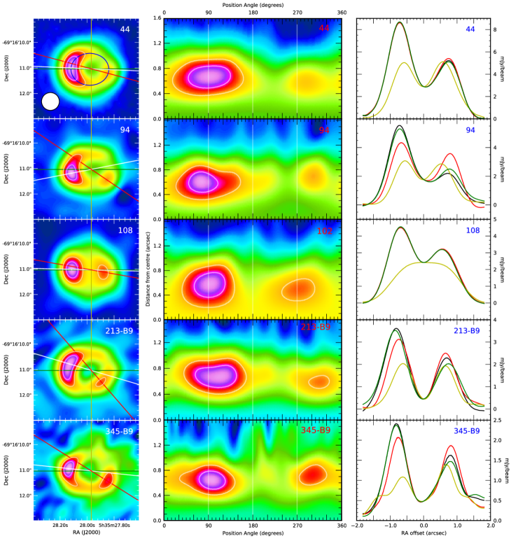
Figure 6.— Top to bottom - Left column: Stokes $I$ continuum images of SNR 1987A at 44, 94, 102, 213, and 345 GHz. The 213 (213–B9) and 345 GHz (345–B9) images are derived after subtraction of the scaled model flux density at 672 GHz (Band 9, B9). All images are resolved with a $0\hbox{$.\!\!^{\prime\prime}$}7$ circular beam (as shown in the bottom left corner of the 44 GHz image). Center column: The images on the left column are converted to polar coordinates to visualize asymmetries in the two-dimensional radial distribution. The position angle and the projected radial distance from the geometrical center of the remnant, are the new coordinates. Each image is projected along concentric ellipses (e.g. blue ellipse overlaid on the 44 GHz image). The emission intensity is conserved in the conversion. Contours at 65% and 85% levels of the emission are shown on all images (white). Right column: Radial slices through each image at four position angles (as indicated on the images on the left column), which correspond to $0^{\circ}$ (light green), $90^{\circ}$ (dark green), emission peaks on the eastern lobe (white/black) and on the western lobe (red). The radial slices are plotted against the RA offset from the VLBI position of SN 1987A as determined by rey95 [RA $05^{\rm h}\;35^{\rm m}\;27\hbox{$.\!\!^{\rm s}$}968$, Dec $-69^{\circ}\;16^{\prime}\;11\hbox{$.\!\!^{\prime\prime}$}09$ (J2000)].

The east-west asymmetry of the synchrotron emission, primarily associated with the emission morphology over the ER, is investigated from 44 to 345 GHz, as shown in Figure 6, where all images are restored with a $0\hbox{$.\!\!^{\prime\prime}$}7$ circular beam. At 213 and 345 GHz the central dust emission is subtracted, via a scaled model of the flux density as resolved in B9 (see § 2).

Considering radial sections crossing the SN site (rey95), the SNR asymmetry is firstly estimated as the ratio between the eastern peak of the radial slice crossing the maximum emission on the eastern lobe (see black/white profile in Figure 6), and the western peak of the radial slice crossing the maximum emission on the western lobe, (see red profiles in Figure 6). This ratio, $A_{p}$, emphasizes the hot spots on each side of the remnant. Alternatively, the ratio $A_{i}$ between the total flux densities integrated over the eastern and western halves of the image, is derived by splitting the image at the RA associated with the SN site. For comparison with previous asymmetry estimates (e.g. zan13), the ratio $A_{90}$ between the eastern and western peaks of the radial slice at PA $90^{\circ}$ (see dark green profile in Figure 6) is also derived. All values for $A_{p}$, $A_{i}$ and $A_{90}$, both for the images restored with a $0\hbox{$.\!\!^{\prime\prime}$}7$ circular beam (as in Figure 6) and the diffraction-limited images, are plotted in Figure  7 and listed in Table 4.

From Figure 6 it can be seen that the $A_{90}$ ratio does not fully capture the asymmetry changes with frequency, since the hot spot in the western lobe, which becomes brighter from 102 to 345 GHz, is located southwards of the 90^∘ profile. In Figure 7, the linear fits derived for both $A_{p}$ and $A_{i}$ ratios show a consistent decrease as frequencies reach the FIR. At 345 GHz, $A_{i}$ values indicate that the east-west asymmetry is reversed, thus matching the asymmetry trend seen in recent HST images (lar11), where the western side of the ring is markedly brighter. As discussed in § 3, the morphology similarities between the optical image of the SNR and the super-resolved image at 345 GHz are evident (see Figure 4).

The change of the remnant’s east-west asymmetry over time has been discussed by ng13, as the result of a progressive flattening of the shock structure in the equatorial plane, due to the shock becoming engulfed in the dense UV-optical knots in the ER, coupled with faster shocks in the east side of the remnant. While X-ray observations do not show significant difference between the NE and SW reverse shock velocities, although the NE sector is brighter (fra13), faster eastbound outer shocks have been measured in the radio (zan13) and point to an asymmetric explosion of a binary merger as SN progenitor (mor07; mor09). As the SN blast is gradually overtaking the ER, faster expanding shocks in the east would exit the ER earlier than in the west.

Table 3Asymmetry Ratios

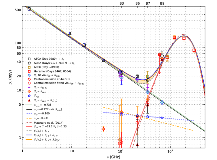
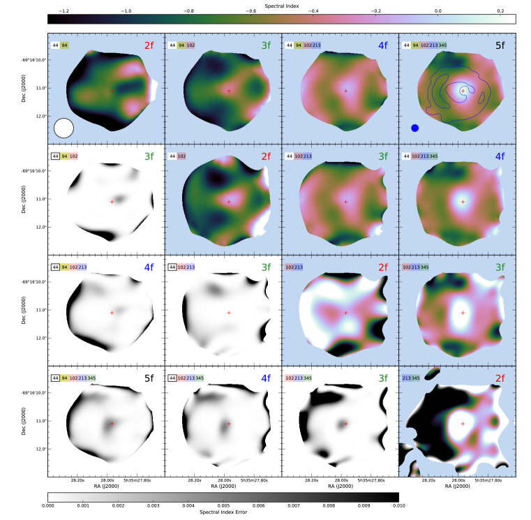
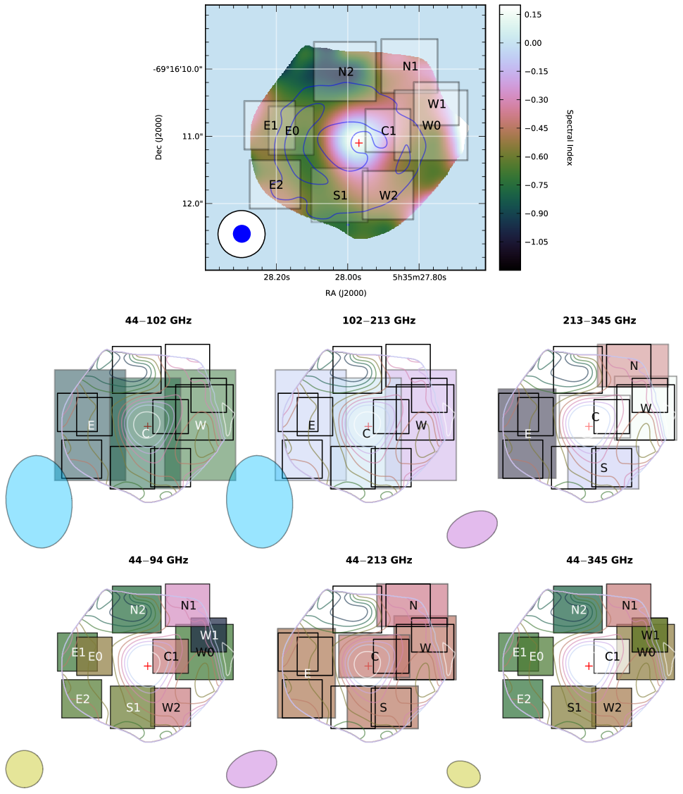
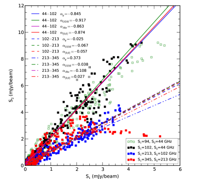
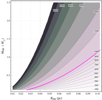
Image	$A_{p}\equiv\dfrac{S_{\nu}(E_{Max})}{S_{\nu}(W_{Max})}$		$A_{i}\equiv\left.\int\limits_{E}S_{\nu}\middle/\int\limits_{W}S_{\nu}\right.$		$A_{90}\equiv\left.S_{\nu}\left(\dfrac{E_{Max}}{W_{Max}}\right)\right|_{90^{\circ}}$
GHz	$0\hbox{$.\!\!^{\prime\prime}$}7$	DL	$0\hbox{$.\!\!^{\prime\prime}$}7$	DL	$0\hbox{$.\!\!^{\prime\prime}$}7$	DL
44	$1.61\pm 0.08$	$1.42\pm 0.05$	$1.36\pm 0.02$	$1.53\pm 0.07$	$1.69\pm 0.08$	$1.54\pm 0.05$
94	$1.55\pm 0.05$	$\cdots$	$1.18\pm 0.04$	$\cdots$	$1.88\pm 0.07$	$\cdots$
102	$1.44\pm 0.04$	$\cdots$	$1.10\pm 0.04$	$\cdots$	$1.40\pm 0.07$	$\cdots$
213	$1.28\pm 0.03$	$1.43\pm 0.05$	$1.24\pm 0.06$	$1.23\pm 0.02$	$1.43\pm 0.02$	$1.49\pm 0.05$
213$-I_{\rm B9}$	$1.44\pm 0.03$	$\cdots$	$1.30\pm 0.02$	$\cdots$	$1.19\pm 0.03$	$\cdots$
345	$\cdots$	$1.28\pm 0.03$	$\cdots$	$0.78\pm 0.04$	$\cdots$	$1.16\pm 0.03$
345$-I_{\rm B9}$	$1.30\pm 0.02$	$\cdots$	$0.80\pm 0.02$	$\cdots$	$1.48\pm 0.04$	$\cdots$
The effects of the asymmetric shock propagation are likely to emerge in the transition from radio to FIR rather than at lower frequencies, due to the shorter synchrotron lifetime at higher frequencies. To estimate the synchrotron lifetime in the FIR range, we use the approximation that, in a magnetic field of strength $B$, all the radiation of an electron of energy $E$ is emitted only at the critical frequency $\nu_{c}$ (ryb79). Considering the electron s orbit is inclined at a pitch angle $\theta$ to the magnetic field, the synchrotron lifetime, $\tau_{e}$, can be derived as a function of $\nu_{c}$ (e.g. con92) $$\tau_{e}\equiv{E\over|dE/dt|}\sim 1.06\times 10^{9}(B\,{\rm sin}\theta)^{-3/2}\nu_{c}^{-1/2},$$ (1) where $\tau_{e}$ is expressed in years, $B$ in $\mu$G and $\nu$ in GHz. As the electrons are expected to have an isotropic distribution of pitch angles, $\langle{\rm sin}^{2}\theta\rangle=2/3$; for $200\lesssim\nu\lesssim 400$ GHz, and assuming a magnetic field strength at the shock front of $10\lesssim B\lesssim 20$ mG (ber06; ber11), in the radio/FIR transition we can estimate $20\lesssim\tau_{e}\lesssim 80$ yr. However, since it is likely that sub-diffusive particle transport (kir96) is taking place in regions of the SNR, in conjunction with efficient CR acceleration (glu13), local magnetic-field amplifications could exceed the above limits by at least an order of magnitude (bel01). In this scenario, the local $\tau_{e}$ would be of the order of months. Therefore, with regions in the remnant where electrons might be unable to cross the emission sites within their radiative life-time, the synchrotron emission at FIR frequencies would require the presence of relatively fresh injected and/or re-accelerated electrons to match the emission distribution at lower frequencies.
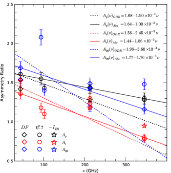
Figure 7.— Asymmetry ratios of Stokes $I$ images of SNR 1987A from 44 to 345 GHz. With reference to Table 4, the east-west asymmetry ratios estimated via three different methods are indicated as: $A_{p}$ (black symbols); $A_{i}$ (red symbols); $A_{90}$ (blue symbols). Asymmetry ratios are derived from the diffraction-limited images (diamonds) (see Figure 1), from the images restored with a $0\hbox{$.\!\!^{\prime\prime}$}7$ circular beam (circles) (see Figure 6); and from images obtained after the subtraction of the dust emission component (stars) (see Figure 6). Tentative linear fits are shown for $A_{p}$ (black fits), $A_{i}$ (red fits) and $A_{90}$ (blue fits), based on all ratios derived via each method. The orthogonal distance regression ($A_{ODR}$) and the robust fitting from the square root of absolute residuals ($A_{Abs}$), are tested for linear interpolation. The combined fits for the $A_{p}$ and $A_{i}$ ratios yield an average $A(\nu)\sim A(\nu_{0})-1.9\pm 0.8\times 10^{-3}\nu$, where $\nu$ is expressed in GHz and $A(\nu_{0}=30)=1.57\pm 0.13$. 5. Spectral Energy Distribution The spectral energy distribution for ATCA data from 1.4 to 94 GHz and ALMA data is shown in Figure 8. To match the average epoch of the ALMA data, the ATCA data are scaled to day 9280, via exponential fitting parameters derived for ATCA flux densities from day 8000, as measured at 1.4, 8.6 and 9 GHz (Zanardo et al., in preparation; sta14). Across the transition from radio to FIR frequencies, the observed spectrum consists of the sum of thermal and non-thermal components. As described in § 2, to identify the dust component of the emission from the inner regions of the remnant, the B9 model flux density, $S_{\rm B9}$, has been scaled to fit the emission measured in the SNR central region at 94–345 GHz ($S_{\rm B9_{\rm\,fit}}$, hollow red circles in Figure 8). The subtraction of $S_{\rm B9_{\rm\,fit}}$ from the visibilities at 94–345 GHz yields the residual flux densities indicated as $S_{\nu}-S_{\rm B9_{\rm\,fit}}$ (purple bars in Figure 8), as for the images shown in the central column of Figure 1. The flux densities $S_{\rm B9_{\rm\,fit}}$ derived in B6 and B7, together with the total integrated flux density measured in B9 ($S_{\rm B9}$), although obtained via a different reduction technique, have been associated by ind14 with dust grains, in conjunction with data from Herschel (mat11) and the Atacama Pathfinder Experiment (APEX; lak12b) (see Figure 8). Similarly (see § 2), to separate the non-thermal emission from that thermal, the 44 GHz model flux density, $S_{44}$, has been scaled to fit the toroidal component of the emission at 94–672 GHz (blue/cyan diamonds in Figure 8). By fitting the resulting $S_{44_{\rm\,fit}}$ components and the ATCA flux densities at 1.4–44 GHz, we obtain, at day 9280, the synchrotron spectral index $\alpha_{s}=-0.727\pm 0.020$, with $S_{\nu}(\alpha_{s})\propto\nu^{\alpha_{s}}$. The spectral index measured from 1.4 to 94 GHz, i.e. for ATCA data only, is $\alpha_{{}_{\rm ATCA}}=-0.735\pm 0.028$. While $\alpha_{s}$ is slightly flatter than $\alpha_{{}_{\rm ATCA}}$, both values are consistent with the progressive flattening of the radio spectrum measured since day $\sim 5000$ (zan10). The subtraction of $S_{44_{\rm\,fit}}$ from the visibilities at 94–672 GHz, gives the residual flux densities $S_{\nu}-S_{44_{\rm\,fit}}$ (red/orange diamonds in Figure 8), as for the images shown in the right column of Figures 1. In B3, B6 and B7, $S_{\nu}-S_{44_{\rm\,fit}}>S_{\rm B9_{\rm\,fit}}$, i.e. the residuals exceed the emission expected from the dust. While the subtraction of the flux densities is inevitably affected by errors (see Table 2), given that the $I_{44}-$subtracted images have a S/N$\,\gtrsim 7\,\sigma$ and the residual emission appears primarily located westwards of the optical ejecta (see § 3.1), we investigate the nature of this emission excess as: (1) free-free emission from an ionized fraction of the inner ejecta; (2) synchrotron emission from a compact source located in the inner regions of the remnant; (3) emission from grains of very cold dust. Figure 8.— Spectral energy distribution (SED) of SNR 1987A from radio to FIR, with data from: ATCA at 1.4 GHz (Zanardo et al. in prep), 9 GHz (ng13), 18 and 44 GHz (zan13), and 94 GHz (lak12); ALMA at 102 GHz (Band 3, B3), 213 GHz (Band 6, B6), 345 GHz (Band 7, B7) and 672 GHz (Band 9, B9) (this paper); the Atacama Pathfinder EXperiment (APEX) at 345 and 857 GHz (lak12b); the Herschel Space Observatory at 600 – 3000 GHz (mat11). The brown dash-dot-dotted curve is the amorphous carbon dust fit for ALMA data and Herschel observations carried out in 2012 (mat14, submitted). To match the average epoch of ALMA observations, ATCA data are scaled to day 9280, via exponential fitting parameters derived for ATCA flux densities from day 8000, as measured at 1.4, 8.6 and 9 GHz (Zanardo et al., in preparation; sta14). The hollow red diamond indicates the central emission measured at 44 GHz as reported by zan13, scaled to day 9280. The difference between possible spectral fits is highlighted in light orange. See § 5 for a detailed description of this figure. 5.1. Free-Free Emission To estimate the free-free radiation in the SNR as imaged with ALMA, we hypothesize an ionized portion of the ejecta as an approximately spherical region, located inside the ER. Using the beam size of the super-resolved $I_{44}-$subtracted image at 102 GHz as an upper limit, we consider the radius of the spherical region up to $R_{s}\sim 0\hbox{$.\!\!^{\prime\prime}$}40$ ($\approx 3.08\times 10^{17}$ cm). Such radius covers the extent of the inner ejecta as imaged in the optical (lar13), and stretches to the likely radius of the reverse shock, qualitatively identified with the inner edge of the emission over the ER (see Figure 4). Given that the pre-supernova mass has been estimated between $14\,M_{\sun}$ and $20\,M_{\sun}$ (sma09), if we assume that the Hii region in the ejecta has a uniform density $\rho_{ej}(r)=3\,M_{\rm HII}(4\pi r^{3})^{-1}$, we set $0.7\,M_{\sun}\lesssim M_{\rm HII}\lesssim 2.5\,M_{\sun}$. The lower limit, $M_{\rm HII}\sim 0.7\,M_{\sun}$, i.e. $\rho_{ej}(r=R_{s})=1.1\times 10^{-20}$, represents a partial ionization of the ejecta by X-ray flux, either within the inner region or on the outer layer. The upper limit, $M_{\rm HII}\sim 2.5\,M_{\sun}$, i.e. $\rho_{ej}(r=R_{s})=4.1\times 10^{-20}$ g cm-3 matches the density model by bli00 scaled to the current epoch (see Figure 21 in fra13), and corresponds to complete ionization of the H and He mass within $R_{s}$. The optical depth associated with the Hii region along the line of sight (los) can be estimated as $$\tau_{ff}\approx 3.28\times 10^{-7}\,T_{4}^{-1.35}\nu^{-2.1}N_{e}^{2}R_{s},$$ (2) where $T_{4}=T_{e}/{\rm(10^{4}\,K)}$, $\nu$ is in GHz, $N_{e}$ is in cm-3 and $R_{s}\approx\int_{\rm los}\mathrm{d}l$ is in pc. For $T_{4}\sim 1$, given the emission measure $4.6\times 10^{6}\lesssim{\rm EM}\lesssim 5.9\times 10^{7}$ cm-6 pc, where ${\rm EM}=N_{e}^{2}R_{s}$, at frequencies $102\lesssim\nu\lesssim 672$ GHz the emission becomes nearly transparent as $2.28\times 10^{-6}\lesssim\tau_{ff}\lesssim 1.2\times 10^{-3}$. The flux associated with the ionized component of the ejecta, can then be derived as $$S_{\nu_{ff}}\propto\tau_{ff}(\nu){2kT\over\lambda^{2}}\Omega\propto\nu^{-0.1}.$$ (3) Considering the solid angle $\Omega$ subtended by the same radius, $R_{s}$, at all frequencies, for the lower limit $M_{\rm HII}\approx 0.7\,M_{\sun}$, i.e. $N_{e}=6.8\times 10^{3}$ cm-3, $S_{\nu_{ff}}\sim(S_{\nu}-S_{44_{\rm\,fit}})$ at 102 and 213 GHz, as Eq. 3 yields $S_{102_{ff}}\sim 3.9$ mJy, $S_{213_{ff}}\sim 3.2$ mJy, $S_{345_{ff}}\sim 3.1$ mJy and $S_{672_{ff}}\sim 2.9$ mJy. These $S_{\nu_{ff}}$ values (blue stars in in Figure 8) would well fit the SED (see blue fit in Figure 8). If the Hii density is considerably higher, as given by the upper limit $M_{\rm HII}\approx 2.5\,M_{\sun}$, the derived $S_{\nu_{ff}}$ fluxes would exceed the emission residuals by an order of magnitude. As a constraint to the free-free emission component, the hypothesized Hii region would also produce optical and near-IR Hi recombination lines. The resultant H${\alpha}$ flux can be estimated as $$S_{\rm H\alpha}\approx\epsilon\,N_{e}N_{+}\,\biggl{(}{{4}\over{3}}\pi R_{s}^{3}\biggr{)}{{f}\over{4\pi d^{2}}},$$ (4) where $\epsilon\propto\alpha_{A}$ is the emissivity of the H$\alpha$ line per unit volume, with $\alpha_{A}=\alpha_{A}(T)={\sum_{n}\alpha_{n}(T)}$ the total recombination coefficient, $f$ is the volume filling factor and $d$ is the distance to the source. If one adopts $\epsilon\approx 3.53\times 10^{-25}\,T_{4}^{-0.92}$ erg cm-3 s-1 for $T_{4}\simeq 0.5$ (e.g. sto95), the number of ions $N_{+}=N_{e}=6.8\times 10^{3}$ cm-3 as for the lower limit assumed for the density of the Hii region, and $R_{s}\approx 3.08\times 10^{17}$ cm, for $f\sim 1$ one obtains $S_{\rm H\alpha}\approx 1.26\times 10^{-11}$ erg cm2 s-1. To match the H$\alpha$ flux from the core measured by fra13 (see Figure 8 therein) at $\sim 1.4\times 10^{-14}$ erg cm2 s-1 on day 9000, the estimated $S_{\rm H\alpha}$ would have to undergo $7.4$ magnitudes of extinction. Such extinction is possible but improbable. We note that the above $S_{{\rm H}\alpha}$ also exceeds the H$\alpha$ emission by the reverse shock, measured at $\sim 2.0\times 10^{-13}$ erg cm2 s-1 on day 9000, and associated with a density $250\lesssim N_{+}\lesssim 750$ cm-3 (fra13). As regards the magnitude of the flux from the Br-$\gamma$ line, the model estimate by kja10 on day 6840 is a factor of $\sim 10^{-2}$ smaller than the $S_{\rm H\alpha}$ derived from Eq. 4, while this is mainly associated with emission from the hot spots in the ER. In the absence of external X-ray heating, both the heating and ionization would be powered by radioactive decays in the core. The resultant flux, estimated via models as in koz98, would be several orders of magnitude smaller than the lower limit for $S_{\nu_{ff}}$. Another possible source of ionizing emission is a pulsar wind nebula (PWN) in the SNR interior. The properties of any PWN are very uncertain (see § 7), but there is the expectation that line emission would accompany free-free emission also in this case. 5.2. Flat-Spectrum Synchrotron Emission A flat spectral index could also be attributed to a second synchrotron component. As shown in Figure 8, within $102\leq\nu\leq 672$ GHz, a synchrotron component with spectral index $\alpha_{p}=-0.231$ fits the residuals ($S_{\nu}-S_{44_{\rm\,fit}}$) at 102 and 213 GHz. Synchrotron emission with $-0.4\lesssim\alpha\lesssim-0.1$ fits the spectrum in the radio/FIR transition and could originate from a compact source near the center of the SNR. In the case of a central pulsar, the synchrotron emission would be generated by the shocked magnetized particle wind (gae06). The scenario of a synchrotron-emitting PWN in the inner SNR is explored in § 7. 5.3. Dust Emission If the excess emission is due to an additional synchrotron component, $S_{\nu}(\alpha_{p})\propto\nu^{-0.2}$, this would provide a constraint to the net dust emission, $S_{\nu_{d}}$, in ALMA data. The subtraction $S_{\nu}-S_{44_{\rm\,fit}}-S_{\nu}(\alpha_{p})$, where $S_{\nu_{p}}=S_{0_{p}}(\nu/\nu_{0})^{\alpha_{p}}$ with $S_{0_{p}}=3.5\pm 3.1$ mJy as from Table 2, leads to $S_{213_{d}}\sim 0.7$ mJy, $S_{345_{d}}\sim 4.9$ mJy and $S_{672_{d}}\sim 45.0$ mJy (black triangles in Figure 8). We note that $S_{672_{d}}$ coincides with the integrated flux density of the central feature of the related image, which extends over the inner ejecta as seen with HST (see Figure 4). The net dust can be fitted via a modified Planck curve of thermal emission, as $$S_{\nu_{d}}(\beta,T)={M_{\rm dust}\over d^{2}}\,\kappa_{\nu}\,B_{\nu}(T)\propto\nu^{\,\beta}\,B_{\nu}(T),$$ (5) where $M_{\rm dust}$ is the dust mass, $\kappa_{\nu}=3\,Q_{\nu}/4\rho\,a_{\nu}$ is the dust mass absorption coefficient, with $Q_{\nu}$ the absorption efficiency for spherical grains of density $\rho$ and radius $a_{\nu}$, $1\lesssim\beta\lesssim 2$ for insterstellar dust (e.g. cor14 and references therein) and $B_{\nu}(T)$ is the Planck function. As shown in Figure 8, the best fit of both ALMA fluxes, as reported in this paper, and Herschel fluxes, as from mat11, yields $\beta=1.23$ and dust temperature $T=22.2$ K. The thermal peak of the SED has been previously fitted (mat11; lak11; lak12; lak12b) with temperatures estimated between 17 and 26 K, while ind14 fit amorphous carbon dust at $T=26\pm 3$ K. The sum of the main synchrotron component, $S_{\nu}\propto\nu^{-0.73}$, and the emission component from dust grains at $T\sim 22$ K is lower than the measured ALMA flux densities at 213 and 345 GHz (see dashed gray fit in Figure 8). To match the emission excess of $\sim 3$ mJy in this frequency range, we could also postulate a second dust component. This would require very cold dust at $T\lesssim 5$ K, i.e. at temperatures where the assumption of either amorphous carbon or silicates leads to dust masses implausibly large for physically realistic grains. In particular, as from Eq. 5, at 345 GHz a flux density of $\sim 3$ mJy would require dust at $T\sim 3$ K with $M_{\rm dust}\sim 50\,M_{\sun}$, as obtained by using $k_{\nu}\sim 2.5$ cm2 g-1 for amorphous carbon (zub96; zub04). We note that warmer dust at $T\sim$ 180 K has been identified by dwe10 in the ER, where the dust grains are likely collisionally heated by the expanding radiative shocks (bou06).
6. Spectral Index Variations Figure 9.— In color scale are maps of the spectral index distribution in SNR 1987A, as derived from images at 44, 94, 102, 213, and 345 GHz. The source images are reduced with identical procedure and restored with a circular beam of $0\hbox{$.\!\!^{\prime\prime}$}8$. To match the average epoch of ALMA observations, ATCA data at 44 and 94 GHz are scaled to day 9280, via exponential fitting parameters derived for ATCA flux densities from day 8000, as measured at 8.6 and 9 GHz (Zanardo et al., in preparation). The spectral maps are derived from flux densities at 2, 3, 4, and 5 frequencies, and labelled as 2f, 3f, 4f, and 5f, respectively (top right corner). The frequencies used in each map are indicated, in GHz, on the top left corner. Image regions below the highest rms noise level are masked. The upper limit of the spectral index color scale is set to $\alpha=0.25$, therefore map regions with spectral indices greater than 0.25 appear in white. In grey scale are maps of the error associated with $\alpha$ in the power-law fit, $S_{\nu}\sim\nu^{\alpha}$, used for spectral maps of flux densities at 3, 4, and 5 different frequencies, and labelled as 3f, 4f, and 5f, respectively. To emphasize the error distribution, while using a linear gradient of the grey color scale, map regions with errors greater that 0.01 appear in black. In the top right map, the contours of the 44 GHz image, resolved with a $0\hbox{$.\!\!^{\prime\prime}$}25$ circular beam, are shown at the $15\%$ and $60\%$ emission levels (in blue). The red cross indicates the VLBI position of SN 1987A as determined by rey95 [RA $05^{\rm h}\;35^{\rm m}\;27\hbox{$.\!\!^{\rm s}$}968$, Dec $-69^{\circ}\;16^{\prime}\;11\hbox{$.\!\!^{\prime\prime}$}09$ (J2000)]. Figure 10.— Top $-$ Four-frequency (44–94–213–345 GHz) spectral index intensity map with an angular resolution of $0\hbox{$.\!\!^{\prime\prime}$}8$, where ATCA data at 44 and 94 GHz are scaled to day 9280. The map is superimposed with the contours of the 44 GHz image, resolved with a $0\hbox{$.\!\!^{\prime\prime}$}25$ circular beam, at the $15\%$ and $60\%$ emission levels (in blue). The regions used to derive the spectral indices $\alpha_{TT}$, via T-T plots, are indicated by grey/white squares. Bottom $-$ The T-T plots are applied to 6 pairs of frequencies: $44-102$ GHz, $102-213$ GHz, $213-345$ GHz, $44-94$ GHz, $44-213$ GHz, and $44-345$ GHz. The controlling beam associated with each pair of frequencies is shown on the lower left corner of the images. The T-T boxes are color-coded according to the resultant $\alpha_{TT}$ value. For image pairs of angular resolution lower than $0\hbox{$.\!\!^{\prime\prime}$}8$, larger T-T boxes are used as outlined. All T-T boxes are drawn on top of the 4-frequency spectral map, highlighted by contours spaced at $\Delta\alpha=0.1$, which are colored according to the associated spectral index. The red cross indicates the VLBI position of SN 1987A as determined by rey95. The $\alpha_{TT}$ values resulting from the six frequency pairs are detailed in Table 4. Table 4Regional Spectral Indices $\alpha_{TT}(S_{1},S_{2})$ $\alpha_{M_{\mu}}(S_{1,2,3,4})$ Region Fit (44,102) (102,213) (213,345) (44,94) (44,213) (44,345) (44,94,213,345) N y  $\cdots$  $\cdots$ $-0.33\pm 0.02$  $\cdots$ $-0.38\pm 0.03$  $\cdots$  $\cdots$ ODR  $\cdots$  $\cdots$ $-0.41\pm 0.02$  $\cdots$  $\cdots$  $\cdots$  $\cdots$ Abs  $\cdots$  $\cdots$ $-0.40\pm 0.02$  $\cdots$ $-0.37\pm 0.03$  $\cdots$  $\cdots$ (0,0)  $\cdots$  $\cdots$ $-0.05\pm 0.04$  $\cdots$ $-0.43\pm 0.05$  $\cdots$  $\cdots$ N1 y  $\cdots$  $\cdots$  $\cdots$ $-0.28\pm 0.08$  $\cdots$ $-0.39\pm 0.02$ $-0.39\pm 0.09$ ODR  $\cdots$  $\cdots$  $\cdots$ $-0.31\pm 0.09$  $\cdots$ $-0.42\pm 0.02$  $\cdots$ Abs  $\cdots$  $\cdots$  $\cdots$ $-0.27\pm 0.08$  $\cdots$ $-0.35\pm 0.03$  $\cdots$ (0,0)  $\cdots$  $\cdots$  $\cdots$ $-0.36\pm 0.14$  $\cdots$ $-0.40\pm 0.04$  $\cdots$ N2 y  $\cdots$  $\cdots$  $\cdots$ $-0.73\pm 0.03$  $\cdots$ $-0.81\pm 0.08$ $-0.85\pm 0.14$ ODR  $\cdots$  $\cdots$  $\cdots$ $-0.76\pm 0.03$  $\cdots$  $\cdots$  $\cdots$ Abs  $\cdots$  $\cdots$  $\cdots$ $-0.77\pm 0.03$  $\cdots$  $\cdots$  $\cdots$ (0,0)  $\cdots$  $\cdots$  $\cdots$ $-0.84\pm 0.04$  $\cdots$ $-0.89\pm 0.07$  $\cdots$ E y $-0.95\pm 0.02$ $-0.07\pm 0.02$ $-1.05\pm 0.04$  $\cdots$ $-0.48\pm 0.02$  $\cdots$  $\cdots$ ODR $-0.95\pm 0.01$ $-0.07\pm 0.03$  $\cdots$  $\cdots$ $-0.60\pm 0.05$  $\cdots$  $\cdots$ Abs $-0.95\pm 0.02$ $-0.06\pm 0.03$ $-1.12\pm 0.04$  $\cdots$ $-0.47\pm 0.02$  $\cdots$  $\cdots$ (0,0) $-0.97\pm 0.02$ $-0.03\pm 0.03$ $0.11\pm 0.07$  $\cdots$ $-0.46\pm 0.02$  $\cdots$  $\cdots$ E0 y  $\cdots$  $\cdots$  $\cdots$ $-0.55\pm 0.03$  $\cdots$ $-0.68\pm 0.03$ $-0.60\pm 0.03$ ODR  $\cdots$  $\cdots$  $\cdots$ $-0.59\pm 0.03$  $\cdots$ $-0.72\pm 0.04$  $\cdots$ Abs  $\cdots$  $\cdots$  $\cdots$ $-0.54\pm 0.03$  $\cdots$ $-0.66\pm 0.03$  $\cdots$ (0,0)  $\cdots$  $\cdots$  $\cdots$ $-0.69\pm 0.07$  $\cdots$ $-0.71\pm 0.06$  $\cdots$ E1 y  $\cdots$  $\cdots$  $\cdots$ $-0.65\pm 0.04$  $\cdots$ $-0.66\pm 0.04$ $-0.52\pm 0.13$ ODR  $\cdots$  $\cdots$  $\cdots$ $-0.68\pm 0.04$  $\cdots$ $-0.68\pm 0.04$  $\cdots$ Abs  $\cdots$  $\cdots$  $\cdots$ $-0.70\pm 0.05$  $\cdots$ $-0.65\pm 0.04$  $\cdots$ (0,0)  $\cdots$  $\cdots$  $\cdots$ $-0.78\pm 0.08$  $\cdots$ $-0.68\pm 0.04$  $\cdots$ E2 y  $\cdots$  $\cdots$  $\cdots$ $-0.60\pm 0.03$  $\cdots$ $-0.73\pm 0.03$ $-0.55\pm 0.12$ ODR  $\cdots$  $\cdots$  $\cdots$ $-0.63\pm 0.03$  $\cdots$ $-0.74\pm 0.02$  $\cdots$ Abs  $\cdots$  $\cdots$  $\cdots$ $-0.65\pm 0.03$  $\cdots$ $-0.72\pm 0.03$  $\cdots$ (0,0)  $\cdots$  $\cdots$  $\cdots$ $-0.74\pm 0.04$  $\cdots$ $-0.73\pm 0.03$  $\cdots$ S y  $\cdots$  $\cdots$ $-0.05\pm 0.05$  $\cdots$ $-0.45\pm 0.02$  $\cdots$  $\cdots$ ODR  $\cdots$  $\cdots$ $-0.10\pm 0.04$  $\cdots$  $\cdots$  $\cdots$  $\cdots$ Abs  $\cdots$  $\cdots$ $-0.23\pm 0.03$  $\cdots$ $-0.44\pm 0.02$  $\cdots$  $\cdots$ (0,0)  $\cdots$  $\cdots$ $-0.22\pm 0.03$  $\cdots$ $-0.53\pm 0.07$  $\cdots$  $\cdots$ S1 y  $\cdots$  $\cdots$  $\cdots$ $-0.61\pm 0.02$  $\cdots$ $-0.52\pm 0.07$ $-0.63\pm 0.07$ ODR  $\cdots$  $\cdots$  $\cdots$  $\cdots$  $\cdots$  $\cdots$  $\cdots$ Abs  $\cdots$  $\cdots$  $\cdots$ $-0.60\pm 0.02$  $\cdots$ $-0.56\pm 0.07$  $\cdots$ (0,0)  $\cdots$  $\cdots$  $\cdots$ $-0.95\pm 0.18$  $\cdots$ $-0.67\pm 0.09$  $\cdots$ W y $-0.77\pm 0.02$ $-0.11\pm 0.03$ $0.25\pm 0.04$  $\cdots$ $-0.40\pm 0.06$  $\cdots$  $\cdots$ ODR $-0.78\pm 0.02$ $-0.11\pm 0.02$ $0.17\pm 0.02$  $\cdots$ $-0.43\pm 0.06$  $\cdots$  $\cdots$ Abs $-0.77\pm 0.02$ $-0.10\pm 0.03$ $0.08\pm 0.04$  $\cdots$ $-0.43\pm 0.06$  $\cdots$  $\cdots$ (0,0) $-0.76\pm 0.02$ $-0.18\pm 0.03$ $0.16\pm 0.03$  $\cdots$ $-0.49\pm 0.05$  $\cdots$  $\cdots$ W0 y  $\cdots$  $\cdots$  $\cdots$ $-0.69\pm 0.03$  $\cdots$ $-0.49\pm 0.09$ $-0.53\pm 0.05$ ODR  $\cdots$  $\cdots$  $\cdots$ $-0.77\pm 0.04$  $\cdots$ $-0.57\pm 0.10$  $\cdots$ Abs  $\cdots$  $\cdots$  $\cdots$  $\cdots$  $\cdots$ $-0.54\pm 0.10$  $\cdots$ (0,0)  $\cdots$  $\cdots$  $\cdots$ $-0.66\pm 0.03$  $\cdots$ $-0.49\pm 0.11$  $\cdots$ W1 y  $\cdots$  $\cdots$  $\cdots$ $-0.93\pm 0.09$  $\cdots$ $-0.61\pm 0.09$ $-0.37\pm 0.11$ ODR  $\cdots$  $\cdots$  $\cdots$ $-0.97\pm 0.08$  $\cdots$  $\cdots$  $\cdots$ Abs  $\cdots$  $\cdots$  $\cdots$ $-0.99\pm 0.08$  $\cdots$ $-0.60\pm 0.09$  $\cdots$ (0,0)  $\cdots$  $\cdots$  $\cdots$ $-0.75\pm 0.10$  $\cdots$ $-0.51\pm 0.15$  $\cdots$ W2 y  $\cdots$  $\cdots$  $\cdots$ $-0.40\pm 0.11$  $\cdots$ $-0.50\pm 0.02$ $-0.47\pm 0.11$ ODR  $\cdots$  $\cdots$  $\cdots$ $-0.44\pm 0.11$  $\cdots$ $-0.52\pm 0.02$  $\cdots$ Abs  $\cdots$  $\cdots$  $\cdots$ $-0.35\pm 0.12$  $\cdots$ $-0.49\pm 0.02$  $\cdots$ (0,0)  $\cdots$  $\cdots$  $\cdots$ $-0.52\pm 0.14$  $\cdots$ $-0.51\pm 0.02$  $\cdots$ C y $-0.86\pm 0.08$ $-0.00\pm 0.04$ $1.20\pm 0.04$  $\cdots$ $-0.43\pm 0.02$  $\cdots$  $\cdots$ ODR $-0.90\pm 0.08$ $-0.00\pm 0.03$ $1.97\pm 0.09$  $\cdots$  $\cdots$  $\cdots$  $\cdots$ Abs $-0.86\pm 0.08$ $-0.00\pm 0.03$ $2.25\pm 0.11$  $\cdots$ $-0.44\pm 0.01$  $\cdots$  $\cdots$ (0,0) $-0.84\pm 0.08$ $-0.09\pm 0.04$  $\cdots$  $\cdots$ $-0.43\pm 0.02$  $\cdots$  $\cdots$ C1 y  $\cdots$  $\cdots$  $\cdots$ $-0.40\pm 0.08$  $\cdots$  $\cdots$ $-0.01\pm 0.06$ ODR  $\cdots$  $\cdots$  $\cdots$  $\cdots$  $\cdots$  $\cdots$  $\cdots$ Abs  $\cdots$  $\cdots$  $\cdots$ $-0.47\pm 0.08$  $\cdots$  $\cdots$  $\cdots$ (0,0)  $\cdots$  $\cdots$  $\cdots$ $-0.73\pm 0.15$  $\cdots$  $\cdots$  $\cdots$ Figure 11.— Temperature-temperature (T-T) plot of the whole SNR, where flux densities ($S_{1}$ vs $S_{2}$) are plotted instead of brightness temperatures. Four frequency pairs are included: 44–94 GHz (green hollow squares); 44–102 GHz (solid black squares); 102–213 GHz (solid blue squares); 213–314 GHz (solid red squares). Data points for the 44–94 GHz frequency pair are not fitted. The given spectral indices are derived from different linear interpolations: least-square fit from vertical squared errors, $\alpha_{y}$ (blue); orthogonal distance regression, $\alpha_{ODR}$ (green); robust fitting from the square root of absolute residuals, $\alpha_{Abs}$ (magenta); linear regression with forced zero interception $(S_{1}=0,S_{2}=0)$, $\alpha_{(0,0)}$ (red). The spectral index distribution across the remnant is investigated via multi-frequency spectral index maps and the T-T plot method (cos60; tur62). Spectral index maps are derived from images at 44, 94, 102, 213 and 345 GHz. In Figure 9, the maps resulting from the combination of images at two, three, four and five frequencies are shown. All images are reduced with identical procedure and restored with a circular beam of $0\hbox{$.\!\!^{\prime\prime}$}8$. ATCA data at 44 and 94 GHz are scaled to day 9280, via exponential fitting parameters derived for ATCA flux densities from day 8000, as measured at 8.6 and 9 GHz (Zanardo et al., in preparation). While the two-frequency maps are derived from direct division of the flux densities, the maps derived from 3, 4 and 5 frequencies are more accurate, as the solution minimizes the function $${\boldsymbol{\varepsilon}}_{pq}={\sum_{k=1}^{n}}\,{\left\lvert\,S_{\nu_{k}}^{{}^{\,pq}}(\alpha_{M}^{{}^{pq}})-S_{\nu_{0}}^{{}^{\,pq}}\biggl{(}{\nu_{k}\over\nu_{0}}\biggr{)}^{\alpha_{M}^{{}^{pq}}}\right\rvert}^{2}$$ (6) at each pixel of coordinates $(p,q)$, for images at $\nu_{k}$ frequencies, with $n\geq 3$. In Figure 9, it can be seen that the spectral indices overall become flatter as the frequencies reach the FIR. For all maps, the spectral index, $\alpha_{M}$, varies between $-1.25$ and $0.25$, while in the $5-$frequency map the index range narrows to $-0.96\leq\alpha_{M}\leq 0.18$. In most of the multi-frequency maps, $\alpha_{M}$ is steeper on the eastern half of the SNR, while flat spectral indices surround the center, where the bulk of dust sits (see § 3), and extend onto the NW and SW regions of the remnant. With reference to the $5-$frequency map, $-0.9\lesssim\alpha_{M}\lesssim-0.6$ on the eastern lobe and $-0.4\lesssim\alpha_{M}\lesssim 0$ on the western side of the SNR, with $\alpha_{M}\sim 0$ around the central region and $-0.4\lesssim\alpha_{M}\lesssim-0.3$ predominantly in the NW quadrant (PA $\sim 330^{\circ}$) and in the SW quadrant (PA $\sim 210^{\circ}$). The T-T plot method is applied to two images at different frequencies, each obtained with identical reduction process and with the same angular resolution. The spectral variations are assessed over image regions not smaller than the beam size, where the spectral index, $\alpha_{TT}$ , is determined from the flux density slope $m$, where $S_{2}=m\,S_{1}+q$. The regions used for the T-T plots are shown in Figure 10. Six frequency pairs are considered: 44$-$102 GHz, 102$-$213 GHz, 213$-$345 GHz; and 44$-$94 GHz, 44$-$213 GHz and 44$-$345 GHz. Different box sizes are used to suit the controlling beam of each frequency pair. All derived $\alpha_{TT}$ values are listed in Table 4. Similarly to the trend of $\alpha_{M}$, $\alpha_{TT}$ values become flatter at higher frequencies (see Figure 11). From 102 to 213 GHz, $\alpha_{TT}\approx-0.1$ across the whole remnant (see Figure 10), while from 213 to 345 GHz the spectral distribution appears markedly split in two larger regions (see also the two-frequency map in Figure 9), with very flat indices on the western half of the SNR and steep indices on the eastern side. For the frequency pairs 102–213 and 213–345 GHz, the T-T plots for the eastern region (see E in Table 4) give $\Delta\alpha_{TT}=\alpha_{(102,\,213)}-\alpha_{(213,\,345)}=1.0\pm 0.07$. This could be indication of a local spectral break at 213 GHz. Using $\nu_{c}=213$ GHz in Eq. 1, for $B=20$ mG, $\tau_{e}\sim 35$ yr. However, given the high Mach number ($\mathcal{M}\sim 10^{4}$) of the eastbound shocks (zan13), likely sub-diffusive particle transport (kir96) by the shock front and, consequently, local magnetic-field amplifications (bel04), it is possible that the CR in the eastern lobe, radiating at $\nu_{c}$, are already past their synchrotron lifetime. Flat spectral indices in the western lobe extend north and south at both 213–345 GHz and 44–213 GHz (see Figure 10), while T-T plots from higher resolution images show a narrower north-south alignment of the flat regions (see N1, C1 and W2 in Figure 10 and Table 4), with $-0.5\lesssim\alpha_{TT}\lesssim-0.3$. The T-T plots for 44–94 GHz and 44–345 GHz also yield the steepest spectral indices in region W1, this might be due to the local emission drop in the NW sector of the ER, visible in the images at 94 and 345 GHz at PA $\sim 300^{\circ}$. As discussed in § 5, the flat-spectrum western regions could be linked to a PWN. We note that spectral maps of the Crab Nebula via observations centered at 150 GHz (are11) have identified spectral indices around $-0.2$ in the inner central regions of the PWN, while spectral indices $\sim-0.3$ have been associated with the PWN periphery.
7. PWN constraints As discussed in § 3.1, the emission at 102 and 213 GHz in the $I_{44}-$ subtracted images appears to peak west of the SN site (rey95) (Figures 1, 2), and to mainly extend west of the optical ejecta (see Figure 5). Besides, both the spectral maps and T-T plots (Figures 9, 10) show that flat spectral indices can be associated with the center-west regions of the SNR (see § 6). These results could be explained by a possible PWN, powered by a pulsar likely located at a westward offset from the SN position. The pulsar-kick mechanism has been linked to asymmetries in the core collapse or in the subsequent supernova explosion, presumably due to asymmetric mass ejection and/or asymmetric neutrino emission (pod05; won13; nor12). As evidence for the natal kick, neutron star (NS) mean three-dimensional (3D) speeds have been estimated at $\overline{v}_{\rm NS}\sim 400\pm 40$ km s-1 (hob05), while a transverse velocity of $\sim 1083$ km s-1 has been detected by cha05, which would imply a 3D NS birth velocity as high as 1120 km s-1 (cha05). In the context of SNR 1987A, by day 9280 the NS could have travelled westwards of the SN site by $\sim 20-80$ mas, while for an impulsive kick of the same order as $\overline{v}_{\rm NS}$ a distance of $\sim 42\pm 5$ mas would have been covered. With a western offset of $\sim 0\hbox{$.\!\!^{\prime\prime}$}05$, the NS would be situated inside the beam of the $I_{44}-$subtracted images associated with the peak flux density, both at 102 and 213 GHz. If we take into account the $\sim$60 mas uncertainty intrinsic to image alignment (see § 2), as well as the error of 30 mas in each coordinate of the SN VLBI position (rey95), the NS could be located near the emission peak as seen in the $I_{44}-$subtracted images at 102 and 213 GHz. We note that the inner feature of fainter emission detected in the SNR at 44 GHz, as aligned with VLBI observations of the remnant (zan13), is centered $\sim 60$ mas west of the SN site. If a pulsar is embedded in the unshocked ejecta, the PWN would be in its early stages of evolution, likely surrounded by uniformly expanding gas (che92). Diffuse synchrotron emission from the PWN would be due to the relativistic particles, produced by the pulsar, accelerated at the wind termination shock (kir09). Assuming a power-law energy distribution of electrons, i.e. the particle density $N_{e}$ is expressed as $N_{e}(E)\propto KE^{-s}$, where $s=1-2\alpha$ and $K\propto(m_{e}c^{2})^{s-1}$, the synchrotron emission of the PWN can be written as $$S_{\nu_{P}}\propto KB_{{}_{\rm{PWN}}}^{{}^{\scalebox{0.9}{${1\over 2}(s+1)$}}}\nu\,^{{}^{\scalebox{0.9}{${1\over 2}(1-s)$}}}$$ (7) where $B_{{}_{\rm PWN}}$ is the nebular magnetic field strength. Noting that, in radio observations, the energy in electrons cannot be separated from that in the magnetic field (rey12), the equipartition magnetic-field strength could be derived as (e.g. lon11; see revised formula by bec05; arb12) $$B_{{}_{\rm{PWN}}}\approx\biggl{[}G_{0}\,G\,(\mathcal{K}+1)\,{S_{\nu}\over fd\,\theta_{{}_{\rm PWN}}^{3}}\,\,\nu^{\scalebox{1.1}{${(1-s)\over 2}$}}\biggr{]}^{\scalebox{1.1}{${2\over(5+s)}$}}$$ (8) where $G_{0}$ is a constant, $G=G(\nu,s)$ is the product of different functions varying with the minimum and maximum frequencies associated with the spectral component and the synchrotron spectral index (bec05; lon11), $\mathcal{K}$ is the ion/electron energy ratio, $f$ is the volume filling factor of radio emission, and $\theta_{{}_{\rm PWN}}=R_{{}_{\rm PWN}}/d$ is the angular radius. Considering $0\hbox{$.\!\!^{\prime\prime}$}05\lesssim R_{{}_{\rm PWN}}\lesssim 0\hbox{$.\!\!^{\prime\prime}$}15$, $-0.4\leq\alpha\leq-0.1$ (as from § 5), $102\leq\nu\leq 672$ GHz, $S_{\nu}\approx 3$ mJy, and taking $\mathcal{K}\approx 100$ (bec05) while $f\approx 0.5$, Eq. 8 leads to $1\lesssim B_{{}_{\rm{PWN}}}\lesssim 7$ mG. For $0.2\lesssim f\lesssim 0.9$, $2\lesssim B_{{}_{\rm{PWN}}}\lesssim 5$ mG. Since the equipartition is a conjecture for young SNRs and no longer valid when the spectral index is flatter than $-0.5$, these $B_{{}_{\rm PWN}}$ estimates might be inaccurate. The energy inside the PWN, due to the PWN magnetic field, can be simplified as $$E_{{}_{{\rm PWN},B}}(t)\sim V_{{}_{\rm PWN}}(t)\frac{B^{2}_{{}_{\rm PWN}}}{8\pi},$$ (9) where the magnetic field is considered uniform and isotropic inside the PWN volume, $V_{{}_{\rm PWN}}(t)=4/3\,\pi\,R_{{}_{\rm{PWN}}}^{3}(t)$. For $0\hbox{$.\!\!^{\prime\prime}$}05\lesssim R_{{}_{\rm{PWN}}}\lesssim 0\hbox{$.\!\!^{\prime\prime}$}15$, and, as for the parameters used in Eq. 8, $1\lesssim B_{{}_{\rm{PWN}}}\lesssim 7$ mG, at $t=t_{25}=8.0\times 10^{8}$ s ($\approx 9280$ days), we estimate $0.9\times 10^{43}\lesssim E_{{}_{{\rm PWN},B}}\lesssim 1.2\times 10^{46}$ erg. According to models by che92, about $30\%$ of the total energy input into the PWN, $E_{{}_{\rm PWN}}$, goes to the internal magnetic pressure in the PWN, while most of the remaining pulsar spin-down energy would drive the PWN expansion into the ejecta. In terms of integrated radio luminosity, calculated as $$L_{\rm rad}(\nu)=4\pi d\,^{2}\int_{\nu_{\rm min}}^{\nu_{\rm max}}\,S_{\nu}(\nu)\,\mathrm{d}\nu,$$ (10) if $\nu_{\rm min}=102$ GHz and $\nu_{\rm max}=672$ GHz bracket the frequency range in which the PWN is detected, $S_{\nu}\approx 3$ mJy leads to $L_{\rm rad}\approx 5.4\times 10^{33}$ erg s-1. The derived $L_{\rm rad}$ is comparable with the limit of $L_{\rm opt}\leq 5\times 10^{33}$ erg s-1 given by gra05 for a compact source in the optical band from 290 to 965 nm at $t=6110$ days. A similar limit has been placed on the 2–10 keV X-ray luminosity, $L_{\rm X}\leq 5.5\times 10^{33}$ erg s-1, using Chandra images (par04). Since these $L_{\nu}$ estimates are upper limits and free-free emission may be a substantial component of the radio luminosity (see § 5.1), we can take $L_{\rm rad}\approx 10^{33}$ erg s-1 as a realistic upper limit. In the free-expansion regime (che92), $\sim 1$% of the pulsar power is emitted by the shock wave in the supernova and additional emission from the pulsar nebula is expected. Given this, we can set $\dot{E}_{\rm spin}\approx 10^{35}$ erg s-1 as an upper limit for the spin-down power of the pulsar. For a typical pulsar surface dipole magnetic field $B_{s}\sim 10^{12}$ G (man05b), this spin-down luminosity corresponds to a pulsar period $P\sim 0.15$ s and characteristic age $\tau_{c}=P/(2\dot{P})\sim 10^{5}$ years. Lower luminosities would imply lower dipole magnetic fields and/or longer pulsar periods. Such parameter ranges are plausible for the putative pulsar at the centre of SN 1987A, as there is good evidence that many pulsars are born with a spin period not much different to their present period (pop12; got13). Following che77, the velocity at the outer edge of the nebula can be defined as $$v_{{}_{\rm PWN}}={6\over 5}\biggl{(}{125\over 132}\,\,{\dot{E}_{\rm spin}\,t\over\pi\rho_{ej}\,t^{3}}\biggr{)}^{\scalebox{0.9}{${1\over 5}$}},$$ (11) assuming the PWN is freely expanding and has constant density $\rho_{ej}$. At $t=t_{25}$, setting $10^{-18}\lesssim\rho_{ej}\lesssim 10^{-19}$ g cm-3 in the central region of the SNR, as from the density model by bli00 (see Figure 21 in fra13), the swept-up shell velocity becomes $260\lesssim v_{{}_{\rm PWN}}\lesssim 410$ km s-1, which leads to $R_{{}_{\rm PWN}}$ not greater than $0\hbox{$.\!\!^{\prime\prime}$}05$. Since this is well below the resolution of the ATCA and ALMA images presented here, the emission from a possible PWN would appear as a point source. As mentioned in § 5, a pulsar embedded in the SNR interior would emit ionizing radiation within the inner layers of the ejecta. While an X-ray pulsar has yet to be detected (hel13), illumination of the inner ejecta by X-ray flux has been reported by lar11 though attributed to the reverse and reflected shocks, as well as to shocks propagating into the ER. Figure 12.— Dispersion measure (DM) associated with a possible pulsar in SNR 1987A, assuming an ionized fraction of the ejecta $0.1\,M_{\sun}\lesssim M_{\rm{HII}}\lesssim 2.5\,M_{\sun}$, uniformly distributed within a spherical region with radius $0.01\lesssim R_{\rm HII}\lesssim 0.10$ pc (i.e. $0\hbox{$.\!\!^{\prime\prime}$}05\lesssim\ R_{\rm HII}\lesssim 0\hbox{$.\!\!^{\prime\prime}$}42$). The color scheme changes from white to black for increasing DM values, which range from 100 to 6000 cm-3 pc, as indicated by the contour labels. The contour at DM $=$1000 cm-3 pc is highlighted in magenta. Given the early stages of a possible PWN, the ionized ejecta would be mainly due to the radiation from the various shocks. If the Hii region is assumed to be spherical (see § 5), the related dispersion measure (DM) can be derived as $\,{\rm DM}(M_{\rm HII},R_{\rm HII})\approx 3\,M_{\rm HII}/(m_{p}\,4\pi\,R_{\rm HII}^{2})$. Neglecting clumping in the ejecta, for $0.1\,M_{\sun}\lesssim M_{\rm{HII}}\lesssim 2.5\,M_{\sun}$ and $0.01\lesssim R_{\rm HII}\lesssim 0.10$ pc (i.e. $0\hbox{$.\!\!^{\prime\prime}$}05\lesssim\ R_{\rm HII}\lesssim 0\hbox{$.\!\!^{\prime\prime}$}42$), the resulting DM is shown in Figure 12.